Novel 3D Structural-Light Scanner Technique for Continuous Monitoring of Pier Scour in Laboratory

Abstract

Laboratory experiments are crucial for understanding scour around embedded structures. However, there is currently no standard and reliable instrumentation for monitoring the progression of this physical process in laboratory. In this paper, the capability of a novel 3D structural-light scanner technique to continuously measure the scour bed topography in uninterrupted flow is demonstrated. A suitable data processing procedure is developed to operate this device. Data processing is faster compared to other methods due to the automatic cloud reconstruction. This technique is rapid and allows for data acquisition with high vertical spatial accuracy. Flume tests are conducted on a circular pier founded in sand in clear water, as benchmark tests, to validate the effectiveness of this technique. The results observed with the scanner were coherent with those reported in the literature. Local scour initiation occurred near the sides of the pier. The maximum final scour depth measured was nearly equal to the pier diameter. This technique is considered non-intrusive under the tested hydraulic conditions and presents few limitations compared to other devices.

1. Introduction

Local scour refers to the erosion of sediment around structures due to turbulent vortices generated by flowing water [1]. This erosive action creates a depression in the local bed, which can result in foundation destabilization and and ultimately collapse if the foundation’s critical depth is exceeded [2]. Significant progress has been made in the research of pier scour in the laboratory to better understand the physical mechanism and to investigate under controlled conditions the impact of different factors on the scour development. This research has underpinned the development or evaluation of formulas for estimating scour depth and methods for scour mitigation. To effectively monitor pier scour during laboratory tests, employing an appropriate measurement technique is important. Consequently, a wide variety of techniques are reported in the literature for this purpose.

Over the decades, researches have largely been restricted to measuring the bed level at specific points using gauges [3,4] or scales attached or marked on pier models [5,6,7,8]. Probe sensors mounted on transverse mechanisms were used by Link et al. [9] and Ballio and Radice [10]. Link et al. [9] used a non-intrusive and high-resolution laser distance sensor (LDS), placed inside a plexiglass pier founded in sand, to measure the scour hole radius at different depths with a vertical spatial accuracy of $\pm 0.4$ mm. The sensor was driven in the vertical and azimuth directions by a stepper-motors. It was observed that this LDS worked well in live bed conditions. Measurements in sand-clay mixtures by Link et al. [11] were conducted using the same methodology. It was expected that the accuracy of LDS measurements was affected by high turbidity or suspended fine sediment.

Photogrammetry has been applied in various laboratory setups to monitor the evolution of pier scour bed topography [6,12,13,14,15,16]. The concept of this approach involves identifying the precise location of any point detectable by analyzing two images captured by one or more cameras at different positions. Baglio et al. [13] and Sumer et al. [15] have used a common stereovision approach with a laser or a light projector to create a grid with dot nodes on the surface of the bed. The dots are the target points where the temporal erosion evolution was tracked. According to Foti et al. [17], using a grid lens on a sand surface was not adequate and could lead to a reduction in accuracy. Bouratsis et al. [14] introduced a stereo vision technique for the 3D continuous characterization of the bed morphology at high resolution. The method is based on the use of two calibrated and partially submerged cameras that capture the sediment bed changes over time. This approach takes into account the sediment bed texture and eliminates the need for targets or structured light. To ensure accurate surface reconstruction, a series of computer-vision and image-processing algorithms were developed. The performance of this technique was also shown in [18], where it was used to quantify the spatio-temporal characterization of the scouring at the base of a circular pier.

Other approaches used laser sensors with receivers [19,20,21]. Poggi and Kurdyavtseva [19] conducted continuous measurements of the scour pit depth over time. However, their data were limited to 2D information and did not capture the entire formation process of the scour pit. Lachaussée et al. [20] used a profilometer laser technique consisting of a laser sheet and a receptor cell, which was mounted on a carriage translation plate. A horizontal glass plate was placed on the water surface to minimize signal noise caused by fluctuations. This monitoring technology allowed for the automatic tracking of erosion development without the need to interrupt flow. Limitations included an unresolved blind zone in the vicinity of the obstacle that prevents access to erosion topography in that area.

Furthermore, various authors [22,23,24,25,26] have acquired topographic pier scour data using laser scanners at the end of the experiments, after emptying the flume of water. Wu et al. [26] used a handheld laser scanner for small-scale monopile scour protection tests, where calibration points had to be attached to the bed surface, disrupting it. The feasibility of using a terrestrial green laser scanner to measure underwater bed topography in a pool, with a fabricated scour hole around a pier under static water conditions, was tested by Raju et al. [27]. They found that the bed topography was visible at turbidity levels below 6.4 nephelometric turbidity units (NTU), but became invisible at higher turbidity levels, even with reduced water depth. Lyu et al. [28] continuously monitored pier scour using a submerged laser 3D scanner. The submerged scanner affects the physical process by modifying the flow field and, consequently, the shape of the scour hole. A red green blue + depth (RGB-D) sensor was employed by Huang et al. [29] and Zhou et al. [30] where an RGB visible light image and a depth-coded image can be produced from the structured infrared light. Huang et al. [29] found that this technique remains effective for measuring topography in scour model tests when water levels are below 7.5 cm.

This paper investigates the application of a novel non-intrusive 3D structured-light scanner technique for continuous monitoring of scour hole geometry in a laboratory flume experiment, conducted under water flow without the need to drain water flow. Flume tests on pier scour on sand in clear water, considered as benchmark tests, are carried out to demonstrate the effectiveness of this technique. This paper is organized as follows: Section 2 introduces the experimental setup, principles, and implementation of the 3D scanner technique. Section 3 details the experimental conditions of pier scour tests performed. Section 4 outlines the methodology developed for processing and analyzing data to derive the experimental results. Next, Section 5 presents the results on pier scour using this technique. In Section 6, a comparative analysis between the 3D scanner employed in this study and other image-based techniques is discussed. Lastly, in Section 7, a summary is provided of the key benefits and drawbacks of the technique used, with considerations for insights into future improvements and important tests to be conducted.

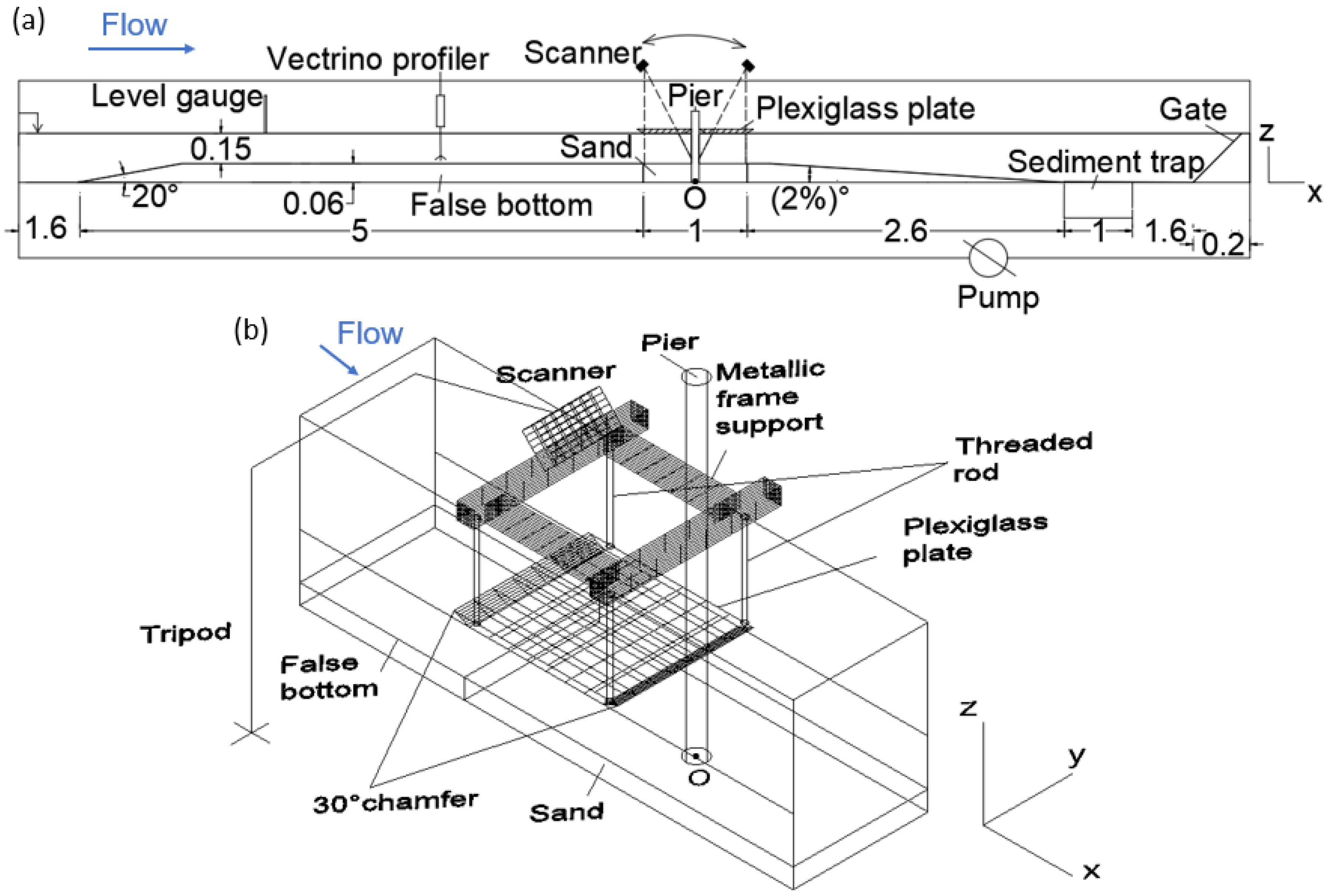
2. Flume Setup and Implementation of 3D Scanner Technique

The experiments were conducted in a rectangular flume that was 13 m long, 0.41 m wide and 0.5 m deep. The experimental setup of the pier scour model implemented in the flume is presented in Figure 1. A recess area that was 1 m long and 0.06 m deep was installed at a distance of 6.6 m beyond the flume entrance (Figure 1a). In order to contain the soil, a false bottom floor made of poly vinyl chloride (PVC), matching the depth of the recess area, was placed along the flume. The pier was modelled using a filled PVC cylinder with a diameter (b) of 0.032 m and a length of 1 m. As suggested by Whitehouse [31], the ratio between the pier diameter and the flume width was below 1/6 to avoid flow constriction. The reference system origin is located at the center of the circular pier. The x-axis denotes the longitudinal axis within the flume, oriented positively in the direction of flow. The z-axis represents the bed elevation, with positive values pointing upward. The y-axis indicates the transverse direction, with its positive orientation identified within the orthonormal reference system. A manual level gauge was used to measure the flow depth with an accuracy of ±0.5 mm. The flow depth measurement was made at the x-coordinate −2 m. The flow depth (h) was consistently fixed at 0.15 m throughout all tests. A Nortek Vectrino Profiler (Nortek AS, Vangkroken 2, 1351 Rud, Norway) was used to measure the velocity profile with a manufacturer accuracy of ±0.5% of the recorded value ±1 m/s [32]. The velocity measurement was carried out at the x-coordinate −0.7 m.

The evolution of the bed in the vicinity of the pier was continuously monitored using a Photoneo Scanner, type PhoXi 3D Scanner size S. It comprises a camera and a laser class 3R pattern projector. The scanner’s properties are summarized in

Table 1. Summary of Photoneo PhoXi 3D Scanner size S parameters.

Parameter	Value
Signal wavelength	around 639 nm in the red spectrum
Resolution	Up to 3.2 million points
Scanning volume shape	Trapezoidal
Scanning range	384–520 mm
Optimum scanning distance	442 mm
Scanning area at optimum distance	360 × 286 mm
Scanning time	250–2250 ms
Cost	around 20,000 €

.

The measuring concept is based on a sophisticated 3D surface imaging technology using structured light. This concept was described by Gupta and Nakhate [33] as follows: Multiple light planes emitted by the projector encompass the entire scene in the form of patterns. The surface geometry distorts these structural light patterns, assigning a unique intensity code to each projection column. By employing various structural light principles and algorithms, a correspondence between this intensity and the camera pixel is established. The 3D dimensional coordinates are then computed for the corresponding point on the scene using the triangulation plane theory, with knowledge of the distance between the laser source and the camera (230 mm), which allows for the automatic construction of the 3D object shape.

Initially, the scanner was oriented towards the glass wall of the flume. However, it was observed that this orientation prevented the measurement of the scour hole, resulting in a blind area. This issue likely arose due to the slight inclination of the incident pattern relative to the normal at the glass wall. The scanner was reoriented towards the water surface. To obtain full scour hole data around the pier, two experiments were conducted in the same conditions using the single available scanner, positioned either upstream or downstream of the pier. The scanner facilitated acquiring a half-plane view of the scour hole in each test. Surface waves near the pier caused the laser beams emitted by the scanner to diffract, resulting in unreliable measurements. To resolve this, a plexiglass plate was placed on the water surface throughout the measurements (Figure 1b). This plate, measuring 0.01 m in thickness and 0.5 m in length, spanned the entire width of the flume. It was firmly attached by threaded rods to a metal frame support positioned along the banks of the flume. As a result, the plate could not respond to water level changes, leading a pressure condition beneath it. The plate has ${30}^{\circ }$ chamfer at each end to direct flow and guarantee a flat water surface underneath.

3. Experimental Conditions

3.1. Sand Properties

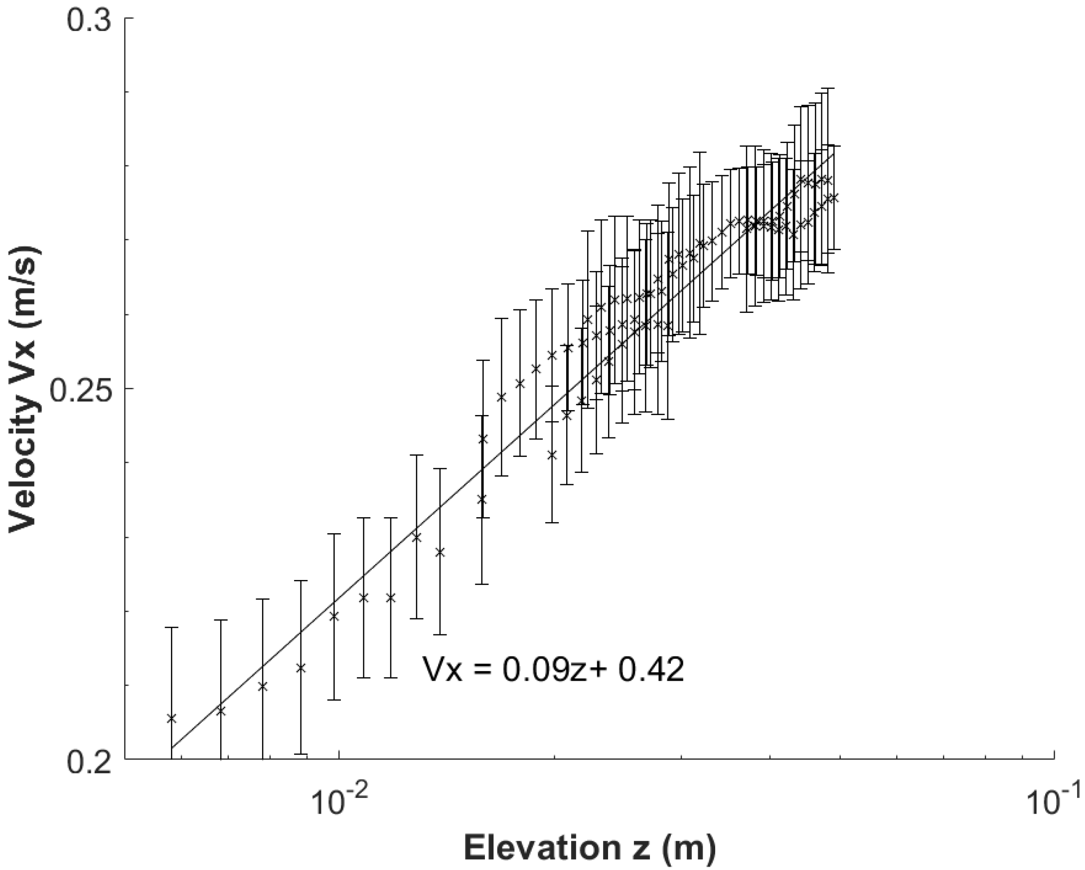
In this study, quartz-based sediment Hostun sand HN 1/2.5 was used. Figure 2 shows its particle size distribution curve.

Table 2. Experimental setup parameters; In sediment properties, $d_i$ represents sieve size for which i% of weighted soil is finer; in Reynolds number expressions, $\nu$ is the fluid kinematic viscosity (m²/s); in the Froude number expression, g is the acceleration of gravity (m²/s).

Sediment Properties		Flow Condition
medium diameter $d_{50}$ (μm)	1700	Depth-averaged flow rate Q (m3/h)	65
Geometric standard deviation ${\sigma }_g^2$ = ${\displaystyle \frac{d_{84}}{d_{16}}}$	1.2	Water depth h (m)	0.15
Uniformity coefficient $C_u={\displaystyle \frac{d_{60}}{d_{10}}}$	1.4	Depth-averaged current velocity V (m/s)	0.29
Coefficient of curvature $C_c={\displaystyle \frac{{\left(d_{30}\right)}^2}{d_{60}\times d_{10}}}$	1	Reynolds number based on the water depth $Re={\displaystyle \frac{V\times h}{\nu }}$	43,500
Internal friction angle $\varphi$ (°)	35	Reynolds number based on the pier diameter $R{e}_b={\displaystyle \frac{V\times b}{\nu }}$	9280
Cohesion C (kPa)	0	Froude number $Fr={\displaystyle \frac{V}{\sqrt{g\times h}}}$	0.24
Initial moisture content (%)	4	Flow intensity ${\displaystyle \frac{V}{Vcr}}$	0.7
Dry weight density (t/m3)	1.7

presents the values for the median diameter ($d_{50}$), geometric standard deviation (${\sigma }_g^2$), uniformity coefficient ($C_u$), coefficient of curvature ($C_c$), internal friction angle ($\varphi$), and cohesion (C) of the tested sand.

According to Wentworth [34], the sand falls under the very coarse grain size classification (1000 μm < $d_{50}$ < 2000 μm). According to the Soulsby [35] criterion, this sand is well sorted (${\sigma }_g^2$ < 2). The sand is uniformly graded, based on the values of $C_u$ and $C_c$. The sand has a relative density $s={\displaystyle \frac{{\rho }_s}{\rho }}=2.65$, where ${\rho }_s$ and $\rho$ are the densities of the sand and the fluid, respectively. Direct shear test measurements reveal the shear strength data, $\varphi$ and C, of the used sand.

The sand bed was prepared and then placed in the test section. The values of initial moisture and dry weight density are provided in Table 2. Once the sand was in place, the flume was filled with water very gently to avoid undesirable initial erosion. In order to achieve geotechnical conditions that are similar to those in the field, the soil was saturated for 1 h.

Initially, experiments were conducted without a pier in the flume. A low depth averaged current velocity (0.1 m/s) was set at the beginning of the experiment. Following the methodology of Lachaussée et al. [20], the threshold velocity was visually determined by gradually increasing the depth averaged current velocity in increments of 8 mm/s until at least three grains were observed to move within approximately 1 min. To confirm the obtained threshold value, a slight increase in depth averaged current velocity above the threshold should result in significant grain mobilization. The non-pier flume test was repeated three times, resulting in an average critical velocity $V_{cr}$ = 0.41 m/s (±0.005 m/s).

3.2. Flow Condition

The Vectrino Profiler was set to its highest measurement frequencies: 100 Hz for velocity and 10 Hz for bottom elevation, with an optimal spatial resolution of 1 mm. It was configured to measure velocity data within its maximum vertical range of 30 mm. Each velocity profile within this range represents the average of several instantaneous measurements recorded over 1 min. To obtain a vertical profile of the velocity over a greater elevation, the instrument was lowered approximately 15 mm towards the bottom, resulting in a 50% overlap. In our measurement, these data points were gathered from measurements performed at five different elevations above the smooth false floor. The sensor displacement uncertainty (±0.1 mm) caused a difference in elevation between the measurement elevations in the overlap area. We applied a filtering procedure to exclude velocity measurements that had the following: beam correlation below 80%, signal to noise ratio (SNR) below 20 dB, and a standard deviation exceeding 20% of the measured velocity value. Figure 3 displays the horizontal component of flow velocity ($V_x$) as function of the elevation (z) on a semi-logarithmic scale. The velocity distribution can be expressed in the logarithmic layer as follows [36]:

$${\displaystyle \frac{V_x\left(z\right)}{u_{*}}}={\displaystyle \frac{1}{K}}ln\left({\displaystyle \frac{z}{z_0}}\right)$$

(1)

where, $u_{*}$ (m/s) is the bottom friction velocity, K = 0.4 is the von Karman, constant and $z_0$ (m) is a length scale.

The measured velocity profile fits the logarithmic law approximately for 0.005 m < z < 0.05 m. The value of $u_{*}$ was derived from the slope of this linear relationship, given by ${\displaystyle \frac{u_{*}}{K}}$. Furthermore, $z_0$ is identified as null velocity elevation, the elevation of the point where the log-layer intersects the z-axis. The obtained values of $u_{*}$ and $z_0$ are 0.036 m/s and $0.21\times {10}^{-4}$ m, respectively.

Table 2 above shows the values of the depth-averaged flow rate (Q), the depth-averaged current velocity (V), the Reynolds number based on the water depth h ($Re$), the Reynolds number based on the cylinder diameter b ($R{e}_b$), the Froude number (Fr), and the flow intensity (${\displaystyle \frac{V}{Vcr}}$). The Q measurement collected using a flow meter, was used to predict the value of V. The velocity remained constant throughout the experiment. Based on this constant velocity, the dimensionless parameters for the flume tests were computed. The $Re$ denotes that the flow regime of the experiments is turbulent [36]. Laminar boundary layer separation with a fully turbulent wake zone is indicated by the $R{e}_b$ [37]. The subcritical hydraulic condition is indicated by the Fr. The flow intensity reveals a clear water scour regime.

4. Framework for Data Treatment

A framework for the treatment of data acquired by this scanner was developed. Figure 4 illustrates the successive steps of this strategy. In the following, detailed information on each step will be provided.

4.1. Data Acquisition

For acquiring 3D scans around the pier, the scanner was interfaced with PhoXi Control software. In our measurements, appropriate acquisition parameters were selected. Choosing a laser power of 4095 μWatt and an exposure time of 20.48 ms effectively prevented overexposure and camera saturation in our measurements. Measurements can be performed without the need for safety glasses. The parameters for shutter multiply, indicating the number of repetitions of a pattern (set to 1), and scan multiply, representing the number of repetitions of a scan (also set to 1), resulted in a high density of original cloud data, containing up to 1.3 million 3D points. An acquisition method with minimal interference from ambient light was also chosen. Hence, no dark experimental setup was required. Scans were automatically triggered at a fixed frame rate and were then automatically saved in “.ply” format. The frequency rate of acquisition was adjusted at 0.5 Hz for the first 5 min (1 scan per 2 s) due to the rapid scour process in sand at the beginning of the tests. It was then set to 0.0033 Hz (1 scan per 5 min) for the rest of the experiment. Several scans were then selected, which were sufficient for the study of the local scour phenomenon around the pier.

4.2. Calibration

Calibration was required for each of the two scanner positions. The operator must ensure that the device is well fixed without any movement, such as vibration, during the test run. This calibration will result in corrections that will be applied to all the data clouds acquired by the scanner.

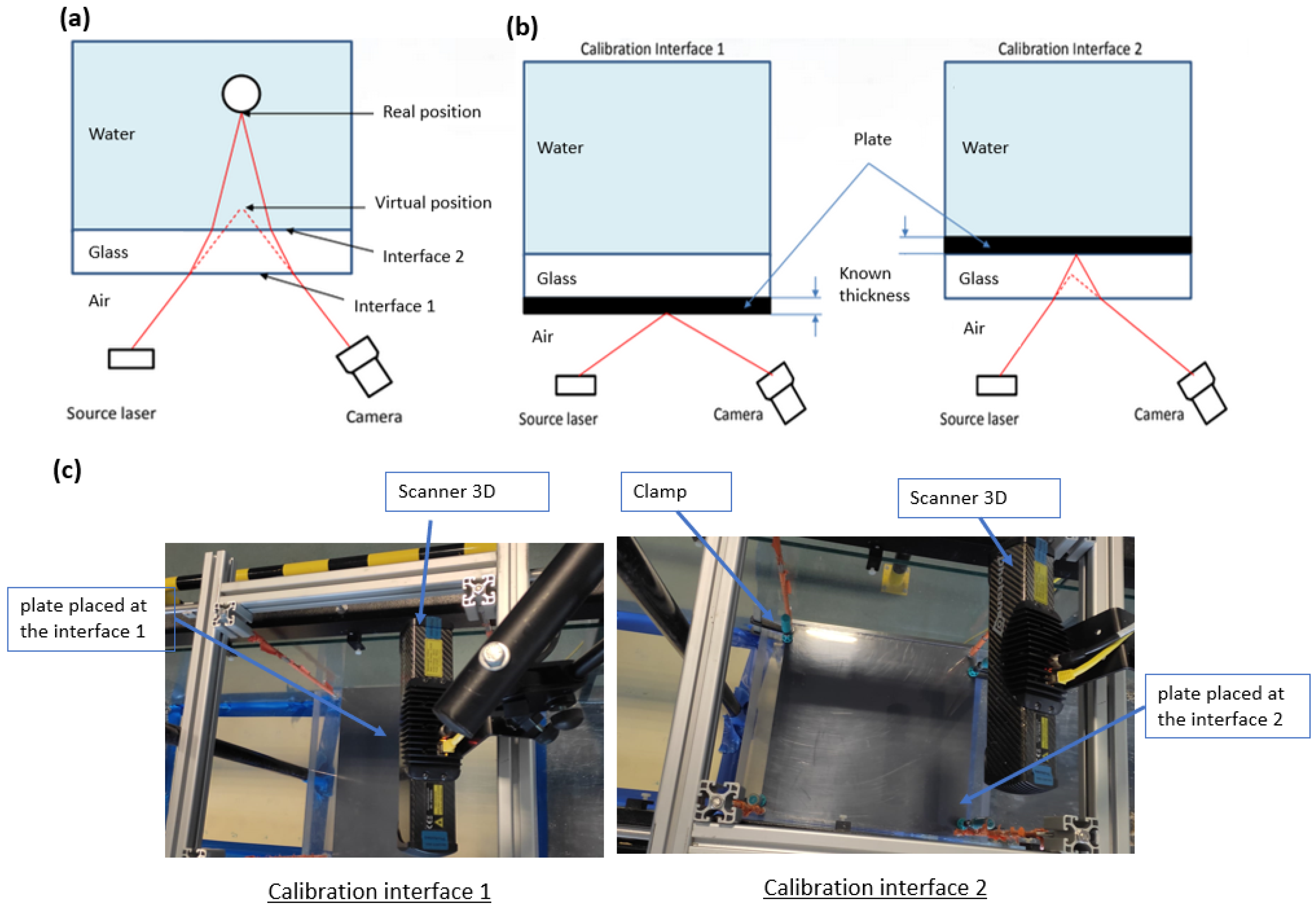
4.2.1. Refraction Correction

When a light ray passes through the interface between two distinct materials, its trajectory is changed due to refraction (Figure 5a). To take account of the refraction of the light, a correction algorithm developed by R&D Vision was used with the Scilab software. Applying this correction algorithm required determining the positions of interface 1 (between air and glass) and interface 2 (between glass and water) based on the positions of the camera and the laser device. A reference plate—an object of known thickness—should be scanned at each of the two interfaces, which will allow us to know these positions (Figure 5b,c). Clamps were used to fix the plate at the interface 2. To prevent the formation of air bubbles, this step was carried out in an empty flume before each test. The point clouds from both interfaces were in the “.ply” format. After acquiring all the data for the scour hole topography (also in “.ply” format), the Scilab code was executed. This script was employed to read the ply files and perform ray tracing calculations using matrix functions. It allowed for the correction of each acquired scan, resulting in a corresponding corrected scan in “.ply” format.

To demonstrate the need for this correction step, an application was performed using the 32 mm diameter cylinder used in the physical model. It was scanned white in color (before being painted black). The scanner was positioned in the upstream part focusing on the cylinder at a water depth of 15 cm. Figure 6a shows the scanned cylinder in air and in the presence of water and plexiglass before and after refraction correction visualized using Cloudcompare software. The surface of the cylinder scanned in the presence of water and plexiglass before correction was observed not to be at all a circle. This observation suggests that refraction has the potential to significantly modify the shape of the scanned object. The refraction correction resulted in a nearly cylindrical shape, although its relative spatial position was not precisely the same. The refraction correction applied to the underwater scene allows us to restore the accurate geometry without distortion, but it does not place the elements in their exact correct spatial position relative to reality.

The data sheet for the Photoneo Scanner specifies a spatial error margin of 0.05 mm [38]. This error is for a scanned object located in the air. The R&D Vision supplier of the 3D scanner instrumentation states that directly evaluating the measurement error of Photoneo for an object submerged in water is challenging due to non-linear deformations caused by refraction. Even after running the code correction in Scilab, it is not possible to achieve perfect correction. Therefore, to assess Photoneo error in a water medium, it is essential to calculate the relative deformation of the object after correction in comparison to the object scanned without water. From the measurements presented for the cylinder case, this error was quantified as follows. The “fine registration” tool embedded in CloudCompare software [39] was first used. It operates automatically based on the Iterative Closest Point (ICP) algorithm. Originally proposed by Besl and McKay [40], the ICP algorithm registers a “data” point cloud (H) to achieve the best alignment with a “model” point cloud (G) [40]. In our case, cloud H corresponds to the red cloud in the water medium after correction, and cloud G corresponds to the green cloud in the air medium (Figure 6a). Although the corresponding points in both clouds are close, they are not perfectly aligned, so we assume the clouds are already roughly registered. The procedure of ICP involves the following key steps [41,42]: (i) finding nearest neighbor matching based on the minimum Euclidean distance, (ii) computing transformation parameters (rotation and translation matrices), (iii) transforming the point cloud (H), and (iv) providing the optimum alignment as the result of an iterative process. Iterations continue until the “root mean square (RMS) difference” reaches a predefined threshold or until a set “number of iterations” is completed. For this analysis, we used a threshold of ${10}^{-7}$ for the RMS to ensure a precise alignment, being the lowest possible value in CloudCompare. Once the point clouds are spatially registered, the CloudCompare’s tool “C2C (Cloud to Cloud) absolute distance” was performed. The C2C is based on finding the Euclidean distance between the “nearest neighbour point” in the reference cloud (green cloud in the air medium (Figure 6a)) to each point in the second cloud (red cloud in the water medium after correction (Figure 6a)) [43]. The distribution of the C2C absolute distance along the submerged length of the cylinder is shown in Figure 6b. The highest difference was observed on the edges because in this region, the density of the cloud is the lowest. The average of the error distribution obtained in the static water condition was equal to 0.11 mm. It is important to note that the 0.11 mm does not correspond directly to the residual refraction error. It was considered the mean error that corresponds to Photoneo Sensor error in water and after applying the correction code. The observed value is within the range of the measurement uncertainty given by the Photoneo manufacturer, 0.1–0.2 mm. The 0.2 mm given by the Photoneo manufacturer corresponds to scanner positions too far from the scene being scanned, which was not the case in our study.

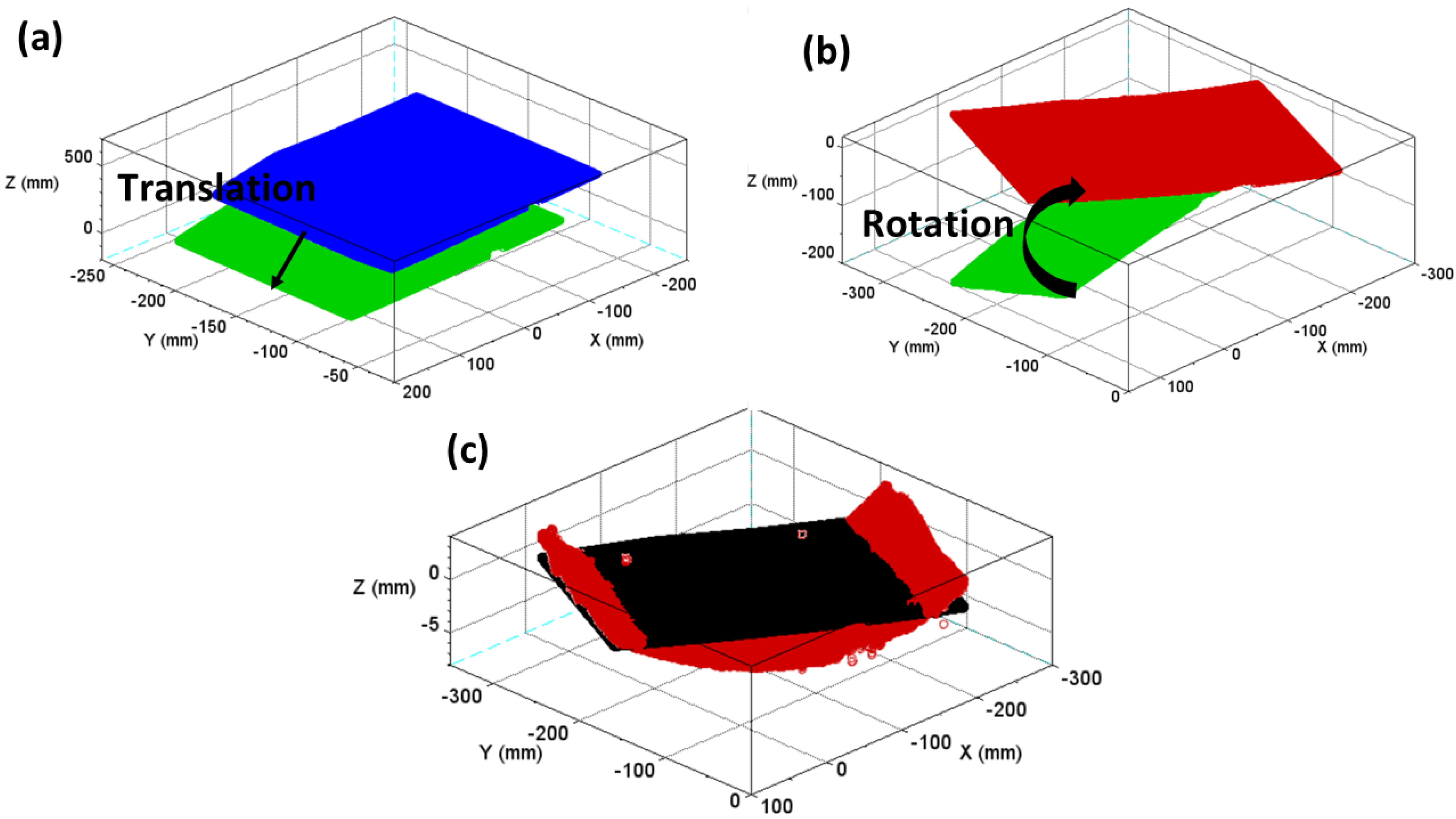
4.2.2. Reference Change

The (xyz) coordinates were used to identify the location of each point in a point cloud. The coordinate system (x′y′z′) in the scanner is located at the center projection pinhole of the camera. The camera sensor is inclined at 15.45° with respect to the sensor’s body [44]. In the camera space reference, the x′-axis points to the device’s right side and the y′-axis points below the device [44]. The depth at which the object was observed by the scanner was determined by the z′-axis [44]. The z′-axis aims to the scene perpendicular to the (x′y′) camera plane [44]. The device offers the capability to convert the point cloud into any user-defined coordinate space. However, the refraction code was developed in the camera space coordinate system. For this reason, it was required that the acquisition by the scanner was performed using the camera’s reference, subsequently applying the necessary of light refraction correction, and finally the step of the reference change.

An algorithm was integrated into the existing Scilab code for refraction correction, allowing the transformation of camera space coordinates (x′y′z′) to a local coordinate system (xyz) centered on the pier. This process involves determining the rotation and translation matrices and applying them to all points in the point cloud.

The outcomes of a practical application example within a smooth PVC flat plate configuration are illustrated in Figure 7. Despite scanning a flat plate, the resulting point cloud does not form a perfect plane. Variations from the mean plane were observed in the point cloud, reflecting the uncertainty in the measurement of the 3D scanner. The maximum deviation was observed at the edges of the acquisition zone. The presence of this slight curvature is probably due to the sphericity of the fisheye lenses.

4.3. Post-Treatment

The post-treatment step, including cloud cleaning and relative rasterization, was performed using CloudCompare. This software was selected for its compatibility with “.ply” file formats, its open-source nature, and its extensive use in the post-processing of scanner-acquired point clouds by many authors, e.g., Lague et al. [43], Rajendra et al. [45], Yang [46].

4.3.1. Cloud Cleaning

Scanner data invariably include scatter points and noise, impeding accurate identification of object details. Scatter points are those not belonging to the bed surface. Noise is caused by the laser beam’s divergence. The pier in our physical model was colored black, allowing for the removal of all its points. The CloudCompare software was used to manually clean the scanned clouds by eliminating all scatter points and minimizing noise as much as possible.

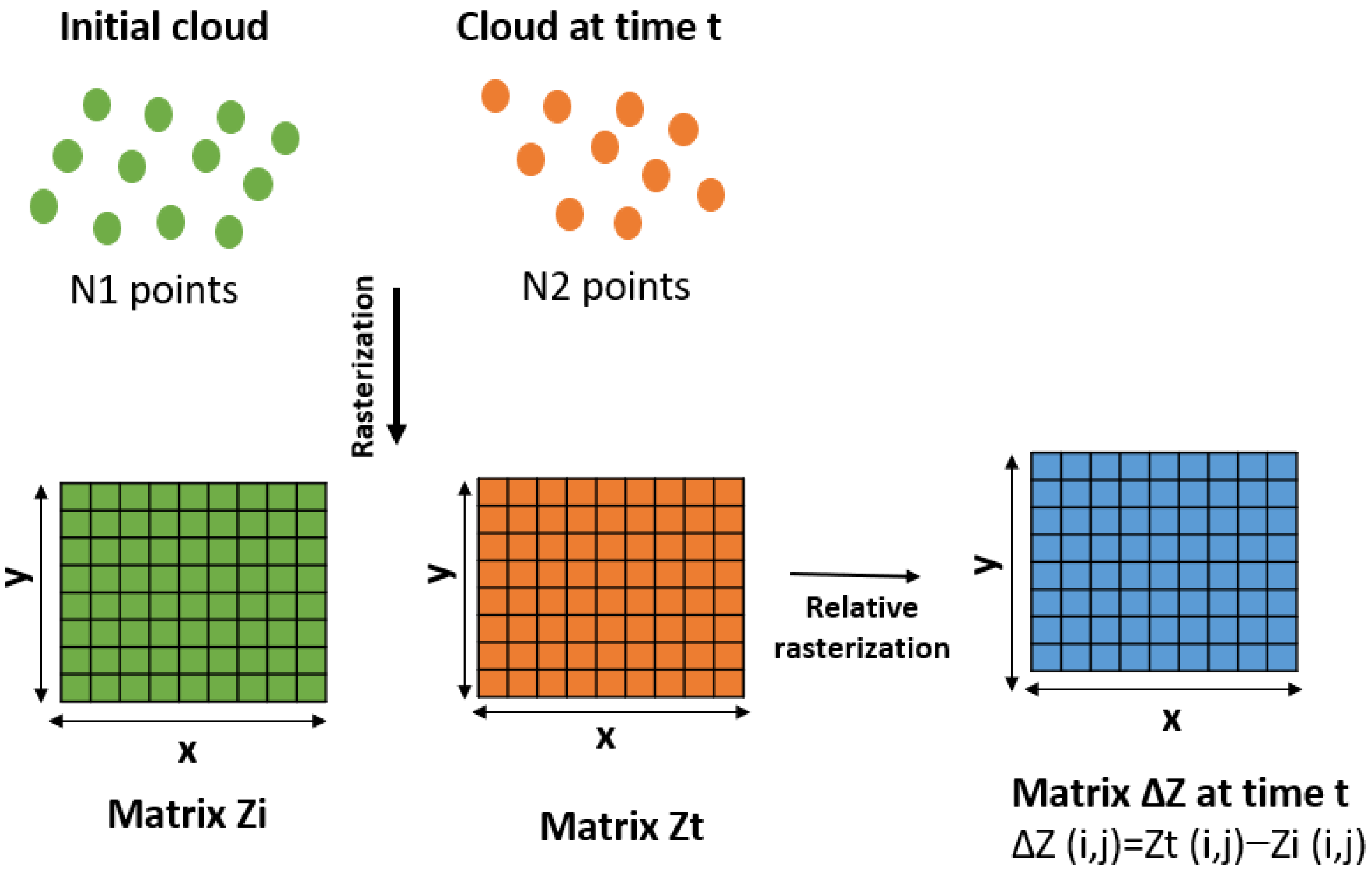
4.3.2. Relative Rasterization

A relative rasterization with the reference cloud, which is always the initial state of the soil (flat bed surface), was adapted. Figure 8 provides a visual representation to enhance the understanding of this step. This step was performed due to several reasons:

• The number of points among the different clouds exhibits variations.
• The point density within a single scan is non-uniform, decreasing as the distance from the scanner increases.
• The scan of a flat plate reveals a vertical deviation from a perfectly flat plane.

Each 3D cloud was converted into an elevation Z matrix, saved in “.txt” format, where lines and columns represented x and y coordinates, respectively. At each time interval t, the relative elevation data in matrix $\Delta Z$ represents the difference between the matrix Zt at time t and the matrix Zi at the initial time (Figure 8). This conversion was performed manually for every cloud using CloudCompare’s “Relative rasterization” tool. The parameters of this tool—center, dimensions (width, length), and grid size—remained consistent for each cloud in every specific test. A fixed horizontal grid resolution of 1 × 1 mm was chosen for our digital elevation model.

4.4. Representation

Once the Z matrices were well defined, MATLAB software [47] was used to represent the data. To enhance result quality and achieve a precise digital elevation model, a code for linear interpolation was written in MATLAB to replace missing data points by numbers obtained by linear interpolation between two neighboring points. The results were presented using MATLAB software in different representation forms (counter map plot, scour depth function of azimuth angle, section profiles, etc.) as shown in Section 5.

5. Results

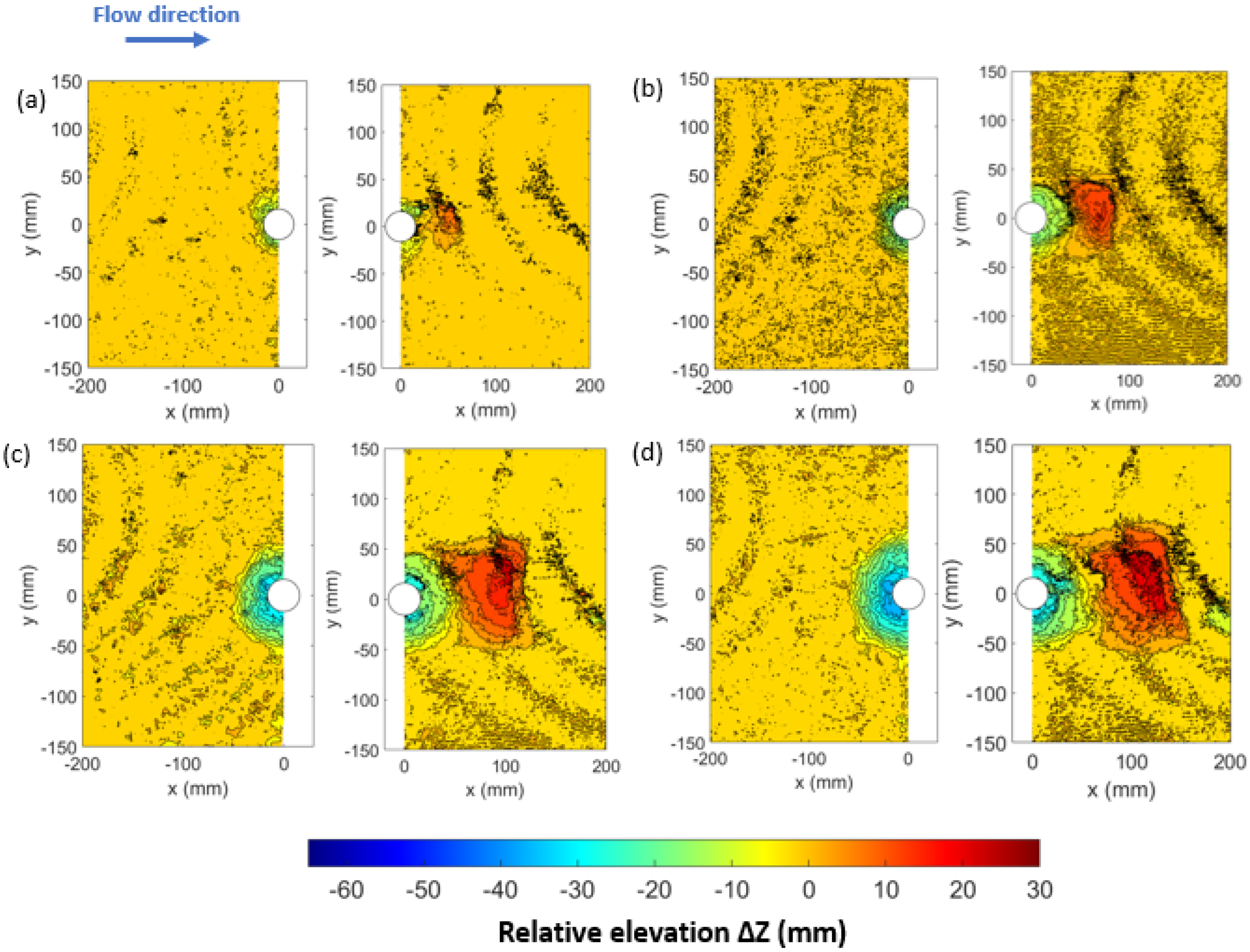
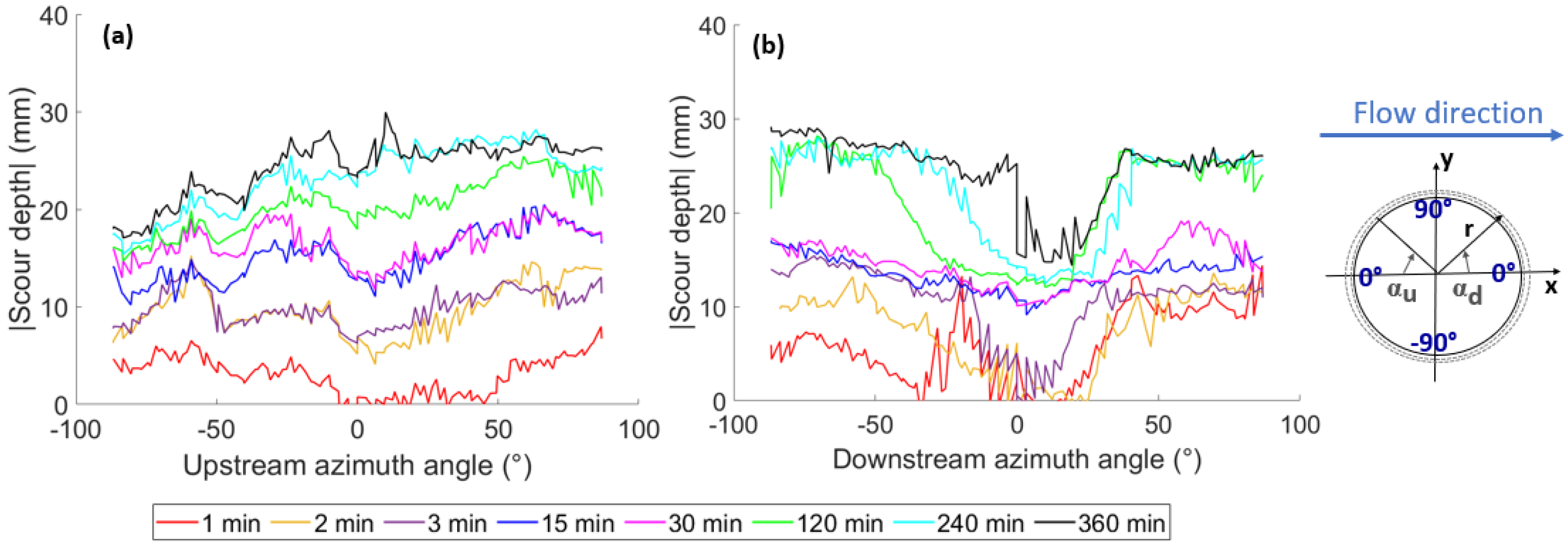
5.1. Spatio-Temporal Progression of the Scouring Phenomenon

Figure 9 shows the contour maps of the relative elevation $\Delta Z$ from data collected during both upstream and downstream tests at different time intervals, including 2 min, 15 min, 120 min, and 360 min. The observed local scour pattern was characterized by a scour hole around the pier and a single dune. This finding was consistent with the classical scour hole pattern observed on a cohesionless bed in clear water scour regime in the literature [12,48]. During the scour process, the general shape of the scour hole remained almost the same and nearly symmetrical relative to the flow direction. The artefact in the contour map was due to a light spot inadvertently placed near the test section during the measurements.

The presence of the pier caused a contraction of the flow, resulting in an acceleration that swept and ejected the eroded sediments from the scour hole downstream. The sediments were deposited downstream of the pier, gradually forming a dune. Over time, the dune gradually increased in height. Eventually, it reached a maximum value close to 0.8 times the diameter of the pier within a measurement period of 360 min. Since the scour process was in progress, the sediments in the dune continued to accumulate, being carried by wake vortices far downstream until reaching an equilibrium state.

Figure 10 illustrates the scour depth as a function of the azimuth angles for the upstream part (${\alpha }_u$) and the downstream part (${\alpha }_d$) of the pier at various instants (1 min, 2 min, 3 min, 15 min, 30 min, 120 min and 360 min). The region of interest includes all points with radial coordinates (r) from 17 to 19 mm, positioned 1 to 3 mm away from the cylinder’s outer surface. The upstream azimuth angle (${\alpha }_u$) was measured clockwise from the horizontal axis opposite to the flow direction. Conversely, the downstream azimuth angle (${\alpha }_d$) was measured counterclockwise from the horizontal axis in the direction of the flow. At 1 min, depressions formed at the sides of the pier, marking the initiation of the scour process (Figure 10a). The scour depths at 2 min and 3 min were larger on the sides than the front of the pier (Figure 9a and Figure 10a). This is in accordance with the initial shear stress distribution around a pier reported in the literature [21,49]. After 15 min, the scoured region enlarged to cover the entire area surrounding the pier (Figure 9b and Figure 10a). At this stage, the scour depths were nearly equal around the pier. Subsequently, the scour hole progressively widened and deepened, with the maximum final scour depth at the front of the pier exceeding that at the side region by the end of the experiment (Figure 9d and Figure 10a). On the other hand, the scour depths at the downstream center region consistently remained the smallest (Figure 9 and Figure 10b).

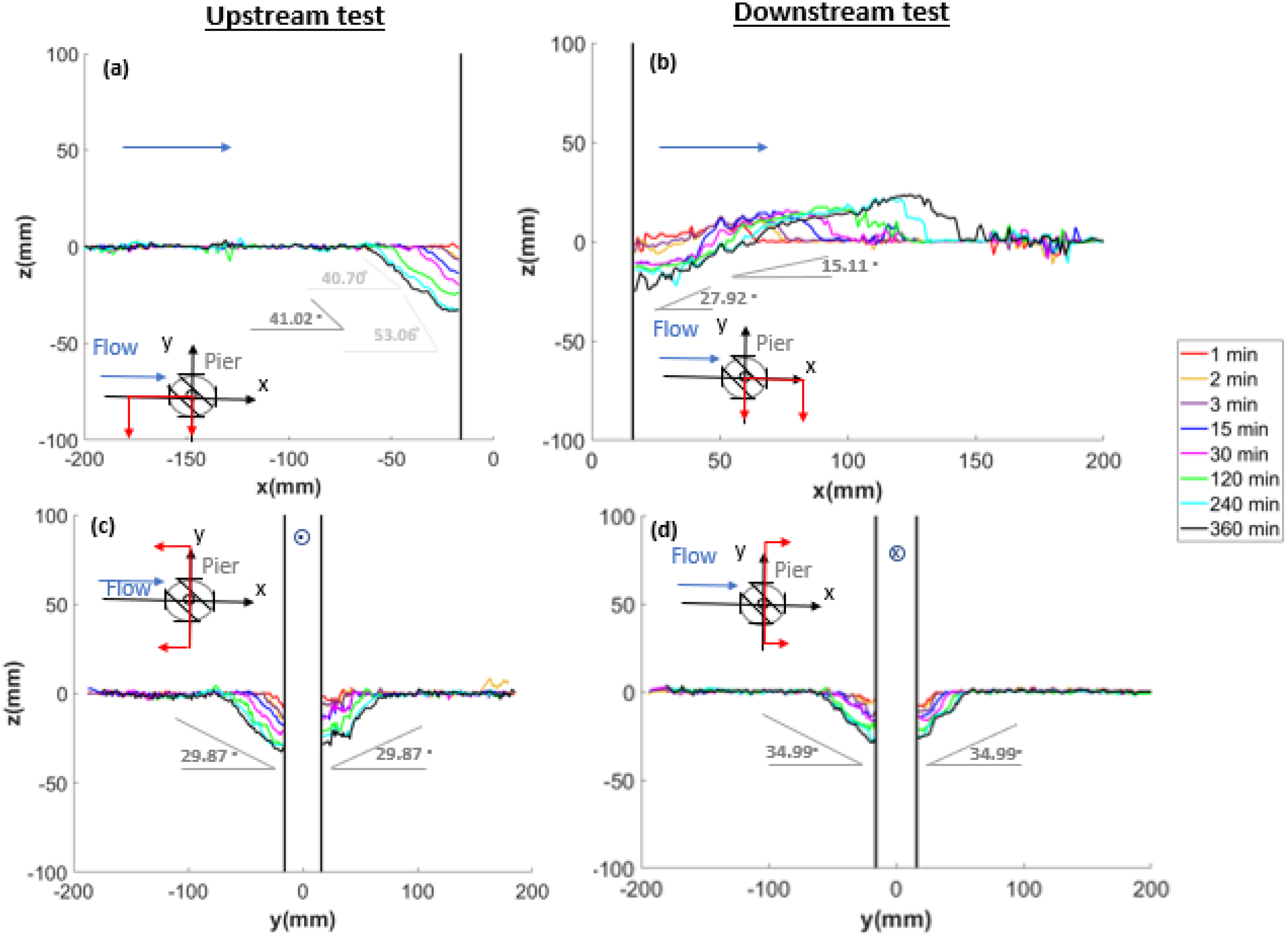
5.2. Temporal Evolution of the Scour Hole Profiles

Figure 11 represents the temporal variation of the scour profiles at the longitudinal centerlines (y = 0) and the transverse centerlines (x = 0).

In longitudinal and transversal sections, the existence of a flat bottom region close to the pier was identified quantitatively using the scanner 3D and visually. Obtaining topographical measurements in this area was hindered by the presence of the pier, which posed limitations across various instrumentation methods. This constraint was noted in studies, by Lachaussée et al. [20] utilizing profilometer laser technique, by Porter et al. [6] employing photogrammetry, and using a laser distance sensor by Link et al. [9].

The slope of the best fit straight line for each scour hole profile without the flattened portions was determined. The values of these slopes are almost constant during the part of the test from 15 min to 360 min. For the longitudinal profile at the upstream part, two slopes were recognized from the 15 min data record (Figure 11a). The ${\beta }_{lu1}$ represents the slope of the upstream section nearest to the pier, ${\beta }_{lu2}$ represents the slope of the upstream section farther from the pier, and ${\beta }_{lu}$ denotes the slope of the entire upstream section. The presence of two slopes in the upstream of the pier suggested the action of the horseshoe vortex system as reported by Dargahi [50]. This system is primarily responsible for bed deformation during scour in a cohesionless bed. The values obtained at the end of the experiment (360 min) for longitudinal slope at the upstream part are as follows: ${\beta }_{lu1}$ = $53.{06}^{\circ }$, ${\beta }_{lu2}$ = $40.{70}^{\circ }$, and ${\beta }_{lu}$ = $41.{02}^{\circ }$. The natural angle of repose of the sand HN 1/2.5 can be considered to be around the friction angle measured by the direct shear test, which is 35°. The observed scour slopes at the upstream part exceeds the natural angle of repose of sediment particles, which was consistent with the prior findings in various studies [51,52]. According to Dey [51], the average scour hole slope in this region is about 10–15% sharper than the natural angle of repose of sediment particles. The obtained average slope ${\beta }_{lu}=40.{02}^{\circ }$ at the end of the experiment was around 15% sharper than the natural angle of repose of sand HN1/2.5 particles. If measurements are taken after water pause or drainage, sediment will settle due to gravity. Consequently, the slope in this area will correspond to the natural angle of repose of the soil, as found by [5,53].

Therefore, at the end of the experiment, the longitudinal downstream part exhibited a slope (${\beta }_{ld1}$) of around 27.92°, with a slope (${\beta }_{ld2}$) of 15.11° observed at the dune (Figure 11b). The observed value of ${\beta }_{ld1}$ was consistent with the observation of Harris and Whitehouse [54], being around half of the angle of repose of the sediment +2°. Sediments moved downwards on the scour hole’s lower slope and upward on the dune’s upper slope. Wake vortices carried the downward-moving sediments as bed load to the upper slope. Sediments either passed through the dune or were continuously fed and were deposited at the mount.

On the other hand, for the central transversal profiles, ${\beta }_{su}$ and ${\beta }_{sd}$ represent the side slopes at the end of the experiment from the upstream test and the downstream test, respectively. The slope value on the sides for each test is the average value of the slope on the left and right. The ${\beta }_{su}$ was measured at around 29.87° for the upstream test against ${\beta }_{sd}$ = 34.99° for the downstream test (Figure 11c,d). This corresponds to an average side slope value of 32.43°. This value was close to the natural angle of repose of the sand HN1/2.5 in agreement with the literature [55,56].

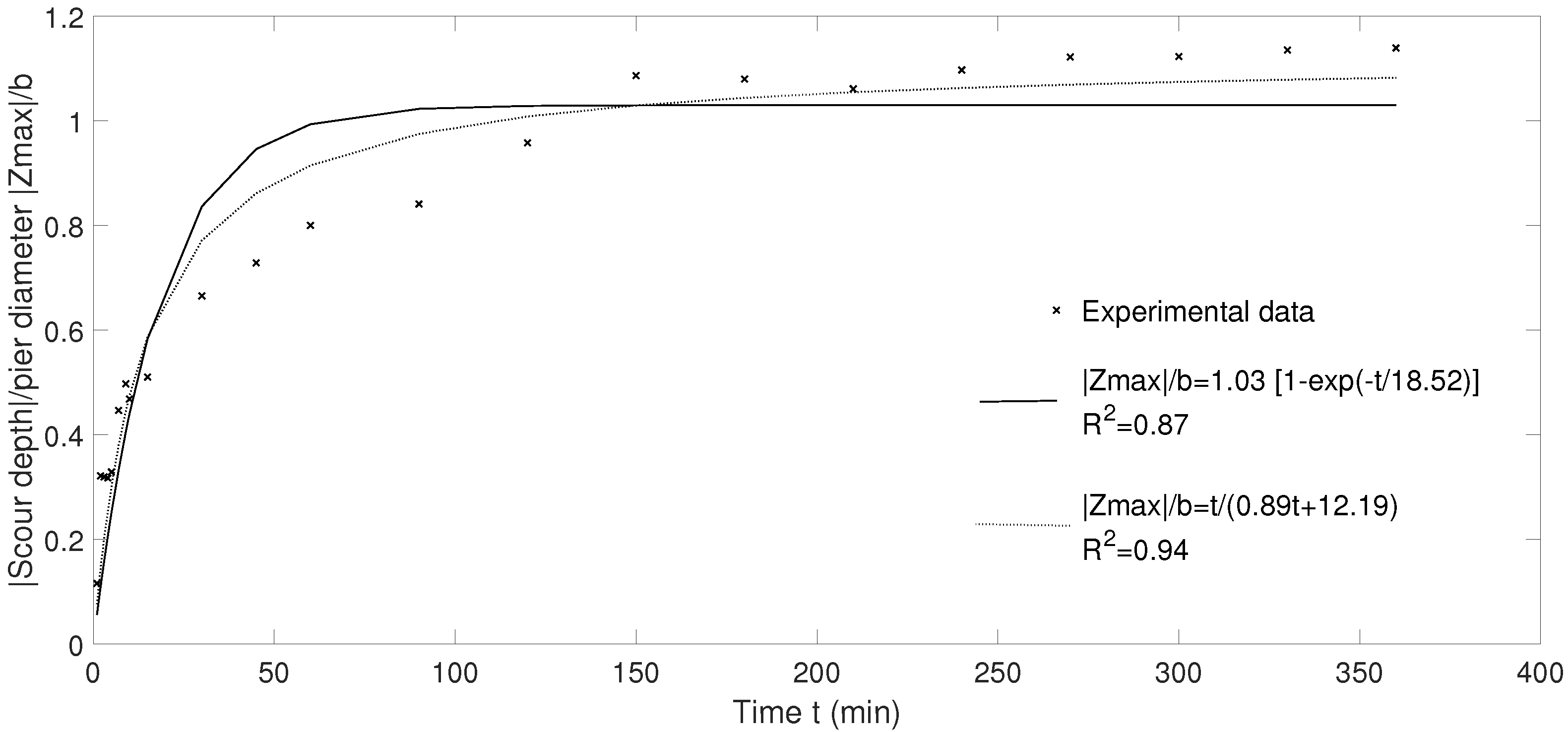
5.3. Temporal Variation of Maximum Scour Depth

The position of the maximum scour depth point was identified based on experimental measurements obtained at the end of the tests (at 360 min). This was performed for both upstream and downstream experiments. The point with the greatest depth value, from either tests, was selected. The coordinates of the point are as follows: a radial distance of r = 19 mm (at 3 mm from the pier face) and an upstream azimuth angle of ${\alpha }_u=7^{\circ }$ with respect to the pier. This was consistent with findings from earlier studies on a cohesionless bed in clear water scour regime [57,58,59].

Figure 12 presents the temporal evolution of the non-dimensional scour depth at the location where the final maximum scour depth was previously determined. During the early phase of the scour process, the scour depth increased rapidly, reaching over 60% of its final depth within the first 30 min. It increased then slower until an asymptotic final state was eventually reached at 240 min. The maximum final scour depth recorded was 1.1 times the pier’s diameter ($|Z_{\max }|$(360 min) = 1.1 × b). This was consistent with the reported values in the literature [21,58,60]. The best trend curves for the exponential and hyperbolic laws were determined from the measured data. These two laws were selected being commonly used in the literature [61,62,63,64] for the temporal evolution of the maximum scour depth. The regression coefficients obtained were of the order of 0.9, showing that these equations describe well the temporal evolution of the maximum scour depth.

5.4. Repeatability of the Tests

The experimental procedure raises the issue of test repeatability, since a full geometry of the scour hole will result from two experiments. The quantification of the error due to test repeatability was performed based on a total of six tests: three tests upstream of the pier and three tests downstream of the pier.

For each point P within the data set, the mean depth $Z_{p\left(average\right)}$ and the standard deviation ${\sigma }_p$ were calculated. The punctual mean depth $Z_{p\left(average\right)}$ was determined by averaging the depths $Z_{p\left(i\right)}$ from each of the three tests, denoted by the index (i) ranging from 1 to 3. The punctual standard deviation for each data point was computed using the formula ${\sigma }_P={\displaystyle \frac{\sum {\left(Z_{p\left(\mathrm{i}\right)}-Z_{p\left(\mathrm{average}\right)}\right)}^2}{n-1}}$, where n equals the number of tests, which is 3.

Figure 13 illustrates the spatial distribution of the $Z_{p\left(average\right)}$ and ${\sigma }_p$ across the measured zones at 15 min and 360 min. The figure on the left represents the results obtained when the scanner is focused on the upstream part, while the figures on the right represent the results when the scanner is focused on the downstream part for each respective time. The standard deviation ($\sigma$) was the average of all punctual standard deviations (${\sigma }_p$) for data points where $Z_{p\left(average\right)}$ exceeds 0.11 mm or falls below −0.11 mm. Repeatability was checked for different times (5, 10, 15, 30, 45, and 60 min, followed by every 30 min up to 360 min). The resulting value of $\sigma$ was found to be within the 0.5–1.12 mm range, which was considered acceptable. It is also noticed that repeatability is lower in areas with steep slopes.

5.5. Effect of Plexiglass Plate on Pier Scour Topography

Two tests were conducted without the plexiglass plate covering the water surface. In the first test, the scanner focused on the upstream part of the pier, while in the second test, it focused on the downstream part of the pier. For each test, initially, the plexiglass plate was placed on the water surface to enable calibration and capture an initial scan before any soil erosion occurred. Subsequently, the plexiglass plate was removed, and the test was running for a duration of 360 min. At the end of the 360-min test run, the plexiglass plate was carefully replaced on the water surface and the topography of the scour was scanned.

A comparison of the contour maps of the scour topography at the end of tests (360 min) for tests with and without the plexiglass plate is shown in Figure 14a,b. The figures on the left side refers to the results from the upstream tests and those on the right refers to results from the downstream tests. For tests with the plexiglass plate, the values taken are those of the average relative elevation $Z_{p\left(average\right)}$ from the three tests as previously described in the Section 5.4. The contours with and without the plate obtained were similar.

For a better view of the results, Figure 14c–f present a comparison of longitudinal and transversal profiles with and without the plexiglass plate. Figure 14c,e pertain to the results obtained from the upstream tests, while Figure 14d,f correspond to the results derived from the downstream tests. The red curve represents the punctual average scour depth $Z_{p\left(average\right)}$, which is the result of three tests. The corresponding error bar indicates the corresponding punctual standard deviation ${\sigma }_p$ as previously described in the Section 5.4. The longitudinal and transverse profiles without the plate lie within the error bar zone determined from repeatability tests with the plate.

These results confirm that under the tested hydraulic conditions, the plexiglass plate has a negligible effect on pier scour topography. The observed results contradicts the observations reported by [23,65] that the presence of a plate surrounding the bridge pier amplifies the pier scour. The Froude number in our study, on the order of 0.2, might be the reason for the negligible influence of the plate on pier scour as previously noted by Lachaussée et al. [20].

6. Discussion

In a non-cohesive soil benchmark tests, the results obtained with the scanner on local scour around a circular pier were close to those in the literature. This validates the proposed methodology and demonstrates its ability to dynamically measure the scour topography in a laboratory setting. It is important to note that this method was used in sand under a live bed scour regime and in mixed soils, non-cohesive and cohesive (with cohesive content ≤ 15%), and provided a good understanding of the scouring phenomenon [66]. In the following, we compare the instrument used in this study with the other imagery-based technique reported in the literature.

In comparing photogrammetry to the used scanner technique, several key differences emerge. The photogrammetry technique reported in Porter et al. [12] and Umeda et al. [6] required the flow to be stopped and the model to be drained during photo acquisition. This method can become quite laborious and time-consuming if the bed is measured at multiple instances. Additionally, this water interruption may cause disruptions that affect the erosion processes. Also, measuring the bed elevation intermittently assumes that the behavior of the bed during the intervening periods can be estimated through interpolation. However, this assumption may not always be accurate, as the rate of scour may vary over time and at different locations. Our technique can continuously capture real-time data without the need to stop the flow or drain the model, thus providing a continuous record of bed elevation changes over time. It is important to note that some studies using photogrammetry, such as Baglio et al. [13], did not account for lens distortions and light refraction through air, glass, and water interfaces. Although Summer et al. [15] did account for lens aberrations, they still did not replicate refraction through the flume wall properly. Our technique corrects for refraction, ensuring accurate measurements. Baglio et al. [13] made their measurements from a side view through a glass wall. However, using a side view may not be suitable for monitoring pier scour because the process might not be symmetrical. However, in our tests, measurements were taken from above, allowing a more comprehensive assessment. The data processing in photogrammetry, as proposed by Bouratsis et al. [14], is very lengthy due to the precise synchronization of video frames from two cameras, meticulous extraction of images, use of reference points for coordinate transformation, and the application of complex computer-vision and image-processing algorithms to accurately reconstruct the high-resolution 3D surface of the evolving sediment bed. In contrast, the data processing for the scanner method used in our study is much shorter and simpler.

The laser profilometer utilized in the study by Lachaussée et al. [20] generates 3D scour maps from each complete round trip, typically taking an average of 5 min. This method is noted as quasi-instantaneous with respect to the scour rate evolution. Their research focused exclusively on equilibrium states, maintaining a consistent placement of a plate on the water surface. In contrast, our scanner captures a cloud of all 3D points instantaneously with high temporal resolution. Our technique’s software automatically reconstructs 3D representations, whereas their data processing involves the more time-intensive task of grouping 2D profiles together.

7. Conclusions and Perspectives

The structured-light scanner demonstrates its capability to dynamically measure bed elevation changes during pier scour mechanisms in laboratory setups. A structured procedure is outlined for calibrating and processing acquired data to obtain 3D digital elevation data of shaped scour holes with high spatial accuracy. This approach represents a significant advancement in monitoring scour development around piers, offering rapid, automatic, and continuous monitoring without the need to drain or stop water flow. This method is described as non-intrusive under the hydraulic conditions of the tests conducted. The data processing is expedited compared to other methods due to the instrument’s automatic cloud reconstruction. However, limitations include the critical positioning required to avoid shadows from nearby objects and constraints on the acquisition zone dimensions. Factors such as turbidity and waves can also impact data acquisition quality, making this technique not applicable for real-world scenarios. Calibration is required before measurement for each scanner position, and any deviation of the instrument could lead to significant errors in the acquired data. The reflectivity of the surface being scanned can also affect the scanner’s ability to capture data, with absorptive surfaces leading to an absence of point cloud. Furthermore, the high cost of the used 3D scanner compared to other instrumentation and the need for specialized software can be a limitation of this technique. This study provides an experimental dataset for numerical simulations of very coarse granular sediment scour models.

Enhancements to the scanning acquisition include the integration of an additional scanner and extra plexiglass with synchronization measures on both upstream and downstream sides of the pier. It would be interesting to automate the step of rasterization and cleaning clouds. A comprehensive study involving turbidity levels variations is required to determine the onset of an effect. It is essential to conduct tests to determine if the plate used in our setup has an effect on pier scour for different experimental conditions than those considered in the present paper. It would also be interesting to explore the effect of installing a collar of specific thickness around the pier on the accuracy of 3D scanner measurements.

References

1. Melville, B.W.; Coleman, S.E. Bridge Scour; Water Resources Publication: Highlands Ranch, CO, USA, 2000. [Google Scholar]
2. Kirby, A.; Roca, M.; Kitchen, A.; Escarameia, M.; Chesterton, O. Manual on Scour at Bridges and Other Hydraulic Structures; Ciria: London, UK, 2015. [Google Scholar]
3. Oliveto, G.; Hager, W.H. Temporal evolution of clear-water pier and abutment scour. J. Hydraul. Eng. 2002, 128, 811–820. [Google Scholar] [CrossRef]
4. Lança, R.M.; Fael, C.S.; Maia, R.J.; Pêgo, J.P.; Cardoso, A.H. Clear-water scour at comparatively large cylindrical piers. J. Hydraul. Eng. 2013, 139, 1117–1125. [Google Scholar] [CrossRef]
5. Yanmaz, A.M.; Altinbilek, H.D. Study of time-depenbent local scour around bridge piers. J. Hydraul. Eng. 1991, 117, 1247–1268. [Google Scholar] [CrossRef]
6. Porter, K.; Simons, R.; Harris, J. Comparison of three techniques for scour depth measurement: Photogrammetry, echosounder profiling and a calibrated pile. In Proceedings of the 34th International Conference on Coastal Engineering (ICCE 2014), Seoul, Republic of Korea, 15–20 June 2014; p. 64. [Google Scholar]
7. Mia, M.F.; Nago, H. Design method of time-dependent local scour at circular bridge pier. J. Hydraul. Eng. 2003, 129, 420–427. [Google Scholar] [CrossRef]
8. Debnath, K.; Chaudhuri, S. Bridge pier scour in clay-sand mixed sediments at near-threshold velocity for sand. J. Hydraul. Eng. 2010, 136, 597–609. [Google Scholar] [CrossRef]
9. Link, O.; Gobert, C.; Manhart, M.; Zanke, U. Effect of the horseshoe vortex system on the geometry of a developing scour hole at a cylinder. In Proceedings of the 4th International Conference on Scour and Erosion (ICSE-4), Tokyo, Japan, 5–7 November 2008; pp. 162–168. [Google Scholar]
10. Ballio, F.; Radice, A. A non-touch sensor for local scour measurements. J. Hydraul. Res. 2003, 41, 105–108. [Google Scholar] [CrossRef]
11. Link, O.; Klischies, K.; Montalva, G.; Dey, S. Effects of bed compaction on scour at piers in sand-clay mixtures. J. Hydraul. Eng. 2013, 139, 1013–1019. [Google Scholar] [CrossRef]
12. Umeda, S.; Yamazaki, T.; Ishida, H. Time evolution of scour and deposition around a cylindrical pier in steady flow. In Proceedings of the 4th International Conference on Scour and Erosion (ICSE-4), Tokyo, Japan, 5–7 November 2008; pp. 140–146. [Google Scholar]
13. Baglio, S.; Faraci, C.; Foti, E.; Musumeci, R. Measurements of the 3-D scour process around a pile in an oscillating flow through a stereo vision approach. Measurement 2001, 30, 145–160. [Google Scholar] [CrossRef]
14. Bouratsis, P.; Diplas, P.; Dancey, C.L.; Apsilidis, N. High-resolution 3-D monitoring of evolving sediment beds. Water Resour. Res. 2013, 49, 977–992. [Google Scholar] [CrossRef]
15. Sumer, B.M.; Petersen, T.U.; Locatelli, L.; Fredsøe, J.; Musumeci, R.E.; Foti, E. Backfilling of a scour hole around a pile in waves and current. J. Waterw. Port Coastal Ocean. Eng. 2013, 139, 9–23. [Google Scholar] [CrossRef]
16. Bento, A.M.; Couto, L.; Viseu, T.; Pêgo, J.P. Image-based techniques for the advanced characterization of scour around bridge piers in laboratory. J. Hydraul. Eng. 2022, 148, 06022004. [Google Scholar] [CrossRef]
17. Foti, E.; Rabionet, I.C.; Marini, A.; Musumeci, R.E.; Sánchez-Arcilla, A. Experimental investigations of the bed evolution in wave flumes: Performance of 2D and 3D optical systems. Coast. Eng. 2011, 58, 606–622. [Google Scholar] [CrossRef]
18. Bouratsis, P.; Diplas, P.; Dancey, C.L.; Apsilidis, N. Quantitative spatio-temporal characterization of scour at the base of a cylinder. Water 2017, 9, 227. [Google Scholar] [CrossRef]
19. Poggi, D.; Kudryavtseva, N.O. Non-intrusive underwater measurement of local scour around a bridge pier. Water 2019, 11, 2063. [Google Scholar] [CrossRef]
20. Lachaussée, F.; Bertho, Y.; Morize, C.; Sauret, A.; Gondret, P. Competitive dynamics of two erosion patterns around a cylinder. Phys. Rev. Fluids 2018, 3, 012302. [Google Scholar] [CrossRef]
21. Roulund, A.; Sumer, B.M.; Fredsøe, J.; Michelsen, J. Numerical and experimental investigation of flow and scour around a circular pile. J. Fluid Mech. 2005, 534, 351–401. [Google Scholar] [CrossRef]
22. Ma, L.; Wang, L.; Guo, Z.; Jiang, H.; Gao, Y. Time development of scour around pile groups in tidal currents. Ocean. Eng. 2018, 163, 400–418. [Google Scholar] [CrossRef]
23. Sirianni, D.A.B.; Valela, C.; Rennie, C.D.; Nistor, I.; Almansour, H. Effects of developing ice covers on bridge pier scour. J. Hydraul. Res. 2022, 60, 645–655. [Google Scholar] [CrossRef]
24. Bestawy, A.; Eltahawy, T.; Alsaluli, A.; Almaliki, A.; Alqurashi, M. Reduction of local scour around a bridge pier by using different shapes of pier slots and collars. Water Supply 2020, 20, 1006–1015. [Google Scholar] [CrossRef]
25. Yagci, O.; Yildirim, I.; Celik, M.F.; Kitsikoudis, V.; Duran, Z.; Kirca, V.S.O. Clear water scour around a finite array of cylinders. Appl. Ocean. Res. 2017, 68, 114–129. [Google Scholar] [CrossRef]
26. Wu, M.; De Vos, L.; Chavez, C.E.A.; Stratigaki, V.; Whitehouse, R.; Baelus, L.; Troch, P. A study of scale effects in experiments of monopile scour protection stability. Coast. Eng. 2022, 178, 104217. [Google Scholar] [CrossRef]
27. Raju, R.D.; Nagarajan, S.; Arockiasamy, M.; Castillo, S. Feasibility of Using Green Laser in Monitoring Local Scour around Bridge Pier. Geomatics 2022, 2, 355–369. [Google Scholar] [CrossRef]
28. Lyu, X.; Cheng, Y.; Wang, W.; An, H.; Li, Y. Experimental study on local scour around submerged monopile under combined waves and current. Ocean. Eng. 2021, 240, 109929. [Google Scholar] [CrossRef]
29. Huang, K.; Wu, X.; Lin, Z. An advanced laboratorial measurement technique of scour topography based on the fusion method for 3D reconstruction. J. Ocean. Eng. Sci. 2023; in press. [Google Scholar] [CrossRef]
30. Zhou, K.; Duan, J.G.; Bombardelli, F. Experimental and theoretical study of local scour around three-pier group. J. Hydraul. Eng. 2020, 146, 04020069. [Google Scholar] [CrossRef]
31. Whitehouse, R. Scour at Marine Structures: A Manual for Practical Applications; Thomas Telford: London, UK, 1998. [Google Scholar]
32. NortekAs, Vectrino Profiler. Available online: http://www.nortek-as.com/en/products/velocimeters/vectrino-ii (accessed on 15 September 2020).
33. Gupta, M.; Nakhate, N. A geometric perspective on structured light coding. In Proceedings of the European Conference on Computer Vision (ECCV), Munich, Germany, 8–14 September 2018; pp. 87–102. [Google Scholar]
34. Wentworth, C.K. A scale of grade and class terms for clastic sediments. J. Geol. 1922, 30, 377–392. [Google Scholar] [CrossRef]
35. Soulsby, R.L. Dynamics of marine sands: A manual for practical applications. Oceanogr. Lit. Rev. 1997, 9, 947. [Google Scholar]
36. Sleath, J.F. Sea Bed Mechanics; Wiley: New York, NY, USA, 1984. [Google Scholar]
37. Sumer, B.M.; Fredsøe, J. Hydrodynamics around Cylindrical Structures; World Scientific: Singapore, 2006; Volume 26. [Google Scholar]
38. Photoneo, PhoXi 3D Scanner S Datasheet. Available online: https://www.photoneo.com/products/phoxi-scan-s/ (accessed on 20 November 2020).
39. Girardeau-Montaut, D. Détection de Changement sur des Données géométriques Tridimensionnelles. Doctoral Dissertation, Télécom ParisTech, Palaiseau, France, 22 May 2006. [Google Scholar]
40. Besl, P.J.; McKay, N.D. A Method for Registration of 3-D Shapes. Sens. Fusion Iv Control. Paradig. Data Struct. 1992, 1611, 586–606. [Google Scholar] [CrossRef]
41. Gressin, A.; Mallet, C.; David, N. Improving 3D lidar point cloud registration using optimal neighborhood knowledge. ISPRS Ann. Photogramm. Remote Sens. Spat. Inf. Sci. 2012, 1, 111–116. [Google Scholar] [CrossRef]
42. Kuçak, R.A.; Erol, S.; Erol, B. An experimental study of a new keypoint matching algorithm for automatic point cloud registration. ISPRS Int. J. Geo-Inf. 2021, 10, 204. [Google Scholar] [CrossRef]
43. Lague, D.; Brodu, N.; Leroux, J. Accurate 3D comparison of complex topography with terrestrial laser scanner: Application to the Rangitikei canyon (NZ). ISPRS J. Photogramm. Remote Sens. 2013, 82, 10–26. [Google Scholar] [CrossRef]
44. Photoneo, PhoXi Control 1.10—User Manual. Available online: https://www.photoneo.com/downloads/phoxi-control/ (accessed on 20 November 2020).
45. Rajendra, Y.D.; Mehrotra, S.C.; Kale, K.V.; Manza, R.R.; Dhumal, R.K.; Nagne, A.D.; Vibhute, A.D. Evaluation of Partially Overlapping 3D Point Cloud’s Registration by using ICP variant and CloudCompare. Int. Arch. Photogramm. Remote Sens. Spat. Inf. Sci. 2014, 40, 891–897. [Google Scholar] [CrossRef]
46. Yang, H.; Omidalizarandi, M.; Xu, X.; Neumann, I. Terrestrial laser scanning technology for deformation monitoring and surface modeling of arch structures. Compos. Struct. 2017, 169, 173–179. [Google Scholar] [CrossRef]
47. Moler, C.; Little, J.; Bangert, S. MATLAB Users’ Guide; University of New Mexico: Albuquerque, NM, USA, 1982. [Google Scholar]
48. Sarkar, K.; Chakraborty, C.; Mazumder, B.S. Variations of bed elevations due to turbulence around submerged cylinder in sand beds. Environ. Fluid Mech. 2016, 16, 659–693. [Google Scholar] [CrossRef]
49. Wei, G. Numerical Simulation of Scour Process around Bridge Piers in Cohesive Soil. Doctoral Dissertation, Texas A&M University, College Station, TX, USA, 1997. [Google Scholar]
50. Dargahi, B. Controlling mechanism of local scouring. J. Hydraul. Eng. 1990, 116, 1197–1214. [Google Scholar] [CrossRef]
51. Dey, S. Time-variation of scour in the vicinity of circular piers. Proc. Inst. Civ. Eng. Water Marit. Energy 1999, 136, 67–75. [Google Scholar] [CrossRef]
52. Al-Hammadi, M.; Simons, R.R. Local scour mechanism around dynamically active marine structures in noncohesive sediments and unidirectional current. J. Waterw. Port Coastal Ocean. Eng. 2020, 146, 04019026. [Google Scholar] [CrossRef]
53. Melville, B.W. Local Scour at Bridge Sites. Doctoral Dissertation, University of Auckland, Auckland, New Zealand, 1975. [Google Scholar]
54. Harris, J.M.; Whitehouse, R.J.S. Marine scour: Lessons from nature’s laboratory. In Proceedings of the 7th International Conference on Scour and Erosion, Perth, Australia, 2–4 December 2014; CRC Press: Boca Raton, FL, USA, 2015; Volume 11426, pp. 19–31. [Google Scholar]
55. Zhao, M.; Cheng, L.; Zang, Z. Experimental and numerical investigation of local scour around a submerged vertical circular cylinder in steady currents. Coast. Eng. 2010, 57, 709–721. [Google Scholar] [CrossRef]
56. Laursen, E.M.; Toch, A. Scour around bridge piers and abutments. In Bulletin NO.4 Iowa Highway Research Board; Iowa Highway Research Board: Ames, IA, USA, 1956. [Google Scholar]
57. Yilmaz, M.; Yanmaz, A.M.; Koken, M. Clear-water scour evolution at dual bridge piers. Can. J. Civ. Eng. 2017, 44, 298–307. [Google Scholar] [CrossRef]
58. Ettema, R.; Melville, B.W.; Constantinescu, G. Evaluation of Bridge Scour Research: Pier Scour Processes and Predictions; Report NCHRP Project 24-27(01); Citeseer: State College, PA, USA, 2011. [Google Scholar]
59. Elsebaie, I.H. An experimental study of local scour around circular bridge pier in sand soil. Int. J. Civ. Environ. Eng. IJCEE-IJENS 2013, 13, 23–28. [Google Scholar]
60. Manes, C.; Brocchini, M. Local scour around structures and the phenomenology of turbulence. J. Fluid Mech. 2015, 779, 309–324. [Google Scholar] [CrossRef]
61. Sumer, B.M.; Fredsøe, J.; Christiansen, N. Scour around vertical pile in waves. J. Waterw. Port Coast. Ocean. Eng. 1992, 118, 15–31. [Google Scholar] [CrossRef]
62. Auzerais, A.; Jarno, A.; Ezersky, A.; Marin, F. Formation of localized sand patterns downstream from a vertical cylinder under steady flows: Experimental and theoretical study. Phys. Rev. E 2016, 94, 052903. [Google Scholar] [CrossRef]
63. Ting, F.C.K.; Briaud, J.L.; Chen, H.C.; Gudavalli, R.; Perugu, S.; Wei, G. Flume tests for scour in clay at circular piers. J. Hydraul. Eng. 2001, 127, 969–978. [Google Scholar] [CrossRef]
64. Briaud, J.L.; Ting, F.C.K.; Chen, H.C.; Gudavalli, R.; Perugu, S.; Wei, G. SRICOS: Prediction of scour rate in cohesive soils at bridge piers. J. Geotech. Geoenviron. Eng. 1999, 125, 237–246. [Google Scholar] [CrossRef]
65. Valela, C.; Sirianni, D.A.B.; Nistor, I.; Rennie, C.D.; Almansour, H. Bridge pier scour under ice cover. Water 2021, 13, 536. [Google Scholar] [CrossRef]
66. Zaidan, J.; Bennabi, A.; Poupardin, A.; Benamar, A.; Marin, F. Spatio-temporal characterisation of local scour around a circular bridge pier in cohesive soil with different clay/silt ratio. Eur. J. Environ. Civ. Eng. 2024, 28, 1–20. [Google Scholar] [CrossRef]
Figure 1. Experimental setup for pier scour modeling; (a) Scheme of flume test setup (all lengths are in meters; not drawn to scale) and (b) scheme showcasing the implementation of the 3D scanner technique in the test section positioned upstream of the pier (not drawn to scale).
Jmse 12 01566 g001
Figure 2. Particle size distribution curve of used sand.
Jmse 12 01566 g002
Figure 3. Measured vertical flow velocity profile positioned at the midpoint of the flume width above the smooth false bottom at x-coordinate −0.7 m; the solid line represents the best fit to the experimental data within the layer where the velocity profile conforms to a logarithmic law.
Jmse 12 01566 g003
Figure 4. Schematic diagram of the framework used for data treatment.
Jmse 12 01566 g004
Figure 5. Refraction effect and calibration. (a) Scheme illustrating the effects of light ray refraction; (b) scheme showing the steps involved in applying calibration; (c) photographs illustrating the application of the procedure in our measurements.
Jmse 12 01566 g005
Figure 6. Point cloud comparison of a scanned white cylinder visualized using CloudCompare. (a) Top view; green: in air; blue: with water and plexiglass before correction; red: with water and plexiglass after correction; (b) C2C absolute distances between corrected and air-scanned cylinder.
Jmse 12 01566 g006
Figure 7. Reference change applied to a horizontal flat plate visualized using Scilab. (a) Point clouds before and after translation; (b) translated point clouds before and after rotation; (c) point clouds after combined translation and rotation with the resulting mean plane (black plane).
Jmse 12 01566 g007
Figure 8. Scheme explaining relative rasterization, where N1 and N2 represent the number of points in the initial cloud and the cloud at time t, respectively, Zi and Zt are matrices representing the elevation for the initial cloud and the cloud at time t, respectively, and Z denotes the relative elevation for the cloud at time t; the indices i and j refer to the column and row, respectively, in each matrix.
Jmse 12 01566 g008
Figure 9. Temporal evolution of scour patterns around the pier. (a) 2 min, (b) 15 min, (c), 120 min, and (d) 360 min; for each time, the results of the upstream and downstream tests are displayed on the left and right sides, respectively.
Jmse 12 01566 g009
Figure 10. Scour depth as a function of azimuth angle for points at radial coordinate r between 17 mm and 19 mm at various instants. (a) For the upstream part and (b) for the downstream part; the scheme illustrates the orientations for the azimuth angle for the upstream test ( α u ) and downstream test ( α d ).
Jmse 12 01566 g010
Figure 11. Scour hole profile’s change over time; longitudinal scour profile (a) upstream of the pier and (b) downstream of the pier; transversal scour profile (c) upstream of the pier and (d) downstream of the pier; the schemes depict the corresponding cross section in red color for each case.
Jmse 12 01566 g011
Figure 12. Temporal evolution of scour over pier diameter ( | Z m a x | /b) at location of maximum scour depth; R 2 is the coefficient of determination.
Jmse 12 01566 g012
Figure 13. The spatial distribution of the punctual mean depth Z p ( a v e r a g e ) and the corresponding punctual standard deviation σ p ; (a) 15 min and (b) 360 min.
Jmse 12 01566 g013
Figure 14. Comparison of the scour hole with and without the plexiglass plate at 360 min. Contour maps of the scour pattern for upstream and downstream tests: (a) with the plexiglass plate Z p ( a v e r a g e ) from three tests and (b) without the plexiglass plate; the flow direction is from the left to the right. Scour hole profiles: longitudinal section: (c) upstream part and (d) downstream part; transversal section: (e) upstream part and (f) downstream part; the blue arrows refer to the flow direction.
Jmse 12 01566 g014