Container Liner Shipping System Design Considering Methanol-Powered Vessels

Abstract

The transition from the use of heavy fuel oil (HFO) to the use of green fuels (e.g., methanol) for container liner shipping presents a significant challenge for liner shipping system design (LSSD) in terms of achieving emission reductions. While methanol, including both green and gray methanol, offers environmental benefits, its lower energy density introduces operational complexities. Motivated by the aforementioned background, we establish a bi-level programming model. This model integrates liner speed management and bunker fuel management strategies (i.e., bunkering port selection and bunkering amount determination) with traditional network design decision (i.e., fleet deployment, shipping network design, and slot allocation) optimization. Specifically, the upper-level model optimizes the number of liners deployed in the fleet and shipping network structure, whereas the lower-level model coordinates decisions associated with liner sailing speed management, bunker fuel management, and slot allocation. Moreover, we propose an adaptive piecewise linearization approach combined with a genetic algorithm, which can efficiently solve large-scale instances. Sensitivity analyses of fuel types and fuel prices are conducted to demonstrate the effectiveness of the model and algorithm. Overall, our paper offers valuable insights for policymakers in designing customized emission reduction policies to support the green fuel transition in the maritime industry.

1. Introduction

In response to public attention and regulatory pressure, the global shipping industry has firmly established a trend toward greening [1]. A number of countries, regions, and organizations have implemented a variety of policies that aim at improving the global climate by reducing carbon emissions from the shipping industry [2,3]. For example, China has implemented a series of policies aimed at regulating carbon emissions in the shipping sector, with targets of achieving peak carbon emissions by 2030 and carbon neutrality by 2060 [3,4]. The European Union (EU) incorporated shipping into its emissions trading system, starting in 2024. It requires liners of more than 5000 gross tons to gradually purchase carbon emission allowances, initially covering 40% of their carbon emissions but increasing to 70% and 100% in 2025 and 2026, respectively [5]. Against the abovementioned background, the shipping industry has begun a transformation to accelerate the adoption of green technologies and clean energy in order to respond fully to stringent emission reduction requirements. Consequently, it is unsurprising that the fuel transformation of the shipping industry has gradually become a key topic of concern in both academic and industrial circles [6]. Among the currently implemented upgrade solutions, the use of methanol as a green fuel has demonstrated the highest level of technical and economic feasibility. There has been a notable increase in the order of methanol-powered liners in recent years. In the first half of 2024, globally, 310 new liner orders opted for green fuel, accounting for approximately one-third of all new liner orders. Among these liners, 49 utilized methanol fuel. It can be reasonably predicted that numerous methanol-powered liners will enter operation within the next five years.

The gradual introduction of methanol-powered liners into shipping market use has also had a profound impact on container liner shipping system design (given as ‘LSSD’ therein). Traditionally, LSSD encompasses multiple highly related sub-problems such as fleet deployment [7], shipping network design [8], and slot allocation [9]. These sub-problems are fundamental to the daily operation of liner companies, and the high interdependence among these problems has prompted academia to gradually adopt integrated optimization frameworks to solve various sub-problems simultaneously, which also forms the background for LSSD development and evolution [10]. However, in the traditional literature associated with LSSD, liner speed management (associated with fleet deployment) and bunker fuel management strategy optimization (associated with shipping network design) are often overlooked. The former refers to setting the sailing speed of navigation on different legs for liners, and the latter refers to selecting bunkering ports and determining bunkering amounts for liners. This neglect is justified in the discussion of traditional LSSDs, as traditional fuel-powered liners (e.g., heavy fuel oil, HFO) usually require less frequent bunkers and as the impact of liner sailing speed and fuel consumption variations on the overall LSSD is limited.

However, with the popularization of methanol-powered liners, the situation has changed significantly. Compared with HFO, methanol has a diminished calorific value, with an energy density of approximately 19.9 MJ/kg, as opposed to the value of 40.2 MJ/kg seen for HFO. Consequently, methanol-powered liners consume fuel (i.e., methanol) at a rate approximately twice that of HFO-powered liners. Moreover, if existing liners are upgraded with green fuel and the tank space remains the same, the number of bunkers increases significantly. Especially in the context of long-distance liner shipping, changes in fuel types necessitate the implementation of a more precise sailing speed management strategy and a bunker fuel management strategy to align liner fuel consumption with voyage requirements. Therefore, the promotion of methanol-powered liners in recent years has not only increased operational costs (especially fuel costs) but also introduced novel operation optimization challenges for liner companies, requiring them to more comprehensively balance various decisions in LSSDs. Motivated by the abovementioned background, we attempt to integrate several emerging factors, introduced by methanol-powered liners, i.e., liner speed management and bunker fuel management strategy optimization, into LSSD, which obviously further increases LSSD complexity. Moreover, by observing the optimization results under different experimental scenarios, we can further evaluate the means of carbon reduction based on liner fuel renewal and provide decision support for governments and international organizations to promote the low-carbon transition of the shipping industry. Given these research gaps, our paper conducts targeted research with the goal of seeking answers to the following four research questions (RQs).

RQ1. How can the LSSD be modeled and effectively solved for methanol-powered vessels while considering liner speed management and bunker fuel management strategy optimization?

RQ2. What impacts do different types of fuel (e.g., HFO, gray methanol and green methanol) and different fuel prices have on the optimization results of LSSD?

RQ3. How can governments and international organizations use policies (e.g., carbon taxes) to promote the transition to green fuels in the shipping industry?

Overall, the contributions of this manuscript are twofold.

• Given the megatrend of the green energy transition in the shipping industry, we propose a novel bi-level programming model for addressing LSSDs. To the best of our knowledge, this is the first paper that combines bunker fuel management strategy optimization with LSSD for methanol-powered vessels. It extends the existing container liner shipping network design model by fully considering the new factors arising from fuel renewal in the liner shipping industry.
• The nonlinearity of the fuel consumption function makes it difficult to solve the lower-level model. To address this challenge, we propose the use of a model reformulation method based on a piecewise linearization approach to reconstruct the nonlinear lower-level model as a linear programming model. Then, considering the NP-hard properties of the problem, we develop a customized solution algorithm based on the framework of the genetic algorithm (GA) to explore satisfactory solutions to the model efficiently.

The remainder of this paper is organized as follows. In Section 2, we review the relevant literature, identify gaps in existing research, and clarify the value of this paper. Section 3 analyzes the impact of methanol fuel on the LSSD and introduces the core concepts of this paper. Section 4 introduces the assumptions and notations used in this paper and establishes the model used to solve the LSSD problem. Section 5 designs algorithms to solve the model we propose. Section 6 validates the effectiveness of the model and algorithms through real-world case studies. Finally, Section 7 summarizes the entire paper and outlines several important future research directions.

2. Literature Review

As the key to improving the profitability of liner companies, exploring the optimal solution of LSSD has always been the focus of academia and industry. Traditionally, LSSD includes three important sub-problems, i.e., fleet deployment, shipping network design, and slot allocation. As research has progressed, the academic community has gradually begun to pay attention to the transformation of liner green fuel (e.g., methanol) and the resulting management issues. Therefore, we use two subsections to review traditional LSSD (i.e., Section 2.1) and research the fuel transition (i.e., Section 2.2). Next, we identify research gaps and state the potential contributions of the paper in Section 2.3.

2.1. Traditional LSSD

As mentioned earlier, solving LSSD is an effective means to increase the profitability of liner companies, and scholars have been conducting preliminary explorations on LSSD since 1980. Interested authors may refer to Ronen [11], Lane et al. [12], and Rana and Vickson [13] for details. As a well-established category of research, review papers have gradually been completed by the academic community in recent years, and literature reviews from different periods can be found in Ronen [14], Dulebenets et al. [15], Chen et al. [16], and Elmi et al. [17]. According to the classification in Christiansen, Hellsten, Pisinger, Sacramento, and Vilhelmsen [6], LSSD is generally divided into three sub-problems according to different decision-making levels: fleet deployment, shipping network design, and slot allocation. In the fleet deployment sub-problem, the liner company needs to decide on the class and number of liners to deploy in the shipping network. This also affects the calling frequency and capacity of the liner transportation service. Sometimes, to reduce the number of liners deployed on the shipping network, liner companies also adjust the sailing speed of the liners. In the shipping network design sub-problem, the liner company needs to choose the appropriate ports of call and the calling sequences of these ports. In the slot allocation problem, the liner company must choose which incoming transportation demands (orders from cargo owners) to accept and which to reject. Moreover, the empty containers at the port of call must be repositioned to maintain the balance of inbound and outbound containers at each port of call. Because empty containers also occupy liner capacity, they are usually discussed as part of the slot allocation sub-problem.

The decisions underlying these sub-problems affect each other, and so scholars then began to focus on joint optimization for two or even three sub-problems. For example, Shintani, Imai, Nishimura, and Papadimitriou [10] developed a bi-level programming model to address the joint optimization of fleet deployment and shipping network design. The authors also consider empty container management in the model. On the basis of this groundbreaking paper, Meng and Wang [18] investigated a fleet deployment problem for a long-haul liner route. In particular, the authors considered the impact of the sailing speed on the calculation results. A branch-and-bound approach was developed by the authors to achieve an exact solution of the model. In the same year, Meng and Wang [19] designed a mixed-integer programming model to model the LSSD, considering liner shipping network design and empty container relocation, and this model was solved by CPLEX. Subsequently, more studies have begun to incorporate more realistic factors into the model framework. For example, Gao et al. [20] considered the choice inertia of cargo owners and the carbon taxes that governments have imposed in recent years to combat climate change. Chen, Yi, Xin, and Zhang [1] focused on seasonal fluctuations in freight rates. Very recently, Xiang et al. [21] considered the feasibility of the emerging Arctic route as a feasible choice for Asia–Europe shipping network design.

After the global financial crisis in 2008, more liner companies have chosen to form alliances to address corporate risk jointly. This has led to a gradual shift in the research object of LSSD from single liner companies to liner alliances [16]. Currently, there are three major alliances in the shipping market, namely, 2M, Ocean Alliance, and THE. From 2025, the Mediterranean Shipping Company in the 2M Alliance will operate independently and cooperate with the Premier Alliance along the Asia–Europe route. Maersk will form the new Gemini Alliance with ZIM. In this context, some LSSDs have gradually emerged against the background of liner alliances. For example, Agarwal and Ergun [22] first proposed a joint optimization model to realize fleet deployment, shipping network design, and slot allocation in the liner alliance context. The authors also noted that the question of how to balance the interests of different alliance members in the alliance context becomes a factor that must be considered in the model’s framework. Arslan et al. [23] also investigated a similar problem, with the difference being that the alliance’s cooperation costs were also incorporated into the model framework.

According to the above literature review, it can be found that with the progress of research, more realistic factors (e.g., liner alliances, carbon taxes, and the behavior of shippers) are incorporated into the model framework, resulting in more abundant research related to LSSD. In the early days, authors tended to construct mixed integer programming models to achieve accurate solutions of the models. However, as the number of factors increases, evolutionary algorithms (e.g., the GA we use) are still used to solve the model.

2.2. Bunker Fuel Management and Green Fuel Adoption in Shipping

In the early stage, few studies considered bunker fuel management in LSSDs. Early studies on bunker fuel management viewed it as a cost reduction strategy for liner companies and often compared it with the slow steaming policy. For example, the work of Besbes and Savin [24] was one of the earliest studies in bunker fuel management to consider tramp shipping. The authors established a stochastic dynamic model to develop a management scheme for one vessel, and a Markov chain was introduced to model bunker price fluctuations. Later, Vilhelmsen et al. [25] investigated a tramp ship deployment and network design problem considering bunker fuel management and proposed a column generation approach to solve the model. Based on Vilhelmsen, Lusby, and Larsen [25], He et al. [26] studied the bunker fuel management strategy of LNG-powered ships. Very recently, Omholt-Jensen et al. [27] added several constraints associated with fleet repositioning and formulated a stochastic programming model to address transportation demand. In the liner shipping field, Yao et al. [28] constructed a joint optimization model that combines sailing speed (in the liner deployment sub-problem) and bunker fuel management. This was the earliest study in the liner shipping field we found. In the same period, Kim et al. [29] proposed a model to optimize the liner sailing speed and amount of fuel required for liners. Kim [30] relaxed the assumption applied by Yao, Ng, and Lee [28] and assumed that a liner can berth at any time at ports of call. On the basis of Yao, Ng, and Lee [28] and Vilhelmsen, Lusby, and Larsen [25], Sheng et al. [31] and Meng et al. [32] further introduced the factor of fuel price fluctuations into the model structure. In Zhen et al. [33], a threshold-based policy was proposed to evaluate the performance of fuel bunkering. Aydin et al. [34] considered the port service time variability factor in their modeling framework. To further consider dynamic fuel price scenarios and fuel consumption, De et al. [35] constructed a new model.

The above papers do not consider the scenario of fuel substitution or the government’s emission control policies. However, in recent years, governments and international organizations around the world have paid more attention to pollution control. For example, beginning in 2034, at least 2% of the fuel used by ships sailing within the EU must come from renewable energy [36]. Therefore, liner companies have begun to find alternatives to traditional liner fuels (e.g., HFO). Svanberg et al. [37] reported that methanol is a technically feasible option for reducing maritime emissions. Parris et al. [38] conducted a literature review to demonstrate that methanol is efficient and affordable, and that the promotion of methanol-powered liners is not only an environmentally friendly choice but also an economically wise choice for global shipping. Against this background, the choice of alternative fuels for liner fleets has become another issue for liner companies. Therefore, Wang, Liu, Wang, and Zhen [36] constructed a mixed-integer linear programming model to optimize the number of liners in the fleet, fuel choice, and liner sailing speed. However, the authors overlooked the difficulties in bunker fuel management (e.g., fluctuating fuel prices and more frequent bunkering) caused by switching to different types of fuel. Gao et al. [39] made up for the above shortcomings by considering bunker fuel management but did not make decisions about fleet deployment.

According to the above literature, some scholars have begun to focus on the optimization of bunker fuel management strategies, but the research questions involved in these papers are usually separated from sub-problems included in LSSD. For example, the above papers do not consider shipping network design or slot allocation when optimizing bunker fuel management strategies. In addition, studies have discussed the transition to green fuels in the shipping industry. Among them, mainstream research has focused on the potential of different types of fuels (mainly methanol) in the transition process, and some studies have built mathematical models to optimize the choice of fuel type when deploying vessels.

2.3. Research Gaps

While significant research has been conducted on LSSD, bunker fuel management, and green fuel adoption in shipping, several research gaps remain in the joint optimization of sub-problems in LSSD and bunker fuel management. In recent years, as governments around the world have implemented strict emission reduction policies, the impact of a carbon tax on the sub-problems included in LSSD and bunker fuel management has yet to be explored. Overall, we identify the following research gaps.

• Bunker fuel management optimization under low-energy-density fuels, such as methanol, remains underexplored within the LSSD framework.
• More frequent bunkering requirements necessitate new strategies for liner deployment, shipping network design, and slot allocation, which are absent in current modeling frameworks.
• The impact of adopting green fuels has not yet been fully addressed in a way that considers carbon taxes and future reductions in green fuel prices.

3. Problem Description

In this section, we present a description of LSSD for methanol-powered vessels. Specifically, we first introduce several basic concepts in Section 3.1, Section 3.2, Section 3.3 and Section 3.4 to provide readers with some understanding of liner shipping, and we abstract the problem on the basis of these concepts in Section 3.5.

3.1. Shipping Network Design

The fundamental element constituting a shipping network is the leg, which is defined as the one-way transportation link between two adjacent ports of call [40]. During the liner sailing process, legs represent the actual distance traveled by a liner between two consecutive ports [41]. A complete shipping route typically consists of multiple legs linked together and can be divided into a forward sub-route and a backward sub-route. For Chinese liner companies, the sub-route consisting of legs departing from Chinese ports to foreign ports is called the forward sub-route [20]. The shipping network refers to a service system in which a series of liners conduct regular round-trip transportation according to a predetermined calling sequence of ports of call and a set calling frequency. In this paper, we categorize a shipping network into two components: one trunk route (consisting of two sub-routes, as shown in Figure 1) and several feeder routes (constituted by the red arrows shown in Figure 1). The trunk route serves as the core transportation channel connecting hub ports, and it is responsible for the efficient movement of containers. Liners operate in a closed-loop manner between hub ports, providing essential container transportation services. In Figure 1, we define Ports A to F as hub ports, and the trunk route is Port A $\to$ Port B $\to$ Port C $\to$ Port F $\to$ Port D $\to$ Port B $\to$ Port A. The truck route is divided into two sub-routes. These two routes contain the same port of call (e.g., port B). At this time, Port B is also called the butterfly node. The feeder route, on the other hand, serves as a supplement to the trunk route, which is responsible for connecting hub ports with feeder ports. In Figure 1, we define Ports G to I as feeder ports, and the feeder routes include Port B to Port G (and back), Port F to Port H (and back), and Port F to Port I (and back).

In this paper, we primarily focus on the structural design of the trunk route. For the feeder routes, we assume that the feeder ports are constructed in a hub-and-spoke structure associated with a particular port on the trunk route. For example, as shown in Figure 1, port F is a port on the trunk route, and it is called a hub port. Port H and Port I are the ports geographically closest to Port F, but they are not included in the truck route and thus become feeder ports. In this context, we refer to Port H and Port I as feeder ports affiliated with Port F [1]. On the basis of the above mathematical conventions, we denote a shipping network design scheme, indexed $n$, as $\left(V\right(n),E(n\left)\right)$, where $V\left(n\right)$ and $E\left(n\right)$ represent the sets of ports of call (including both trunk ports and feeder ports) and legs (including legs within the trunk route, as well as the legs within the feeder routes) associated with network design scheme $n$, respectively. Moreover, we use $N$ to represent the set of all shipping network design schemes. Note that $N$ is usually not enumerable [21]. For the feeder routes, we use $G\left(i\right)$ to represent the set of feeder ports affiliated with the trunk port $i$, where $i\in V\left(n\right)$ and $n\in N$.

3.2. OD Pair and Transportation Path

In the liner shipping network, we use the origin–destination pair (OD pair) to represent the container transportation demand from the departure port to the destination port. However, each OD pair may correspond to multiple feasible transportation paths within the shipping network. For example, as shown in Figure 1, we assume that a container is transported from Port D to Port C and that there are two possible transportation paths. One is Port D $\to$ Port B $\to$ Port C, and the other is Port D $\to$ Port B $\to$ Port A $\to$ Port B $\to$ Port C. Choosing the former results in one additional container loading activity and one additional unloading activity at Port B, whereas choosing the latter results in one slot being occupied when the liner sails on legs Port B $\to$ Port A and Port A $\to$ Port B. However, regardless of the transportation path the liner company chooses for the container, the service price (i.e., freight rate) for transporting containers from the origin port to the destination port remains the same. We use $d(i,j)$ to denote the OD pair associated with origin port $i$ and destination port $j$ and $B(i,j,n)$ to represent the set of transportation paths associated with the OD pair $d(i,j)$ in the shipping network design scheme $n$, where $b\in B(i,j,n)$ and $n\in N$.

3.3. Slot Allocation Scheme

Slot allocation is a critical decision-making component in LSSD, with its core task being the rational allocation of scarce liner capacity across different legs. In practical operations, slot allocation must concurrently consider the transportation arrangements of both laden containers (i.e., containers loaded with cargos) and empty containers. An effective slot allocation scheme not only ensures that liner slots are fully utilized but also effectively meets the transportation requirements of different OD pairs, thereby increasing overall operational efficiency. For the shipping network design scheme $n\in N$, we denote the continuous variable $x_L(i,j,b,n)$ as the laden container transportation volume associated with OD pair $d(i,j)$ on transportation path $b\in B(i,j,n)$ in the shipping network design scheme $n$; the continuous variable $x_L(i,j,n)$ represents the total laden container transportation volume across all transportation paths for OD pair $d(i,j)$ in shipping network design scheme $n$. Similarly, the continuous variable $x_E(i,j,b,n)$ indicates the empty container transportation volume along transportation path $b\in B(i,j,n)$, associated with OD pair $d(i,j)$ in shipping network design scheme $n$, whereas the continuous variable $x_E(i,j,n)$ represents the total empty container transportation volume for all transportation paths associated with OD pair $d(i,j)$ in shipping network design scheme $n$. The formulation of the slot allocation scheme requires comprehensive consideration of multiple factors, including satisfaction of transportation demand, liner slot utilization efficiency, and the balance of empty container repositioning. In the specific implementation process, it is essential to arrange laden container transportation and empty container repositioning rationally on the basis of the liner capacity conditions of each leg. For laden container transportation, it is important to prioritize containers for OD pairs that maximize profit, allowing decision-makers to strategically forgo certain transportation demands if necessary. Conversely, for empty container transportation, a scientific slot allocation scheme is needed to maintain the balance of container supply and demand among the ports of call.

Taking a typical Asia–Europe shipping route as an example, this route departs from the Port of Shanghai (in China), transits through the Port of Singapore, and ultimately arrives at the Port of Hamburg (in Germany). We assume that this route involves two major OD pairs: the Port of Shanghai ($i_1$) to the Port of Hamburg ($j_1$) and the Port of Shanghai ($i_2$) to the Port of Singapore ($j_2$). The route consists of two legs, i.e., Leg 1 is the Port of Shanghai $\to$ the Port of Singapore and Leg 2 is the Port of Singapore $\to$ the Port of Hamburg. In the slot allocation scheme, the liner company allocates 300 TEUs associated with the OD pair $d(i_1,j_1)$ to Leg 1, whereas the liner company allocates 500 TEUs associated with the OD pair $d(i_2,j_2)$ to Leg 2. Additionally, to maintain the balance of the inflow and outflow of containers (the sum of laden containers and empty containers) at each port of call in the shipping network, it is necessary for the liner company to move 200 empty containers from the Port of Hamburg to the Port of Singapore and 300 empty containers from the Port of Hamburg to the Port of Shanghai.

3.4. Fleet Deployment, Sailing Speed, and Bunker Fuel Management

Fleet deployment refers to the liner company using the appropriate number and class of liners in the shipping network. When establishing a shipping network, the liner company also sets calling frequencies for liners sailing in the network. Since route lengths are different in different shipping networks, the number of liners deployed may vary, even if the liner company specifies the same calling frequency and liner sailing speed for these networks. Generally, faster sailing speed settings can reduce the number of liners deployed in the network, and vice versa. Moreover, sailing speed management is closely related to bunker fuel management, and the decisions made in both areas directly impact the operational efficiency, cost control, and service quality of the liner company. Sailing speed management determines the speed choices of liners while sailing on the legs of the shipping network. Usually, liner companies can set different speeds for the liners sailing on different legs. The bunker fuel management strategy covers the liner companies’ selection of bunkering ports, and the determination of bunkering amounts required for liners in the fleet. Notably, there is a nonlinear relationship between the liner sailing speed and fuel consumption, i.e., there is a cubic relationship between the liner sailing speed and fuel consumption. Nevertheless, increased liner sailing speeds may result in reduced sailing times, which could lead to a reduction in the number of liners deployed in the shipping network to maintain the established calling frequency. This reduction in fleet size subsequently results in lower liner chartering (operating) costs. However, increasing liner sailing speeds also gives rise to considerable surges in fuel costs. Selecting an appropriate bunker fuel management strategy can help liner companies to control fuel costs. However, the selection of bunkering ports and bunkering amounts also influences the liner’s sailing speed management, as fuel prices can vary significantly between different ports of call. Therefore, the integrated optimization of fleet deployment, sailing speed management, and bunker fuel management is essential to minimize overall operational costs while ensuring service efficiency.

A long-distance route departs from the Port of Shanghai (in China), transits through the Port of Singapore, and ultimately arrives at the Port of Hamburg (in Germany). It can be assumed that the optimal sailing speed of the liner fluctuates between 15 and 20 knots. When sailing from the Port of Shanghai, the liner travels at a relatively high speed (e.g., 19 knots) to ensure timely arrival. For the subsequent leg, if the fuel price in the Port of Singapore is expected to be low, the liner company can choose to bunker sufficient fuel in the Port of Singapore, thereby maintaining a higher speed when sailing to the Port of Hamburg and reducing the sailing time. In contrast, if the fuel price in the Port of Singapore is high, the liner company can choose to bunker only a small amount of fuel in the Port of Singapore. At this time, a lower speed (16 knots) can be selected to reduce fuel consumption and fuel costs.

3.5. Framework of the Optimization Model

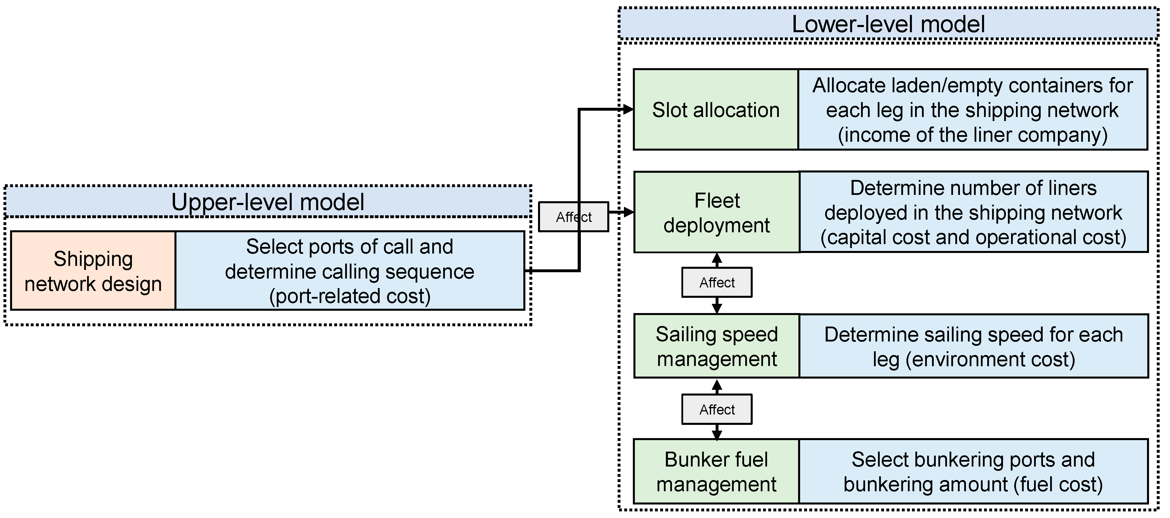
On the basis of the above concepts, we propose a systematic modeling framework for LSSD for methanol-powered vessels. The modeling framework aims to achieve the joint optimization of four core decision-making issues: (1) fleet deployment (including sailing speed management), (2) shipping network design, (3) slot allocation, and (4) bunker fuel management. The above shipping network design constitutes the foundation of the entire modeling framework. The primary task is to determine the ports of call and the calling sequence. By employing a scientific approach to the selection of hub (feeder) ports and the formulation of legs, an efficient shipping network can be constructed, thereby maximizing the profit of the liner company. Building on this foundation, the slot allocation decision focuses on optimizing the allocation of liner slots to increase system operational efficiency. In addition, sailing speed management concentrates on determining the optimal speed for each leg of the route, which also determines the number of liners deployed in the shipping network. Given the nonlinear relationship between fuel consumption and sailing speed, bunker fuel management also needs to be considered simultaneously. Based on the above analysis, we present a bi-level optimization model framework, as shown in Figure 2. For the convenience of readers, we list the commonly used notations in

Table 1. Notation table.

Sets
P	Set of all candidate ports of call, indexed by i or j
$N$	Set of all shipping network design schemes, indexed by n
$K$	Set of fuel type, indexed by k
$S$	Set of liner class, indexed by s
$B(i,j,n)$	$\mathrm{Set} \mathrm{of} \mathrm{all} \mathrm{possible} \mathrm{transportation} \mathrm{paths} \mathrm{associated} \mathrm{with} \mathrm{OD} \mathrm{pair} d(i,j)$ in the shipping network design scheme $n$, indexed by b
$V\left(n\right)$	Set of ports of call associated with network design scheme n
$E\left(n\right)$	$\mathrm{Set} \mathrm{of} \mathrm{legs} \mathrm{in} \mathrm{network} \mathrm{design} \mathrm{scheme} n, \mathrm{represented} \mathrm{as} \left[i,j\right]$
${\delta }_n^{+}\left(i\right)$	Set of legs whose head node is port i in network design scheme n
${\delta }_n^{-}\left(i\right)$	Set of legs whose tail node is port i in network design scheme n
Parameters
$d(i,j)$	OD pair with origin port i and destination port j
$D(i,j)$	$\mathrm{Transportation} \mathrm{demand} \mathrm{associated} \mathrm{with} \mathrm{OD} \mathrm{pair} d(i,j)$
$r(i,j)$	$\mathrm{Freight} \mathrm{rate} \mathrm{associated} \mathrm{with} \mathrm{OD} \mathrm{pair} d(i,j)$
$c_L(i,j,b)$	$\mathrm{Cost} \mathrm{incurred} \mathrm{by} \mathrm{the} \mathrm{liner} \mathrm{company} \mathrm{for} \mathrm{transporting} \mathrm{one} \mathrm{TEU} \mathrm{of} \mathrm{laden} \mathrm{container} \mathrm{from} \mathrm{port} i \mathrm{to} \mathrm{port} j\mathrm{on} \mathrm{transportation} \mathrm{path} b\in B(i,j,n)$ in shipping network design scheme $n$
$c_E(i,j,b)$	$\mathrm{Cost} \mathrm{incurred} \mathrm{by} \mathrm{the} \mathrm{liner} \mathrm{company} \mathrm{for} \mathrm{transporting} \mathrm{one} \mathrm{TEU} \mathrm{of} \mathrm{empty} \mathrm{container} \mathrm{from} \mathrm{port} i \mathrm{to} \mathrm{port} j\mathrm{on} \mathrm{transportation} \mathrm{path} b\in B(i,j,n)$ in shipping network design scheme $n$
$d_{is}(\left[i,j\right],n)$	$\mathrm{Distance} \mathrm{of} \mathrm{leg} \left[i,j\right]$ in network design scheme $n$
$\delta (\left[i,j\right],l,m,b)$	$\text{Leg-path} \mathrm{indicator} \mathrm{that} \mathrm{is} 1 \mathrm{if} \mathrm{the} \mathrm{transportation} \mathrm{path} b \mathrm{associated} \mathrm{with} \mathrm{OD} \mathrm{pair} d(l,m)\mathrm{contains} \mathrm{leg} \left[i,j\right]$, and 0 otherwise
$h\left(i\right)$	Liner berthing time at port i
$p_k\left(i\right)$	$\mathrm{Price} \mathrm{of} \mathrm{unit} \mathrm{type} k\in K$ fuel at port i
${\tau }_i$$, {{\tau }^{\prime }}_{i,j}$	$\mathrm{Carbon} \mathrm{tax} \mathrm{rate} \mathrm{set} \mathrm{by} \mathrm{the} \mathrm{government} \mathrm{where} \mathrm{port} i \mathrm{or} \mathrm{leg} \left[i,j\right]$ is located
${\gamma }_k$	Fuel consumption–carbon emission conversion factor for type k fuel
${\alpha }_k$$, {\beta }_k$	Fuel consumption coefficient associated with type k fuel
$E_k^{\min }$	Minimum fuel inventory required for fuel tank of a class k liner
$E_k$	Capacity of fuel tank for a class k liner
$Q$	Liner capacity
$v_{\min }$$, v_{\max }$	Minimum/maximum sailing speed allowed
$f_p(i,n)$	Fuel consumption at port i in shipping network design scheme n
$C_s$	Annual construction (i.e., purchase) cost for a class s liner
$C_i^{\mathrm{F}}$	Fixed cost incurred by liner bunkers at the port i
Decision variables
$y\left(n\right)$	Binary variable, 1, if shipping network design scheme $n$ is selected by the liner company, 0 otherwise
$z(i,n)$	Binary variable, 1 if port i is selected for bunkering in shipping network design scheme n, 0 otherwise
$v(\left[i,j\right],n)$	$\mathrm{Average} \mathrm{sailing} \mathrm{speed} \mathrm{on} \mathrm{leg} \left[i,j\right]$ in shipping network design scheme $n$
$q(i,n)$	Bunkering amount at port i in shipping network design scheme n
$e(i,n)$	Fuel inventory after bunkering at port i in shipping network design scheme n
$x(\left[i,j\right],n)$	$\mathrm{Total} \mathrm{container} \mathrm{flow} \mathrm{volume} \mathrm{on} \mathrm{leg} \left[i,j\right]$ in shipping network design scheme n
$x_L(i,j,n)$	$\mathrm{Laden} \mathrm{container} \mathrm{flow} \mathrm{volume} \mathrm{associated} \mathrm{with} \mathrm{OD} \mathrm{pair} d(i,j)$ in shipping network design scheme $n$
$x_L(i,j,b,n)$	$\mathrm{Laden} \mathrm{container} \mathrm{flow} \mathrm{volume} \mathrm{on} \mathrm{transportation} \mathrm{path} b\in B(i,j,n)$  $\mathrm{associated} \mathrm{with} \mathrm{OD} \mathrm{pair} d(i,j)$ in shipping network design scheme $n$
$x_E(i,j,n)$	$\mathrm{Empty} \mathrm{container} \mathrm{flow} \mathrm{volume} \mathrm{associated} \mathrm{with} \mathrm{OD} \mathrm{pair} d(i,j)$ in shipping network design scheme $n$
$x_E(i,j,b,n)$	$\mathrm{Empty} \mathrm{container} \mathrm{flow} \mathrm{volume} \mathrm{on} \mathrm{transportation} \mathrm{path} b\in B(i,j,n)$  $\mathrm{associated} \mathrm{with} \mathrm{OD} \mathrm{pair} d(i,j)$ in shipping network design scheme $n$
$a\left(n\right)$	Number of liners deployed in the liner fleet
$f(\left[i,j\right],n)$	$\mathrm{Fuel} \mathrm{consumption} \mathrm{on} \mathrm{leg} \left[i,j\right]$ in shipping network design scheme $n$

.

4. Model Establishment

In this section, we develop the model to achieve the mathematical modeling of the problem. To this end, we first give basic assumptions in Section 4.1 to simplify the problem. Then, Section 4.2 gives the expression of the model.

4.1. Model Assumptions

This paper makes the following assumptions based on shipping practices.

• Shipping network structure: The shipping network consists of one trunk route (which connects hub ports and operates in a closed-loop manner) and several feeder routes (which employs a hub-and-spoke structure to connect hub ports with feeder ports). We assume that the liner company is responsible solely for the operation of trunk routes, whereas feeder routes are operated by independent feeder liner companies [1,21].
• Liner operations: We assume that the liners deployed in the fleet have the same class (i.e., capacity) and that the liner class is known. The calling frequency is set to once a week [1,20]. This assumption can be relaxed by introducing a decision variable associated with the calling frequency. Therefore, this assumption does not affect the structure of the model. All the liners deployed in this fleet sail at the same speed when they are on the same leg (e.g., leg “Port A → Port B”). However, the sailing speed may vary between different legs. The minimum and maximum sailing speeds of various types of liners are fixed and known. The liner berthing time at each port of call is fixed at 18 h.
• Bunkering feel management: The fuel price is known and fixed at each port of call, and liner companies can choose to bunker with either traditional fuel or methanol [28,42]. This assumption is introduced because the planning period of LSSD is usually 3 to 6 months, and the fuel price does not change significantly [1,21]. Moreover, liner companies usually sign agreements to guarantee stable fuel prices for a period of time to control costs in practice. Traditional fuels can be classified into several categories. For the convenience of modeling, we assume that the traditional fuel used by the liner company is very-low-sulfur fuel oil (VLSFO). The liner only bunkers at the port of call, with bunkering time included in the berthing time. To ensure navigational safety, the minimum fuel inventory in the liner’s fuel tank is set at 10% of the tank capacity.
• Fuel consumption: Owing to the lack of operational data on methanol-powered liners, we can establish a fuel consumption correction factor for methanol-powered liners that aligns with the consumption levels of HFO-powered liners. This correction factor is adjusted on the basis of the ratio of the energy density of methanol (19.9 MJ/kg) to that of HFO (40.2 MJ/kg).
• Container: in the context of container transportation, we assume that all containers transported along the shipping network are twenty feet equivalent units (TEUs), with other container sizes converted into TEUs.

4.2. Model Development

In this paper, we use a bi-level optimization framework to achieve the mathematical modeling of the problem, where the upper-level model optimizes the number of liners deployed in the fleet and shipping network structure, and the lower-level model coordinates decisions regarding liner sailing speed management, bunker fuel management, and slot allocation.

4.2.1. Upper-Level Model

The upper-level model addresses shipping network design by determining the hub ports, feeder ports, and calling sequence. Before modeling, we first introduce some notation. Let $R\left(n\right)$ and $C\left(n\right)$ represent the income and cost associated with shipping network design scheme n, respectively. They are calculated using the lower-level model. $y\left(n\right)$ is a binary variable. It takes a value of 1 if shipping network design scheme $n$ is selected by the liner company, and 0 otherwise.

Upper-level model:

$$\max {\displaystyle \sum _{n\in N}y\left(n\right)\left[R\left(n\right)-C\left(n\right)\right]}$$

(1)

$$s.t. {\displaystyle \sum _{n\in N}y\left(n\right)}=1$$

(2)

$$y\left(n\right)\in \left\{0,1\right\}.$$

(3)

The objective function is defined as Equation (1), which is used to calculate the profit of the liner company. Constraint (2) requires that the liner company can select only one element (i.e., shipping network design scheme) from N to be executed. Finally, Constraint (3) is a binary constraint affecting the decision variable $y\left(n\right)$.

4.2.2. Lower-Level Model

Based on the shipping network structure, determined by the upper-level model (with scheme n known), the lower-level model can be developed as follows. Before introducing the model, we first give the notation definitions used in the model. In order to carry out comparative experiments, we let $K$ represent the set of fuel types, and its element is denoted as $k$; $S$ denotes the set of liner classes, and its element is denoted as $s$. When the lower model is solved, the optimal results for different types of fuel (or classes of liners) can be calculated by changing the value of k (or s). In addition, we let $r\left(i,j\right)$ denote the freight rate associated with the OD pair $d\left(i,j\right)$; $c_L\left(i,j,b\right)$ and $c_E\left(i,j,b\right)$ represent the costs incurred by the liner company for transporting one TEU of laden container and one TEU of empty container from port i to port j on transportation path $b\in B\left(i,j,n\right)$ in shipping network design scheme $n$; and $p_k\left(i\right)$ represents the price of unit type $k\in K$ fuel at port i. $q\left(i,n\right)$ denotes the bunkering amount at port i in shipping network design scheme $n$. $C_i^{\mathrm{F}}$ represents the fixed cost incurred by liner bunkers at port $i$. $z\left(i,n\right)$ denotes a binary variable. If port $i$ is selected for bunkering in shipping network design scheme $n$, it takes a value of 1 and takes 0 otherwise. $Q$ is the liner capacity. $C_s$ denotes the construction (i.e., purchase) cost for a class s liner. $a\left(n\right)$ denotes the number of liners deployed in the liner fleet. ${\tau }_i$ and ${{\tau }^{\prime }}_{i,j}$ represent the carbon tax rate set by the government where port i or leg $\left[i,j\right]$ is located. ${\gamma }_k$ is the fuel consumption–carbon emission conversion factor for type $k$ fuel. $f\left(\left[i,j\right],n\right)$ and $f_p\left(i,n\right)$ denote the fuel consumption on leg $\left[i,j\right]$ and at port i in the shipping network design scheme $n$, respectively. $\delta \left(\left[i,j\right],l,m,b\right)$ represents a leg-path indicator of 1 if transportation path b associated with OD pair $d\left(l,m\right)$ contains leg $\left[i,j\right]$ and one of 0 otherwise. ${\delta }_n^{+}\left(i\right)$ and ${\delta }_n^{-}\left(i\right)$ are sets of legs whose head and tail nodes are port i in network design scheme $n$, respectively. $D\left(i,j\right)$ is the transportation demand associated with the OD pair $d\left(i,j\right)$. $d_{is}\left(\left[i,j\right],n\right)$ denotes the distance of leg $\left[i,j\right]$ in network design scheme $n$. $v\left(\left[i,j\right],n\right)$ represents the average sailing speed on leg $\left[i,j\right]$ in network design scheme $n$. $h\left(i\right)$ is the liner berthing time at port i. $a\left(n\right)$ represents the number of liners deployed in the liner fleet. $e\left(i,n\right)$ denotes the fuel inventory after bunkering at port i in the shipping network design scheme $n$. $E_k$ is the capacity of the fuel tank for a type k liner. $E_k^{\min }$ denotes the minimum fuel inventory required for the fuel tank of a type k liner. ${\alpha }_k$ and ${\beta }_k$ are fuel consumption coefficients. Finally, $v_{\min }$ and $v_{\max }$ denote the minimum and maximum sailing speeds allowed, respectively.

Lower-level model:

$$\max R\left(n\right)-C\left(n\right)$$

(4)

$$s.t. R\left(n\right)={\displaystyle \sum _{i,j\in V\left(n\right),i\ne j}{\displaystyle \sum _{b\in B\left(i,j,n\right)}\left\{\begin{array}{l}\left[r\left(i,j\right)-c_L\left(i,j,b\right)\right]x_L\left(i,j,b,n\right)\\ -c_E\left(i,j,b\right)x_E\left(i,j,b,n\right)\end{array}\right\}}}$$

(5)

$$\mathrm{C}\left(n\right)=\left\{\begin{array}{c}\mathrm{Fuel} \mathrm{cost}\left(n\right)+\mathrm{Port} \mathrm{related} \mathrm{cost}\left(n\right)+\mathrm{Capital} \mathrm{cost}\left(n\right)\\ +\mathrm{Operational} \mathrm{cost}\left(n\right)+\mathrm{Environmental} \mathrm{cost}\left(n\right)\end{array}\right\}$$

(6)

$$\mathrm{Fuel} \mathrm{cost}\left(n\right)={\displaystyle \sum _{i\in V\left(n\right)}\left[p_k\left(i\right)q\left(i,n\right)+C_i^{\mathrm{F}}z\left(i,n\right)\right]}$$

(7)

$$\mathrm{Port} \mathrm{related} \mathrm{cost}\left(n\right)=\left|V\left(n\right)\right|\left(1.95Q+5200\right)$$

(8)

$$\mathrm{Capital} \mathrm{cost}\left(n\right)={\displaystyle \frac{C_s}{52\times 10}}a\left(n\right)$$

(9)

$$\mathrm{Operational} \mathrm{cost}\left(n\right)=0.5\times \mathrm{Capital} \mathrm{cost}\left(n\right)$$

(10)

$$\text{Environmental cost}\left(n\right)={\displaystyle \sum _{i\in V\left(n\right)}{\tau }_i{\gamma }_k{f}_p\left(i,n\right)}+{\displaystyle \sum _{\left[i,j\right]\in E\left(n\right)}{\tau }_{i,j}^{\prime }{\gamma }_{k}f\left(\left[i,j\right],n\right)}$$

(11)

$$x_L\left(i,j,n\right)={\displaystyle \sum _{b\in B\left(i,j,n\right)}{x}_L\left(i,j,b,n\right)}; \forall i,j\in V\left(n\right),i\ne j$$

(12)

$$x_E\left(i,j,n\right)={\displaystyle \sum _{b\in B\left(i,j,n\right)}{x}_E\left(i,j,b,n\right)}; \forall i,j\in V\left(n\right),i\ne j$$

(13)

$$x\left(\left[i,j\right],n\right)={\displaystyle \sum _{l,m\in V\left(n\right),l\ne m}{\displaystyle \sum _{b\in B\left(k,l,n\right)}\left[x_L\left(l,m,b,n\right)+x_E\left(l,m,b,n\right)\right]\delta \left(\left[i,j\right],l,m,b\right)}}; \forall \left[i,j\right]\in E\left(n\right)$$

(14)

$${\displaystyle \sum _{\left[i,j\right]\in {\delta }_n^{-}\left(i\right)}x\left(\left[i,j\right],n\right)}={\displaystyle \sum _{\left[j,i\right]\in {\delta }_n^{+}\left(i\right)}x\left(\left[j,i\right],n\right)}; \forall i\in V\left(n\right)$$

(15)

$$x\left(\left[i,j\right],n\right)\le Q; \forall \left[i,j\right]\in E\left(n\right)$$

(16)

$$x_L\left(i,j,n\right)\le D\left(i,j\right); \forall i,j\in V\left(n\right),i\ne j$$

(17)

$${\displaystyle \sum _{\left[i,j\right]\in E\left(n\right)}\frac{d_{is}\left(\left[i,j\right],n\right)}{v\left(\left[i,j\right],n\right)}}+{\displaystyle \sum _{i\in V\left(n\right)}h}\left(i\right)\le 7\times a\left(n\right)$$

(18)

$$q\left(j,n\right)=e\left(j,n\right)-e\left(i,n\right)+f_p\left(j,n\right)+f\left(\left[i,j\right],n\right); \forall \left[i,j\right]\in E\left(n\right)$$

(19)

$$z\left(i,n\right)E_k^{\min }\le q\left(i,n\right)\le z\left(i,n\right)E_k; \forall i\in V\left(n\right)$$

(20)

$$e\left(i,n\right)\le E_k; \forall i\in V\left(n\right)$$

(21)

$$e\left(i,n\right)\ge E_k^{\min }+f\left(\left[i,j\right],n\right); \forall \left[i,j\right]\in E\left(n\right)$$

(22)

$$f\left(\left[i,j\right],n\right)={\alpha }_k{d}_{is}\left(\left[i,j\right],n\right)v{\left(\left[i,j\right],n\right)}^{{\beta }_k-1}/24; \forall \left[i,j\right]\in E\left(n\right)$$

(23)

$$v_{\min }\le v\left(\left[i,j\right],n\right)\le v_{\max }; \forall \left[i,j\right]\in E\left(n\right)$$

(24)

$$z\left(i,n\right)\in \left\{0,1\right\}; \forall i\in V\left(n\right)$$

(25)

$$a\left(n\right)\in {\mathbb{Z}}_{+}$$

(26)

$$x_L\left(i,j,b,n\right)\ge 0,x_E\left(i,j,b,n\right)\ge 0; \forall i,j\in V\left(n\right),i\ne j,b\in B\left(i,j,n\right)$$

(27)

$$v\left(\left[i,j\right],n\right)\ge 0; \forall \left[i,j\right]\in E\left(n\right)$$

(28)

$$q\left(i,n\right)\ge 0,e\left(i,n\right)\ge 0; \forall i\in V\left(n\right).$$

(29)

In the above, Equation (4) is the objective function, which calculates the profit of the liner company when selecting the shipping network design scheme $n$. Constraint (5) calculates the weekly income from transportation containers. Constraint (6) calculates the total weekly costs under shipping network design scheme n, which includes fuel costs, port-related costs, capital costs, operational costs, and environmental costs. Constraints (7)–(11) show how to calculate different types of costs. Constraints (8) and (9) are referenced from Xiang, Xin, Zhang, Chen, and Liu [21]. Assuming that the capital cost of a liner is spread over 10 years, with 52 weeks per year, the weekly capital cost can be calculated using Constraint (9). Constraint (12) establishes the relationship between $x_L\left(i,j,n\right)$ and $x_L\left(i,j,b,n\right)$. Similarly, Constraint (13) gives the relationship between $x_E\left(i,j,n\right)$ and $x_E\left(i,j,b,n\right)$. The above two constraints indicate that the laden (empty) container flow volume associated with the OD pair $d\left(i,j\right)$ is equal to the sum of the flows along each transportation path associated with the OD pair $d\left(i,j\right)$. Constraint (14) gives the relationship between the container flow volume associated with leg $\left[i,j\right]$ and the container flow volume associated with the OD pair, i.e., $x_L\left(k,l,b,n\right)$ and $x_E\left(k,l,b,n\right)$. Constraint (15) ensures that the number of containers (both laden and empty) flowing into each port of call is equal to the number of containers (both heavy and empty) flowing out of this port of call. This effectively ensures that the number of containers in each port of call is balanced. Constraint (16) ensures that the total container flow volume on each leg does not exceed the liner’s capacity. Constraint (17) indicates that the container transportation volume associated with the OD pair $d\left(i,j\right)$ does not exceed the transportation demand. Constraint (18) ensures that the liners can maintain a stable calling frequency. Constraint (19) calculates the amount of liner bunkering at port j. Constraint (20) ensures that the liner bunkering amount at port i does not exceed the maximum capacity of the tank and is not less than the lower limit of fuel inventories. Constraint (21) limits the fuel inventory after bunkering at port i so that it does not exceed the tank capacity. Constraint (22) ensures that, after bunkering at port i, the liner can navigate to the next port j. Constraint (23) calculates fuel consumption for leg $\left[i,j\right]$. Constraint (24) specifies the arrival time of the liner at port j. Constraint (24) is used to restrict the liner sailing speed within the prescribed limits. Constraints (25)–(29) show the domains of the decision variables in the lower-level model.

5. Solution Methodology

This section introduces the algorithm design idea used in LSSD for methanol-powered vessels. Owing to the involvement of several sub-problems, the problem discussed in this paper is essentially a compounding of the traveling salesman problem and the knapsack problem [21]. Therefore, LSSD for methanol-powered vessels is an NP-hard problem. We also cannot find an efficient algorithm unless P equals NP. Although we cannot enumerate all the elements in set N, it is easy to evaluate their performance. This suggests that we can use meta-heuristics to encode the elements in set N (shipping network design schemes) and then obtain the fitness of individuals (elements) by solving the underlying model. Moreover, an examination of the lower-level model reveals that the decision variables can be divided into two mutually independent groups. The first group pertains to fleet deployment (with sailing speed management) and bunker fuel management, whereas the second group concerns slot allocation. This feature allows the calculation of individual fitness values to be divided into two independent optimization problems.

• For the encoding of the shipping network design scheme, we can use the optimal fleet deployment (with sailing speed management) and bunker fuel management strategies to achieve the lowest costs.
• For the encoding of the shipping network design scheme, we can optimize the slot allocation scheme to maximize profit.

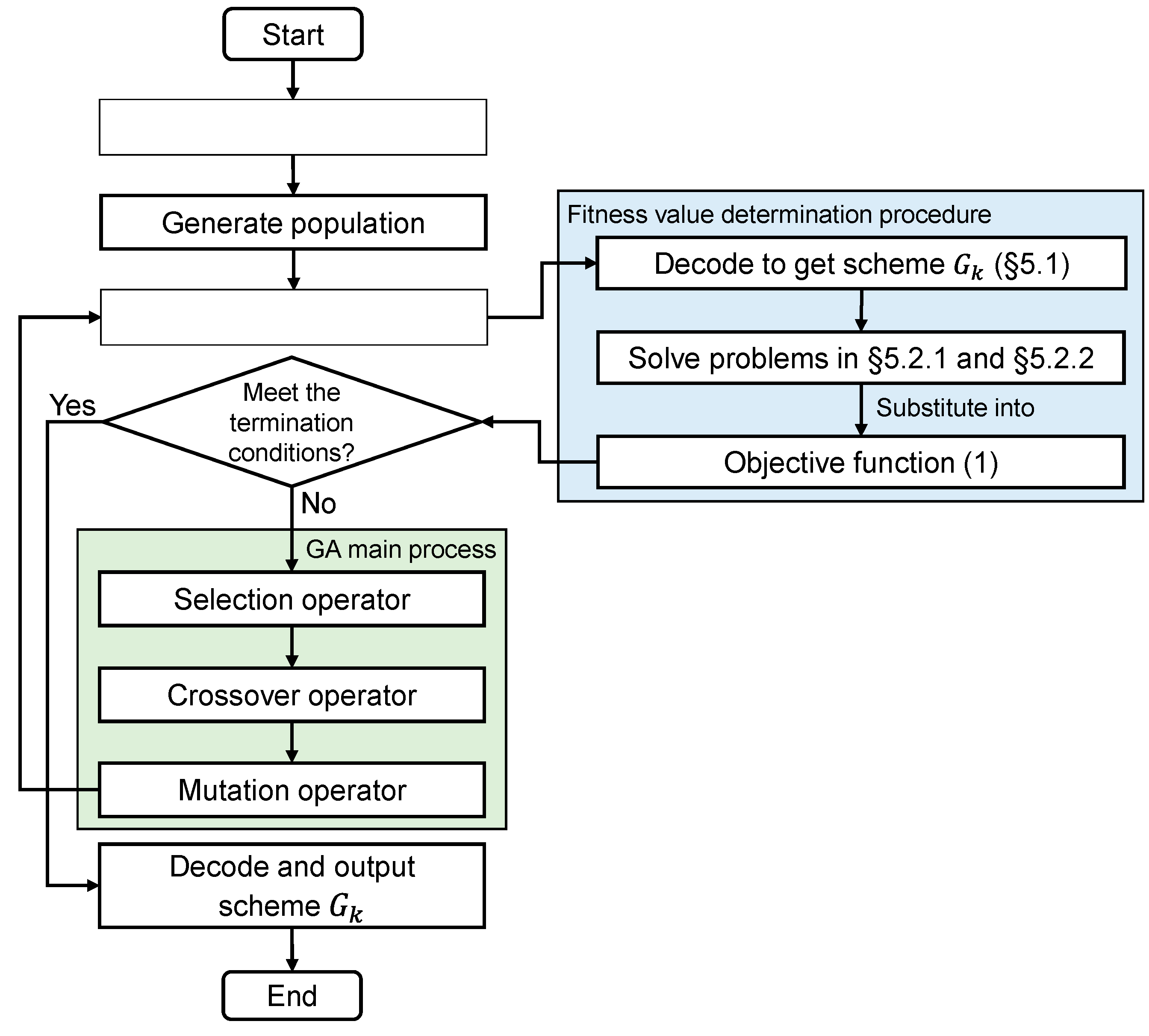
This decomposition strategy significantly reduces the difficulty of solving the problem. In this context, we propose a meta-heuristic algorithm based on the GA framework to solve the model. In the following subsections, we first introduce the encoding and decoding methods and then detail the piecewise linearization method, used for the nonlinear constraints in the lower-level model. We use Figure 3 to represent the overall framework of the algorithm.

5.1. Encoding and Decoding Methods

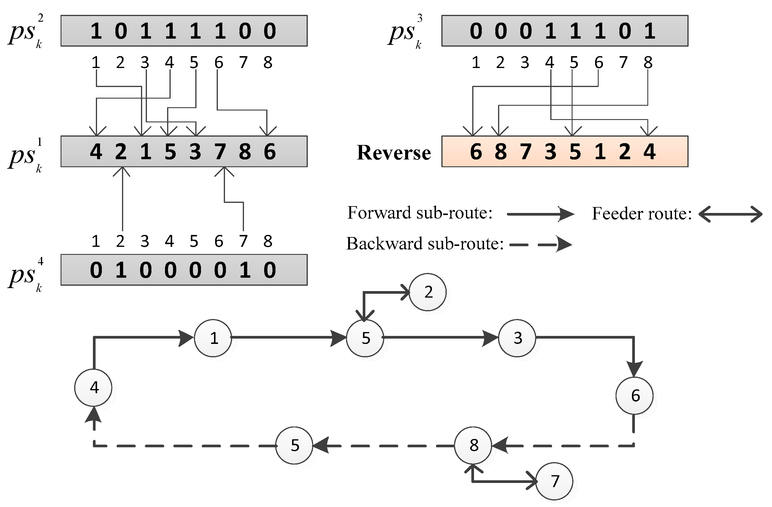
The encoding of the shipping network design scheme is a key procedure in employing a GA. An effective encoding scheme should not only comprehensively represent the structural characteristics of the shipping network but also facilitate genetic operations. In this paper, we encode the shipping network design scheme n into a chromosome containing four gene sequences (i.e., $p{s}_k^1$ to $p{s}_k^4$). Specifically, sequence $p{s}_k^1$ represents a random permutation of integers from 1 to $\left|P\right|$, where $P$ is the set of alternative ports of call. In this way, each alternative port of call can be represented by a unique integer (e.g., Port 2, Port 7). The sequences $p{s}_k^2$, $p{s}_k^3$, and $p{s}_k^4$ are binary-coded sequences of length $\left|P\right|$. Figure 4 illustrates the complete encoding and decoding process. The decoding process can be divided into three steps: (1) determining the forward sub-route of the trunk route, (2) determining the backward sub-route of the trunk route, and (3) determining the feeder route. In the case illustrated in Figure 2, the four gene sequences of a chromosome are as follows:

$$p{s}_k^1=\left(4 2 1 5 3 7 8 6\right), p{s}_k^2=\left(1 0 1 1 1 1 0 0\right),$$

$$p{s}_k^3=\left(0 0 0 1 1 1 0 1\right)\mathrm{and} p{s}_k^4=\left(0 1 0 0 0 0 1 0\right).$$

The specific decoding process is as follows. During encoding, some infeasible chromosomes (infeasible solutions) may be generated, and gene repair operations need to be performed. We adopt the gene repair scheme proposed by Xiang, Xin, Zhang, Chen, and Liu [21] and Chen, Yi, Xin, and Zhang [1] and do not provide details here.

Decoding process 1: This involves determining the forward sub-route of the trunk route. Based on sequence $p{s}_k^2$, the value for gene loci 1, 3, 4, 5, and 6 is 1, whereas the value for other gene loci is 0. This indicates that ports 1, 3, 4, 5, and 6 are selected as the ports of call in the forward sub-route. According to the order in which these ports appear in sequence $p{s}_k^1$ (from left to right), the calling sequence of ports 1, 3, 4, 5, and 6 can be determined as 4, 1, 5, 3, and 6. Therefore, the forward sub-route of the trunk route is designated “$4\to 1\to 5\to 3\to 6$”.

Decoding process 2: This involves determining the backward sub-route of the trunk route. Based on the sequence $p{s}_k^3$, the value for gene loci 4, 5, and 6 is 1, whereas that for the other gene loci is 0. This indicates that ports 4, 5, 6, and 8 are selected as the ports of call in the backward sub-route. According to the order in which these ports appear in sequence $p{s}_k^1$ (from right to left, opposite to decoding process 1), the calling sequence can be determined as 6, 8, 5, and 4. Thus, the backward sub-route of the trunk route is designated “$6\to 8\to 5\to 4$”.

Decoding process 3: This involves determining the feeder route. On the basis of the sequence $p{s}_k^4$, the value for gene loci 2 and 7 is 1, whereas that for other gene loci is 0. This indicates that ports 2 and 7 are selected as the feeder ports. Each feeder port needs to be connected to a specific hub port (i.e., the port included in the truck route) to form two bidirectional legs. Working according to the principle of minimizing transportation costs, the connection relationships between the feeder ports and trunk ports are determined. We assume that the transportation cost from Port 2 to Port 5 is the lowest and that the transportation cost from Port 7 to Port 8 is also the lowest. Thus, two feeder routes are obtained, i.e., “$2\leftrightarrow 5$” and “$7\leftrightarrow 8$”.

5.2. Fitness Value Calculation

The fitness calculation within the LSSD problem involves two mutually independent optimization sub-problems. This section provides a detailed explanation of the solution methods used for these two sub-problems.

5.2.1. Optimization of Sailing Peed and Bunkering Fuel Management Strategies

A nonlinear relationship exists between sailing speed and fuel consumption. To increase the solution’s efficiency, we employ a method that integrates reciprocal transformation and adaptive piecewise linear approximation. The process consists of the following five steps:

Step 1: Reciprocal transformation. The decision variable $v\left(\left[i,j\right],n\right)$ undergoes reciprocal transformation to reformulate the relevant nonlinear constraints. For example, several key constraints in the model (e.g., Constraints (18), (23), and (24)) are transformed via a reciprocal method, i.e., $v\left(\left[i,j\right],n\right)\to 1/\pi \left(\left[i,j\right],n\right)$, to facilitate more efficient linearization in subsequent steps. The reconstructed constraints are shown in Equations (30)–(32) below.

$${\displaystyle \sum _{\left[i,j\right]\in E\left(n\right)}{d}_{is}\left(\left[i,j\right],n\right)}\pi \left(\left[i,j\right],n\right)+{\displaystyle \sum _{i\in V\left(n\right)}h}\left(i\right)\le 7\times a\left(n\right)$$

(30)

$$f\left(\pi \left(\left[i,j\right],n\right)\right)={\alpha }_k{d}_{is}\left(\left[i,j\right],n\right){\left[1/\pi \left(\left[i,j\right],n\right)\right]}^{{\beta }_k-1}/24; \forall \left[i,j\right]\in E\left(n\right)$$

(31)

$${\displaystyle \frac{1}{v_{\min }}}\le \pi \left(\left[i,j\right],n\right)\le {\displaystyle \frac{1}{v_{\max }}}; \forall \left[i,j\right]\in E\left(n\right)$$

(32)

Step 2: Linear approximation using the convexity of the fuel consumption function. The nonlinear component in Constraint (23) is the only nonlinear constraint used in the lower-level model. Based on the convexity of the fuel consumption function, we employ an adaptive piecewise linear approximation method to reformulate this constraint. To ensure that the approximation error remains within acceptable limits, the intervals of the fuel consumption function are initially divided, and the fuel consumption of the liner on each leg is linearized. Specifically, to guarantee that the approximation error is acceptable, we define an error value $\psi$ and preliminarily divide the interval $\left[G_{\min },G_{\max }\right]$, where $G_{\max }=1/v_{\min }$ and $G_{\min }=1/v_{\max }$. Within this interval, the liner fuel consumption limits for each leg are obtained, with the upper bound given by Equation (33) and the lower bound by Equation (34).

$$f{\left(\left[i,j\right],n\right)}_{\max }={\alpha }_k{d}_{is}\left(\left[i,j\right],n\right){\left(1/G_{\min }\right)}^{{\beta }_k-1}/24; \forall \left[i,j\right]\in E\left(n\right)$$

(33)

$$f{\left(\left[i,j\right],n\right)}_{\min }={\alpha }_k{d}_{is}\left(\left[i,j\right],n\right){\left(1/G_{\max }\right)}^{{\beta }_k-1}/24; \forall \left[i,j\right]\in E\left(n\right)$$

(34)

Step 3: Piecewise linearization and error control. In this step, we divide the domain of the fuel consumption function into several segments of equal length, and a piecewise linear function for fuel consumption is calculated at each of these division points. The fuel consumption within each segment (i.e., a subset of the domain) is estimated via Equation (36). If the approximation error for a segment does not meet the error requirements, then this segment is further subdivided to ensure that the approximation error remains within acceptable limits. Specifically, the interval $\left[G_{\min },G_{\max }\right]$ is initially divided into $u$ interval segments of equal length. At division point z ($z=0,1,\dots ,u$), we directly set the value of $\pi {\left(\left[i,j\right],n\right)}_z$ to $\left[z/u\left(G_{\max }-G_{\min }\right)\right]+G_{\min }$; thus, the fuel consumption function at division point z can be expressed as shown in Equation (35).

$$f\left(\pi {\left(\left[i,j\right],n\right)}_z\right)={\alpha }_k{d}_{is}\left(\left[i,j\right],n\right){\left\{1/\left[z/u\left(G_{\max }-G_{\min }\right)+G_{\min }\right]\right\}}^{{\beta }_k-1}/24; \forall z\in \left\{0,1,\dots ,u\right\},\left[i,j\right]\in E\left(n\right)$$

(35)

Moreover, if $\pi \left(\left[i,j\right],n\right)$ takes values within segment $\left[\pi {\left(\left[i,j\right],n\right)}_z,\pi {\left(\left[i,j\right],n\right)}_{z+1}\right)$, where $z=0,1,\dots ,\left(u-1\right)$, then the piecewise linear reformulation for the fuel consumption function can be expressed as Equation (36).

$$\tilde{f}\left[\pi \left(\left[i,j\right],n\right)\right]=f\left[\pi {\left(\left[i,j\right],n\right)}_z\right]+{\displaystyle \frac{\left[\pi \left(\left[i,j\right],n\right)-\pi {\left(\left[i,j\right],n\right)}_z\right]}{\left(G_{\max }-G_{\min }\right)/u}}\left\{f\left[\pi {\left(\left[i,j\right],n\right)}_{z+1}\right]-f\left[\pi {\left(\left[i,j\right],n\right)}_z\right]\right\}; \forall \left[i,j\right]\in E\left(n\right)$$

(36)

Step 4: The refinement and convergence of the approximation errors. During the error control process, the segments that do not meet the accuracy requirements are progressively refined until the approximation errors for all segments comply with the requirements of Equation (37). This process ensures that the precision of piecewise linearization meets the computational needs (i.e., $\psi$), ultimately replacing the nonlinear terms (or constraints) in the model with linear terms (or constraints). Specifically, for each segment within interval $\left[G_{\min },G_{\max }\right]$, a check is performed to determine whether the following equation holds:

$$\underset{z\in \left\{0,1,\mathrm{\dots },u-1\right\}}{\max }\left\{\left|\frac{\frac{f\left[\pi {\left(\left[i,j\right],n\right)}_z\right]+f\left[\pi {\left(\left[i,j\right],n\right)}_{z+1}\right]}{2}-f\left(\frac{\pi {\left(\left[i,j\right],n\right)}_z+\pi {\left(\left[i,j\right],n\right)}_{z+1}}{2}\right)}{f\left(\frac{\pi {\left(\left[i,j\right],n\right)}_z+\pi {\left(\left[i,j\right],n\right)}_{z+1}}{2}\right)}\right|\right\}\le \psi ; \forall \left[i,j\right]\in E\left(n\right).$$

(37)

If one segment fails to satisfy Equation (37), the approximation error for that particular segment can be inferred to be excessive. This consequently necessitates the subdivision of the segment to reduce the aforementioned error and thereby ensure that the approximation error of each segment meets the minimum error requirements. For example, when the approximation error for segment $\left[\pi {\left(\left[i,j\right],n\right)}_z,\pi {\left(\left[i,j\right],n\right)}_{z+1}\right]$ does not meet the minimum error requirement (i.e., does not satisfy Equation (37)), then we should return to Step 3 to re-divide interval $\left[G_{\min },G_{\max }\right]$ by setting $u=u+1$.

Step 5: Construct the linearized model. Through the aforementioned processes, a linearized optimization model is obtained. The final piecewise linear Equations (36) and (37) replace the nonlinear Equation (23) in the original lower-level model, whereas Constraints (30)–(32) replace the corresponding constraints in the original lower-level model. After these transformations, the nonlinear lower-level model is simplified into a mixed-integer linear programming model, significantly reducing the computational difficulty and resulting in a new lower-level model.

5.2.2. The Optimization of the Slot Allocation Scheme

Based on the shipping network design scheme, the optimization of the slot allocation scheme focuses primarily on the allocation of laden and empty containers to different legs. This problem is essentially a network flow problem, with the objective of maximizing container transportation profit earned by the liner company. Given that all constraints of the problem are linear and that the decision variables are continuous, this optimization problem can be directly formulated as a linear programming model. On the basis of the lower-level model, we present a mathematical model of the slot allocation problem, which is composed of parts of the lower-level model. For the completeness of the model, we repeat some of the previous constraints.

$$\max {\displaystyle \sum _{i,j\in V\left(n\right),i\ne j}{\displaystyle \sum _{b\in B\left(i,j,n\right)}\left\{\begin{array}{l}\left[r\left(i,j\right)-c_L\left(i,j,b\right)\right]x_L\left(i,j,b,n\right)\\ -c_E\left(i,j,b\right)x_E\left(i,j,b,n\right)\end{array}\right\}}}$$

(38)

$$s.t. x_L\left(i,j,n\right)={\displaystyle \sum _{b\in B\left(i,j,n\right)}{x}_L\left(i,j,b,n\right)}; \forall i,j\in V\left(n\right),i\ne j$$

(39)

$$x_E\left(i,j,n\right)={\displaystyle \sum _{b\in B\left(i,j,n\right)}{x}_E\left(i,j,b,n\right)}; \forall i,j\in V\left(n\right),i\ne j$$

(40)

$$x\left(\left[i,j\right],n\right)={\displaystyle \sum _{l,m\in V\left(n\right),l\ne m}{\displaystyle \sum _{b\in B\left(k,l,n\right)}\left[x_L\left(l,m,b,n\right)+x_E\left(l,m,b,n\right)\right]\delta \left(\left[i,j\right],l,m,b\right)}}; \forall \left[i,j\right]\in E\left(n\right)$$

(41)

$${\displaystyle \sum _{\left[i,j\right]\in {\delta }_n^{-}\left(i\right)}x\left(\left[i,j\right],n\right)}={\displaystyle \sum _{\left[j,i\right]\in {\delta }_n^{+}\left(i\right)}x\left(\left[j,i\right],n\right)}; \forall i\in V\left(n\right)$$

(42)

$$x\left(\left[i,j\right],n\right)\le Q; \forall \left[i,j\right]\in E\left(n\right)$$

(43)

$$x_L\left(i,j,n\right)\le D\left(i,j\right); \forall i,j\in V\left(n\right),i\ne j$$

(44)

$$x_L\left(i,j,b,n\right)\ge 0,x_E\left(i,j,b,n\right)\ge 0; \forall i,j\in V\left(n\right),i\ne j,b\in B\left(i,j,n\right)$$

(45)

This linear programming model can be efficiently solved via commercial solvers. By solving the two optimization problems proposed in Section 5.2, we can determine the fitness value of an individual. In addition, we use the roulette operator to perform the selection operation. The crossover and mutation operators of the algorithm are derived from Gao, Xin, Li, Liu, and Chen [20], Chen, Yi, Xin, and Zhang [1] and Xiang, Xin, Zhang, Chen, and Liu [21].

6. Numerical Experiments

In this section, numerical experiments are carried out to verify the effectiveness of the model and algorithm. In Section 6.1, we introduce the parameters used in the experiment and the basic process of the experiment. Section 6.2 presents the results of the sensitivity analysis.

6.1. Parameters and Experimental Design

The specific settings of the parameters are described in Section 6.1.1; the experimental process is described in Section 6.1.2.

6.1.1. Parameter Settings

This paper uses a specific liner company’s Asia–Europe route as a case study. The data utilized are primarily actual operational data or drawn from the relevant literature. The distances between ports, freight rates, and demand data are sourced from a publicly available dataset called LINER-LIB (see https://www.linerlib.org (accessed on 5 January 2025) and https://github.com/blof/LINERLIB (accessed on 5 January 2025) for details).

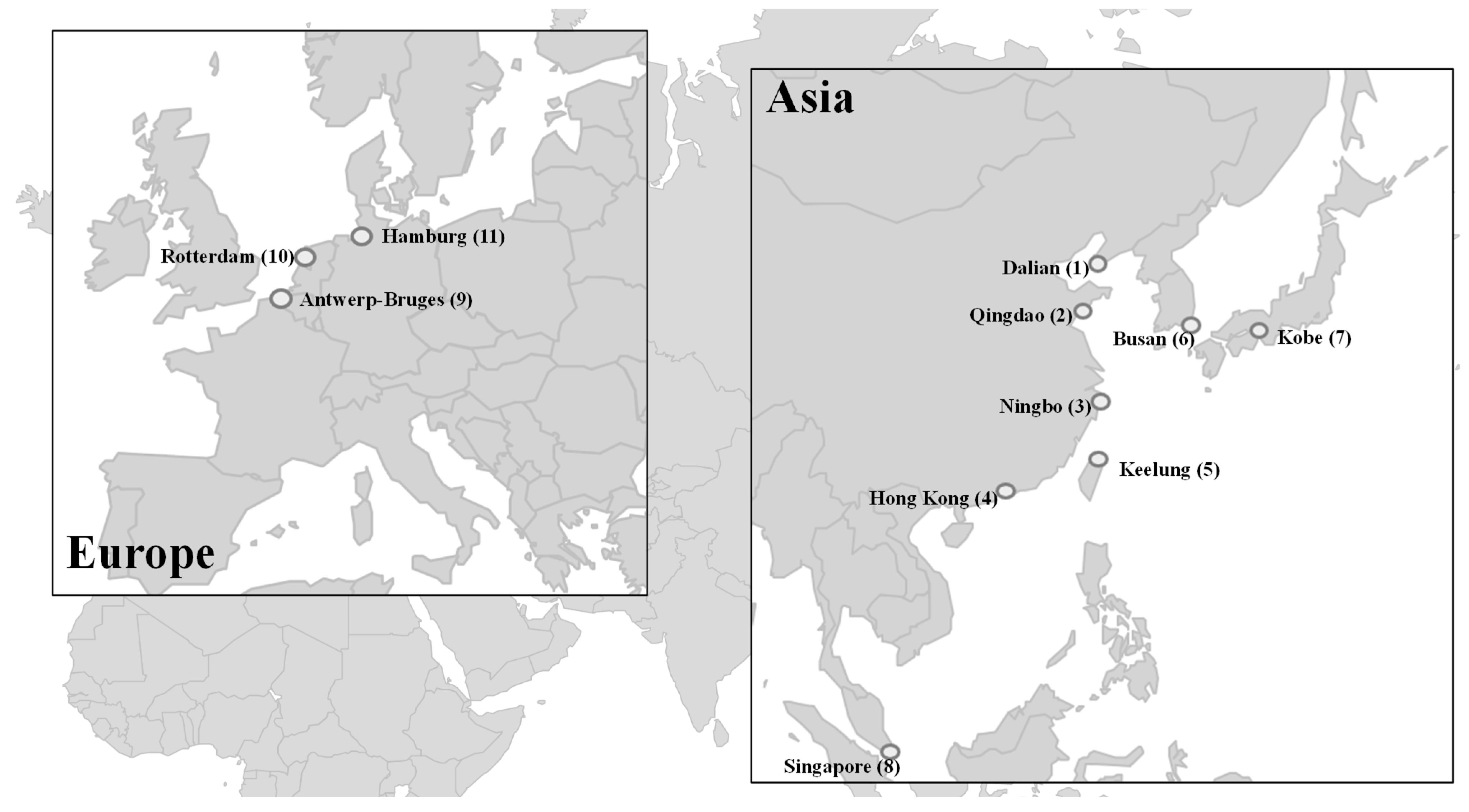
In terms of port parameter settings, we select 11 major ports as alternative ports of call, which include 8 Asian ports (i.e., Dalian, Qingdao, Ningbo, Hong Kong, Keelung, Busan, Kobe, and Singapore) and 3 European ports (i.e., Antwerp, Rotterdam, and Hamburg). The standard operating time for each port is set at 18 h [20]. The specific port information is detailed in

Table 2. Port information.

No.	Port Name	Port Code	Area
1	Port of Dalian	DAL	Asia
2	Port of Qingdao	QIN
3	Port of Ningbo	NBO
4	Port of Hong Kong	HKG
5	Port of Keelung	KEE
6	Port of Busan	BUS
7	Port of Kobe	KOB
8	Port of Singapore	SGP
9	Port of Antwerp-Bruges	ANT	Europe
10	Port of Rotterdam	ROT
11	Port of Hamburg	HAM

, and the locations of the ports are shown in Figure 5. With respect to liner characteristic analysis, we focus on two mainstream liner classes: 16,000 TEU and 20,000 TEU. The selection of these two liner classes is based on two considerations: first, these two liner classes represent the primary liners currently used in long-distance liner shipping; second, they allow for comparative analysis to explore the impact of the liner class on fuel selection. For each liner class, standard fuel consumption parameters are obtained from data provided by Clarksons Research, with adjustments made for different fuel types. For example, for the 16,000 TEU liner class, the fuel consumption parameters when VLSFO and methanol fuel are used require adjustments by factors of 1.6080 and 3.4490, respectively. Similarly, the adjustment factors for the 20,000 TEU liner class are 1.8280 and 3.9230. Detailed parameters can be found in

Table 3. Parameters of different liner classes.

Liner Class	Fuel Tank Capacity (×104 mt)	Fixed Cost (×104 USD/Week)	${\mathit{\alpha }}_{\mathbf{Methanol}}$	${\mathit{\alpha }}_{\mathbf{VLSFO}}$	${\mathit{v}}_{\mathbf{max}}$ (kn)	${\mathit{v}}_{\mathbf{min}}$ (kn)
16,000 TEU	0.8	57.4	0.0386	0.0180	15.0	26.0
20,000 TEU	1.0	60.9	0.0439	0.0205

.

In terms of fuel parameter settings, three types of fuel are considered: VLSFO, gray methanol, and green methanol. These fuels exhibit significant differences in energy density, carbon content, and price. The energy density of VLSFO is 40.2 MJ/kg, with a carbon content of 86%; in contrast, the energy density of methanol (both gray and green) is only 19.9 MJ/kg. With respect to carbon emissions, the combustion of 1 mt of VLSFO and gray methanol produces 3.16 mt and 1.38 mt of CO₂, respectively, whereas green methanol has carbon emissions that are close to zero. There are also notable price differences between the Asian and European markets, with specific parameters presented in

Table 4. Fuel prices at different ports (USD/mt).

Fuel Type	Port
	DAL	QIN	NBO	HKG	KEE	BUS	KOB	SGP	ANT	ROT	HAM
VLSFO	629	635	639	612	613	626	685	604	552	549	572
Gray methanol	338	341	345	353	351	345	348	359	350	339	339
Green methanol	696	699	703	702	709	704	707	714	699	697	697

. Fuel price data are derived from the available data published by Ship & Bunker.

Carbon tax parameters are based on global carbon tax data provided by the World Bank Carbon Pricing Dashboard. Taking regional differences into account, the carbon tax level in Asia is set to between 10 and 30 USD/mt of CO₂, whereas in Europe it is set to between 50 and 100 USD/mt of CO₂. Additionally, to ensure the convergence and computational efficiency of the algorithm, the population size of the genetic algorithm is set to 200, with a maximum number of iterations of 200, and the crossover and mutation rates are set at 0.9 and 0.1, respectively. For more information about the algorithm, see Gao, Xin, Li, Liu, and Chen [20], Chen, Yi, Xin, and Zhang [1] and Xiang, Xin, Zhang, Chen, and Liu [21].

6.1.2. Experimental Design

(1)

Experimental scheme design

In the following sections, we design a series of experiments to validate the effectiveness of the proposed model and algorithm and comprehensively analyze the impact of various factors on the LSSD for methanol-powered vessels. First, concerning the influence of fuel type, we investigate the performance of three types of fuel—VLSFO, gray methanol, and green methanol—when applied to two liner classes (e.g., 16,000 TEU liners and 20,000 TEU liners). The price of green methanol is set at 50% of the benchmark (i.e., set as 50% of the data given in Section 6.1.1), and relevant tax policies are fully implemented (i.e., set as 100% of the data given in Section 6.1.1). These experiments aim to analyze the impact of the large-scale production and widespread adoption of green methanol on LSSDs. Second, given that the cost of green methanol remains high due to production processes and limited economies of scale, we further examine the impact of the change in the price of green methanol on the LSSD. Two schemes are considered: one featuring the current price of green methanol and another with a 25% price reduction. By comparing bunkering strategies, speed management, and profitability under these schemes, we evaluate how price reductions in green methanol could facilitate shipping network design and how fuel price changes influence the decision-making of liner companies.

(2)

Computational environment and solution process

All the numerical experiments in this study are conducted on a workstation equipped with an Intel Core i7 12,700 K processor (3.6 GHz) and 32 GB of RAM, Santa Clara, CA, USA, running Windows 11 Professional. The algorithm was implemented in Python 3.8, with Gurobi 9.5 used as the optimization solver. The solution process is detailed as follows: each experimental scheme was independently run 30 times via different random seeds. The optimal solution and corresponding objective function value are recorded for each run, along with convergence curves, to evaluate the algorithm’s performance. The average computation time for each scheme was approximately 45 min, and the total computation time for all the schemes was approximately 120 h. The final results analyzed are the best solutions obtained through multiple runs.

6.2. Sensitivity Analysis

6.2.1. Sensitivity Analysis of Fuel Type

This section assumes that methanol is already widely used and conducts experiments to compare the impact of different fuels on liner companies’ profits. It is assumed that liner companies utilize VLSFO, gray methanol, and green methanol as liner fuels, forming three liner fleet operational schemes, designated as the VLSFO scheme, the gray methanol scheme, and the green methanol scheme, respectively.

As shown in Figure 6, the computational results in this section reveal a noteworthy phenomenon: under the current carbon tax policy framework, the VLSFO scheme and green methanol scheme demonstrate highly consistent optimization outcomes in terms of LSSD, whereas gray methanol shows significant disadvantages. Specifically, for 16,000 TEU liners, the green methanol scheme yields a revenue of USD 15.89 million, nearly identical to the USD 15.88 million from the VLSFO scheme, whereas the gray methanol scheme lags behind at only USD 14.82 million. A similar pattern emerges for 20,000 TEU liners, where the green methanol scheme generates a revenue of USD 19.42 million, which is slightly higher than the USD 19.23 million of the VLSFO scheme, whereas the revenue of gray methanol remains significantly lower at USD 18.54 million. This revenue disparity directly reflects the competitive viability of different fuel schemes in operational contexts. The fundamental cause of these differences lies in the interplay between fuel characteristics and policy factors. While methanol fuel’s energy density (i.e., 19.9 MJ/kg) is approximately half that of VLSFO (i.e., 40.2 MJ/kg), resulting in nearly double the fuel consumption, the expected 50% price reduction seen for green methanol combined with the carbon tax makes its overall cost comparable to that of the VLSFO scheme. In contrast, the gray methanol scheme bears both higher purchase costs and carbon tax expenses, which significantly undermines its economic competitiveness. Particularly when accounting for carbon tax costs, the total cost of the gray methanol scheme is substantially higher than those of the other two schemes, directly influencing shipping network design and operational strategy choices.

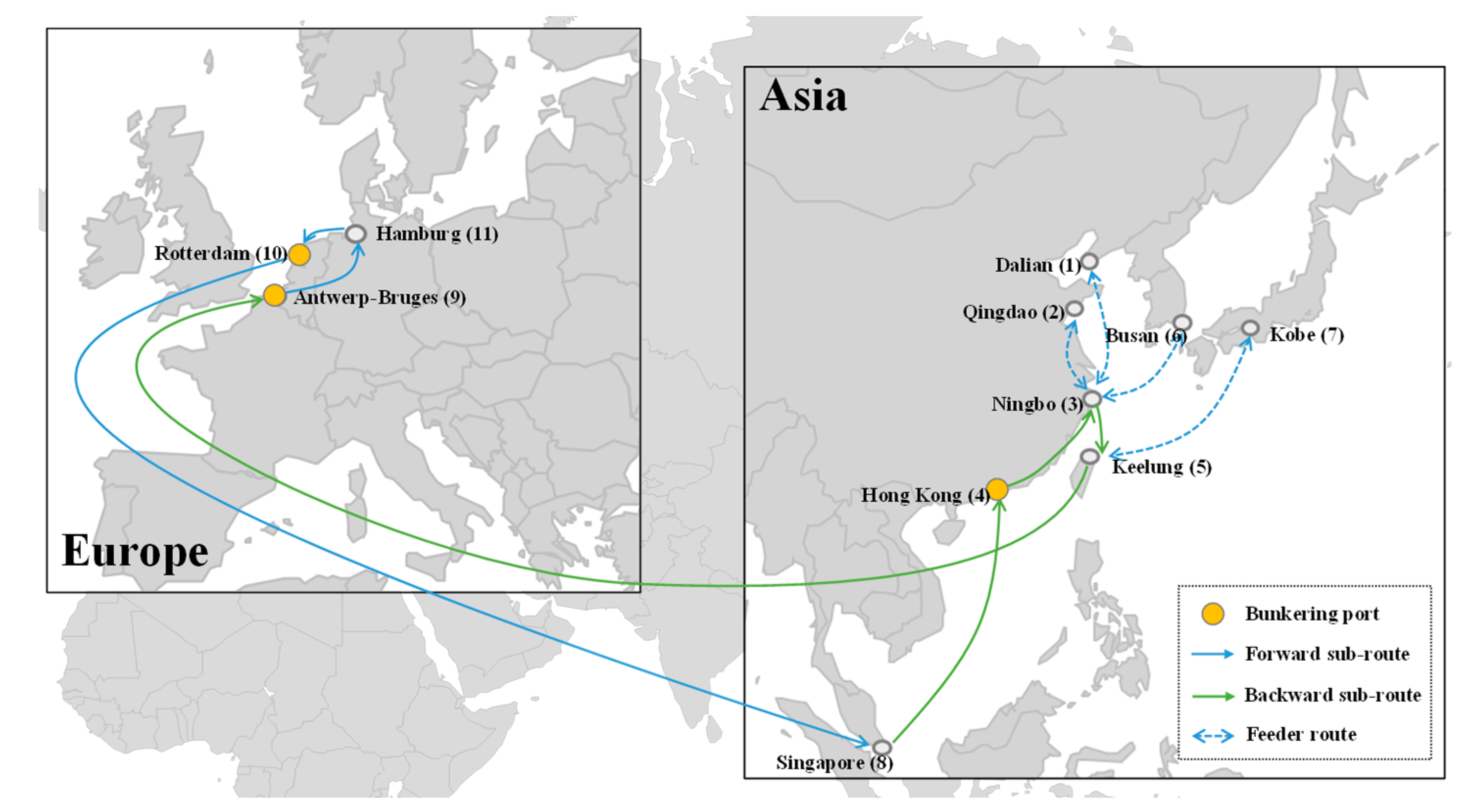
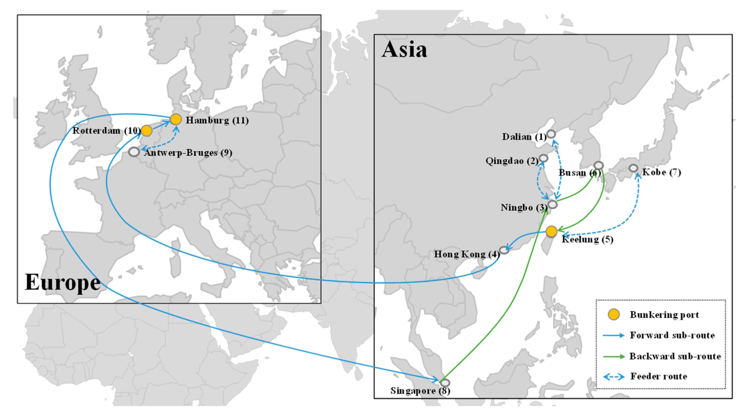
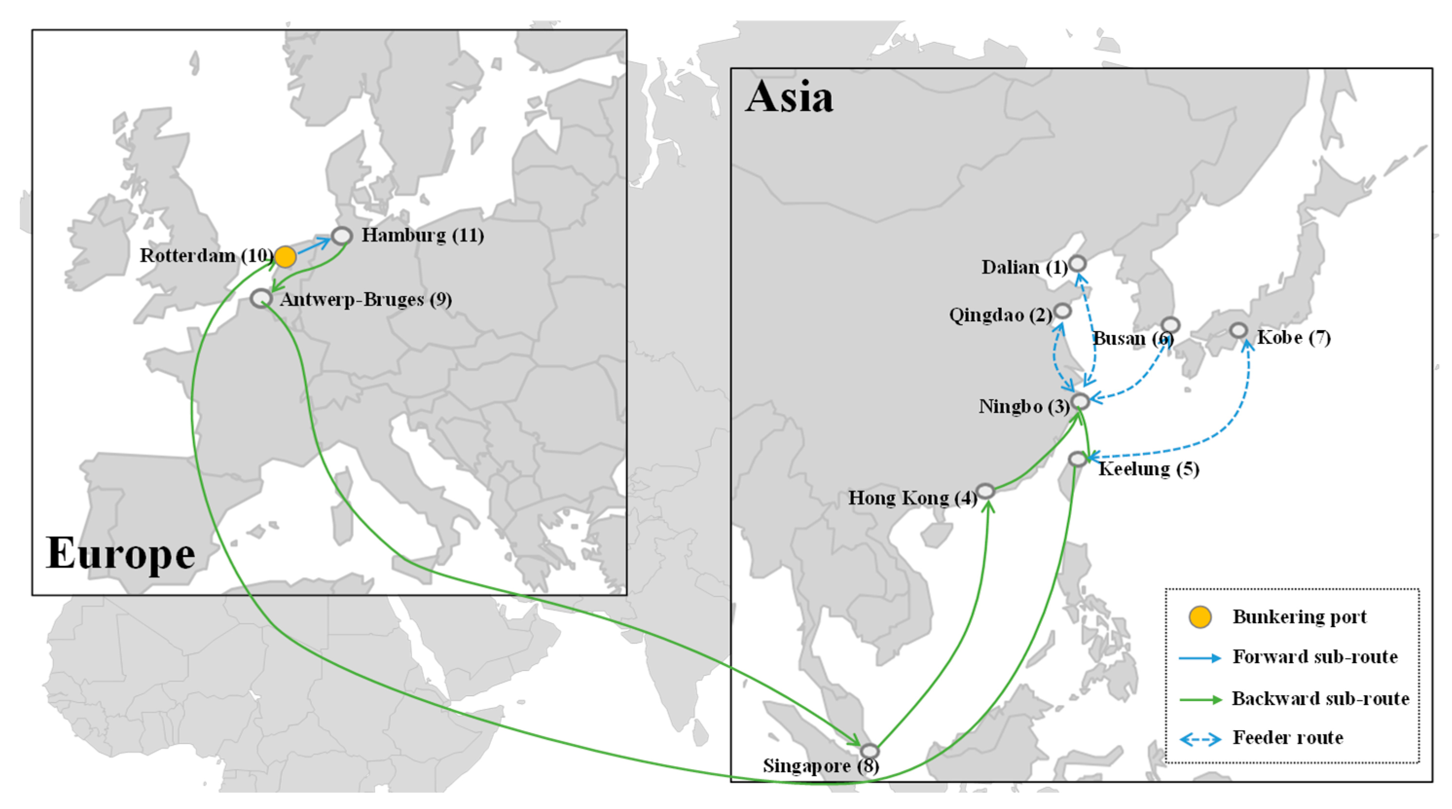
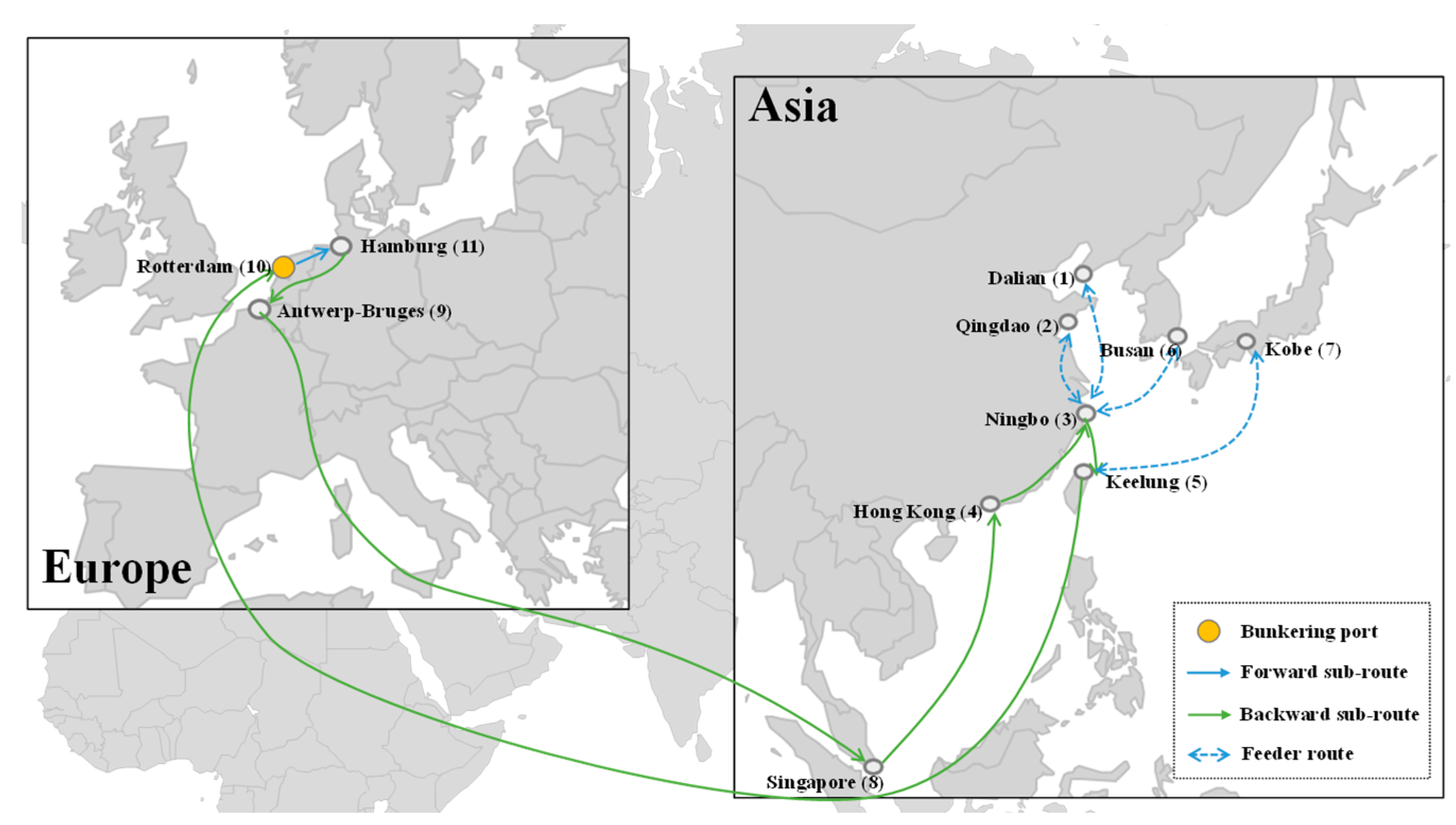
From the perspective of shipping network design, the disparate costs associated with the three schemes result in the manifestation of distinct characteristics, as illustrated in

Table 5. Shipping network structure with different fuel types.

Liner Class	Fuel Type	Trunk Route	Feeder Routes	Weekly Revenue (×106 USD)
16,000 TEU	Green methanol	ANT → HAM → ROT → SGP → HKG → NBO → KEE → ANT	DAL + QIN + BUS $\leftrightarrow$ NBO KOB $\leftrightarrow$ KEE	15.89
	Gray methanol	KEE → HKG → ROT → HAM → SGP → NBO → BUS → KEE	DAL + QIN $\leftrightarrow$ NBO KOB $\leftrightarrow$ KEE ANT $\leftrightarrow$ HAM	14.82
	VLSFO	ROT → HAM → ANT → SGP → HKG → NBO → KEE → ROT	DAL + QIN + BUS $\leftrightarrow$ NBO KOB $\leftrightarrow$ KEE	15.88
20,000 TEU	Green methanol	NBO → KEE → ROT → HAM → ANT → SGP → HKG → NBO	DAL + QIN + BUS $\leftrightarrow$ NBO KOB $\leftrightarrow$ KEE	19.42
	Gray methanol	NBO → KEE → HKG → ANT → ROT → HAM → SGP → NBO	DAL + QIN + BUS $\leftrightarrow$ NBO KOB $\leftrightarrow$ KEE	18.54
	VLSFO	NBO → BUS → KEE → HKG → ROT → HAM → ANT → SGP → NBO	DAL + QIN $\leftrightarrow$ NBO KOB $\leftrightarrow$ KEE	19.23

Note: In the table, the bold text represents the endpoint ports for the forward sub-routes, which also serve as the origin ports for the backward sub-routes. In the feeder routes, the symbol “+” indicates an “and” relationship. For example, DAL + QIN $\leftrightarrow$ NBO indicates that both DAL and QIN are feeder ports to the NBO.

and Figure 7, Figure 8, Figure 9, Figure 10, Figure 11 and Figure 12. For 16,000 TEU liners, the VLSFO scheme adopts the network structure ROT → HAM → ANT → SGP → HKG → NBO → KEE → ROT, characterized by a high degree of regional concentration in Europe. ROT, HAM, and ANT are situated in close proximity to one another, with ROT located 334 nautical miles from HAM and 411 nautical miles from ANT. Additionally, these locations offer comparable VLSFO pricing rates, with rates of USD 549, 572, and 552 per mt, respectively. The green methanol scheme follows a network structure of ANT → HAM → ROT → SGP → HKG → NBO → KEE → ANT, visiting the same European ports but rearranging the sequence to optimize bunkering strategies (green methanol prices at ANT, HAM, and ROT are USD 699, 697, and 697 per mt, respectively). Both schemes exhibit similar selection in terms of ports of call in the Asian area, choosing the SGP as the transshipment hub for Asia–Europe container transportation. This is due to the moderate fuel prices (USD 604 per mt for VLSFO and USD 714 per mt for green methanol) and the strategic geographical location of the SGP. In contrast, the gray methanol scheme reveals notable alterations in the shipping network’s structure. The selection of KEE as the port of call is indicative of its lower gray methanol price (USD 351 per mt). In the European region, the liner company reduces the number of ports of calls, with a round–trip arrangement between ROT and HAM that takes advantage of the lowest gray methanol prices (USD 339 per mt at both ports). These differences in the shipping network structure demonstrate the adjustments that are required in response to the higher cost pressures in the gray methanol scheme.

With respect to sailing speed management, the differences in cost structure also have a significant effect, as shown in

Table 6. Sailing speed management and bunker fuel management strategies.

Line Class	Fuel Type	Bunkering Amount (×104 mt)	Bunkering Ports	Number of Liners	Average Sailing Speed (kn)	Fuel Cost (×106 USD)
16,000 TEU	Green methanol	10.42	ANT, ROT, HKG	9	15.34	36.50
	Gray methanol	11.73	KEE, ROT, HAM	9	16.77	40.33
	VLSFO	4.93	ROT	9	15.25	27.07
20,000 TEU	Green methanol	12.16	NBO, ROT, HAM	9	16.23	42.53
	Gray methanol	11.66	NBO, ROT	9	15.46	39.91
	VLSFO	6.53	NBO, KEE, HKG, ROT	9	16.27	38.03

. For 16,000 TEU liners, the average speeds for the VLSFO and green methanol schemes are 15.25 knots and 15.34 knots, respectively, with a minimal difference of only 0.6%. This consistency directly reflects the similar cost pressures faced by the two schemes. For 20,000 TEU liners, the impact of cost structure differences is more pronounced. The average sailing speeds for the VLSFO and green methanol schemes remain consistent, whereas the average sailing speed for the gray methanol scheme decreases to 15.46 knots. This difference indicates that large liners, when subjected to high-cost pressures, are more inclined to reduce sailing speed as a strategy to control fuel consumption.

With respect to bunker fuel management strategies, differences in cost structure lead to distinct bunkering patterns. For 20,000 TEU liners, owing to variations in energy density, the total bunkering amount of green methanol reaches 121,600 mts, which is 86.22% greater than the 65,300 mts required for VLSFO. This difference aligns almost perfectly with the energy density ratio of two types of fuel (40.2 MJ/kg for VLSFO versus 19.9 MJ/kg for methanol), validating the theoretical expectations regarding the relationship between fuel consumption and energy density. In contrast, the bunkering amount for gray methanol is 116,600 mts, which is slightly lower than that for green methanol. This discrepancy is likely reflective of a more conservative bunker fuel management strategy, driven by the higher costs associated with specific legs. A more noteworthy aspect lies in the selection of bunkering ports. Under the VLSFO scheme, bunkering is conducted at NBO, KEE, HKG, and ROT, where the VLSFO prices are USD 639 per mt, USD 613 per mt, USD 612 per mt, and USD 549 per mt, respectively. In particular, ROT emerges as the primary bunkering port because it has the lowest fuel price, highlighting the sensitivity of traditional bunkering strategies to cost factors. For the green methanol scheme, bunkering is mainly carried out at NBO, ROT, and HAM. Although the green methanol prices at these ports are relatively high (at USD 703 per mt and USD 697 per mt), the overall cost remains competitive because of the balancing effect of carbon taxes. This pattern is further validated by the case of a 16,000 TEU vessel. The bunkering amount under the VLSFO scheme is 49,300 mt, whereas the bunkering volumes under the green methanol and gray methanol schemes are 104,200 mt and 117,300 mt, respectively.

By comparing the three schemes in terms of shipping network design, sailing speed management, and bunkering fuel management strategies, a critical system feature emerges: the carbon tax framework creates a unique equilibrium. The green methanol scheme (with higher fuel consumption but no carbon tax) and the VLSFO scheme (with lower fuel prices but a carbon tax) achieve comparable overall cost levels, resulting in similar optimization outcomes. This balance is evident, not only in total profit but also in terms of specific operational decisions, such as similar shipping network designs, comparable speed management, and bunkering fuel management strategies.

6.2.2. Sensitivity Analysis of Fuel Price

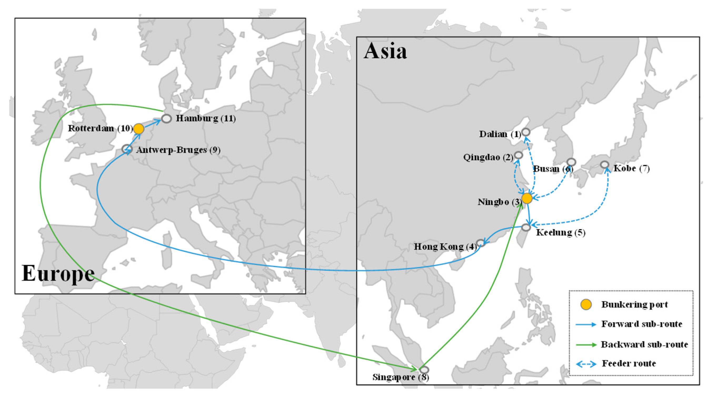
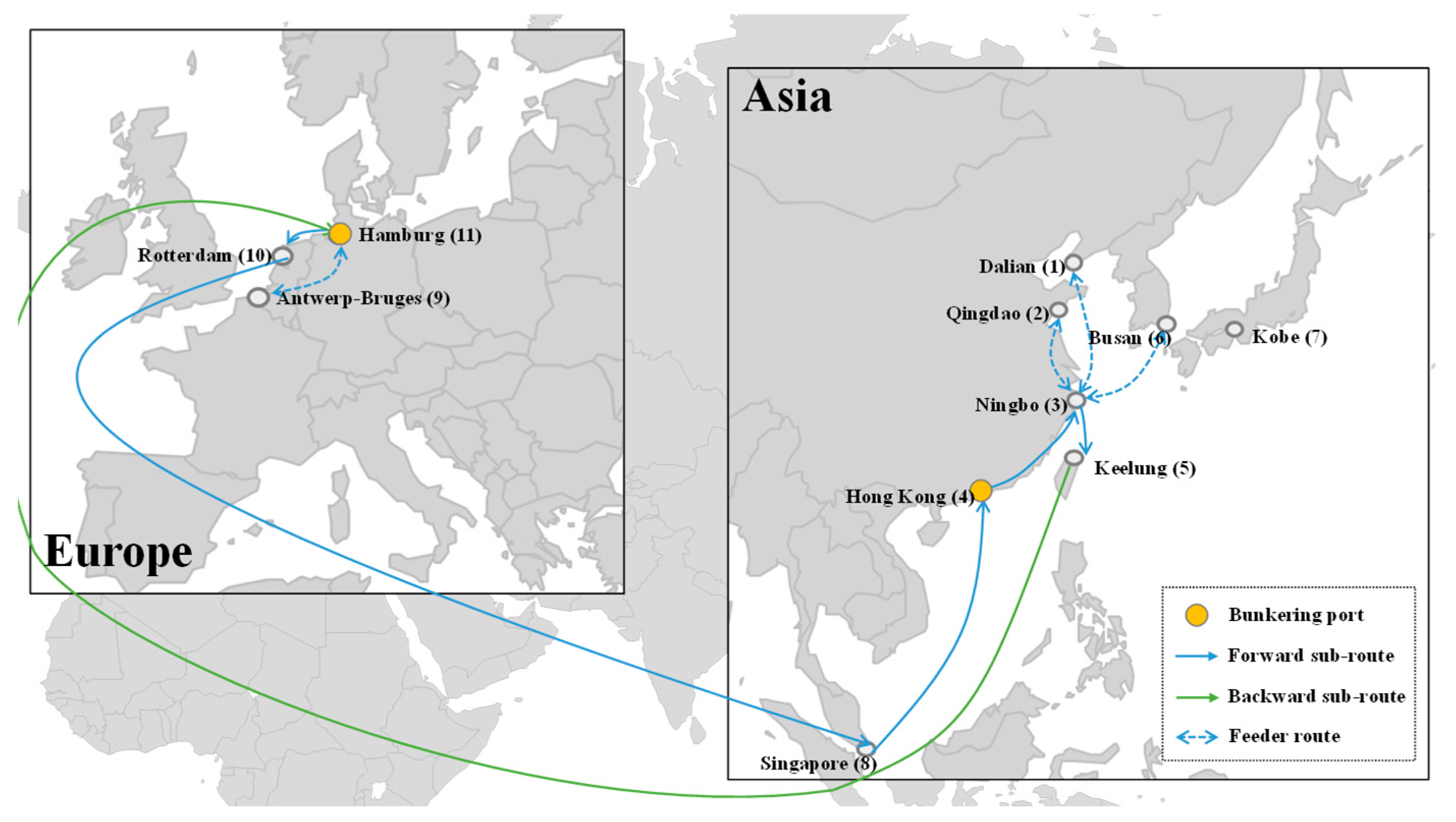
The current high price of green methanol is largely due to production capacity limitations and the fact that the product is in the early stage of supply chain development. In this section, we analyze the impact of price changes under two scenarios: the current price level and a 25% price reduction. The experimental results indicate that price changes trigger comprehensive adjustments in LSSD. In terms of the shipping network design scheme, price levels primarily influence network complexity and the selection of hub ports, as shown in

Table 7. Shipping network structure with 100% price level of green methanol.

Fuel Type	Liner Class	Trunk Route	Feeder Routes	Weekly Revenue (×106 USD)
Green methanol	16,000 TEU	HAM → ROT → SGP → HKG → NBO → KEE → HAM	DAL + QIN + BUS $\leftrightarrow$ NBO ANT $\leftrightarrow$ HAM	11.74
	20,000 TEU	ANT → ROT → SGP → HKG → KEE → NBO → HKG → ANT	DAL + QIN + BUS $\leftrightarrow$ NBO KOB $\leftrightarrow$ KEE HAM $\leftrightarrow$ ROT	14.17

Note: In the table, the bold text represents the endpoint ports for the forward sub-routes, which also serve as the origin ports for the backward sub-routes. In the feeder routes, the symbol “+” indicates an “and” relationship. For example, DAL + QIN + BUS NBO indicates that DAL, QIN, and BUS are feeder ports to the hub port NBO.

and Figure 13 and Figure 14. Under the current price level, the network for 16,000 TEU liners tends to be simplified, with the truck route HAM → ROT → SGP → HKG → NBO → KEE → HAM comprising only six hub ports and showing clear regional concentration. The European leg (HAM → ROT) and the Asian leg (HKG → NBO → KEE) form independent regional clusters, connected via the SGP as a transshipment hub port. After a 25% price reduction, the shipping network expands to NBO → KEE → HKG → ANT → ROT → HAM → SGP → NBO, with ANT added as a new hub port. This demonstrates that lower fuel costs enable the liner company to expand its shipping network and select more hub ports, thereby improving profitability. For 20,000 TEU liners, the network changes from ANT → ROT → SGP → HKG → KEE → NBO → HKG → ANT to NBO → QIN → KEE → HKG → ANT → ROT → SGP → NBO. In the shipping network under the current price level, HKG is called at twice, but in the network under the 25% price reduction scenario HKG is called at only once and QIN is added as a hub port. The network structure adjustment serves to underscore the strategic importance of green methanol for northern Chinese ports. As a critical port connecting Northeast Asia, the geographic advantage of the QIN allows it to cover the vast northern container transportation market while providing efficient green methanol bunkering services through its advanced infrastructure, positioning it as an important hub for supporting green shipping development.

Moreover, liner shipping network expansion directly impacts liner operational strategies, particularly liner sailing speed management. The results in

Table 8. Sailing speed management and bunker fuel management strategies with 100% price of green methanol.

Fuel Type	Liner Class	Bunkering Amount (×104 mt)	Bunkering Ports	Number of Liners	Average Speed (kn)	Fuel Cost (×106 USD)
Green methanol	16,000 TEU	10.06	HAM, HKG	9	15.16	70.25
	20,000 TEU	10.89	ANT, ROT, HKG	9	15.25	76.03

show that the average speed of both liner classes increases from 15.16 knots to 15.36 knots for 16,000 TEU liners and from 15.25 knots to 15.41 knots for 20,000 TEU liners. Particularly on long-haul legs (e.g., leg ROT-SGP), the liner sailing speed changes are more pronounced. For 20,000 TEU liners, the speed on this leg increases from 15.01 knots to 16.10 knots, whereas for 16,000 TEU liners, the increase is more moderate, from 15.01 knots to 15.72 knots. These differences reflect the trade-offs in operational strategies: larger liners prioritize speed to enhance service quality, whereas medium-classed liners focus on balanced shipping network coverage.

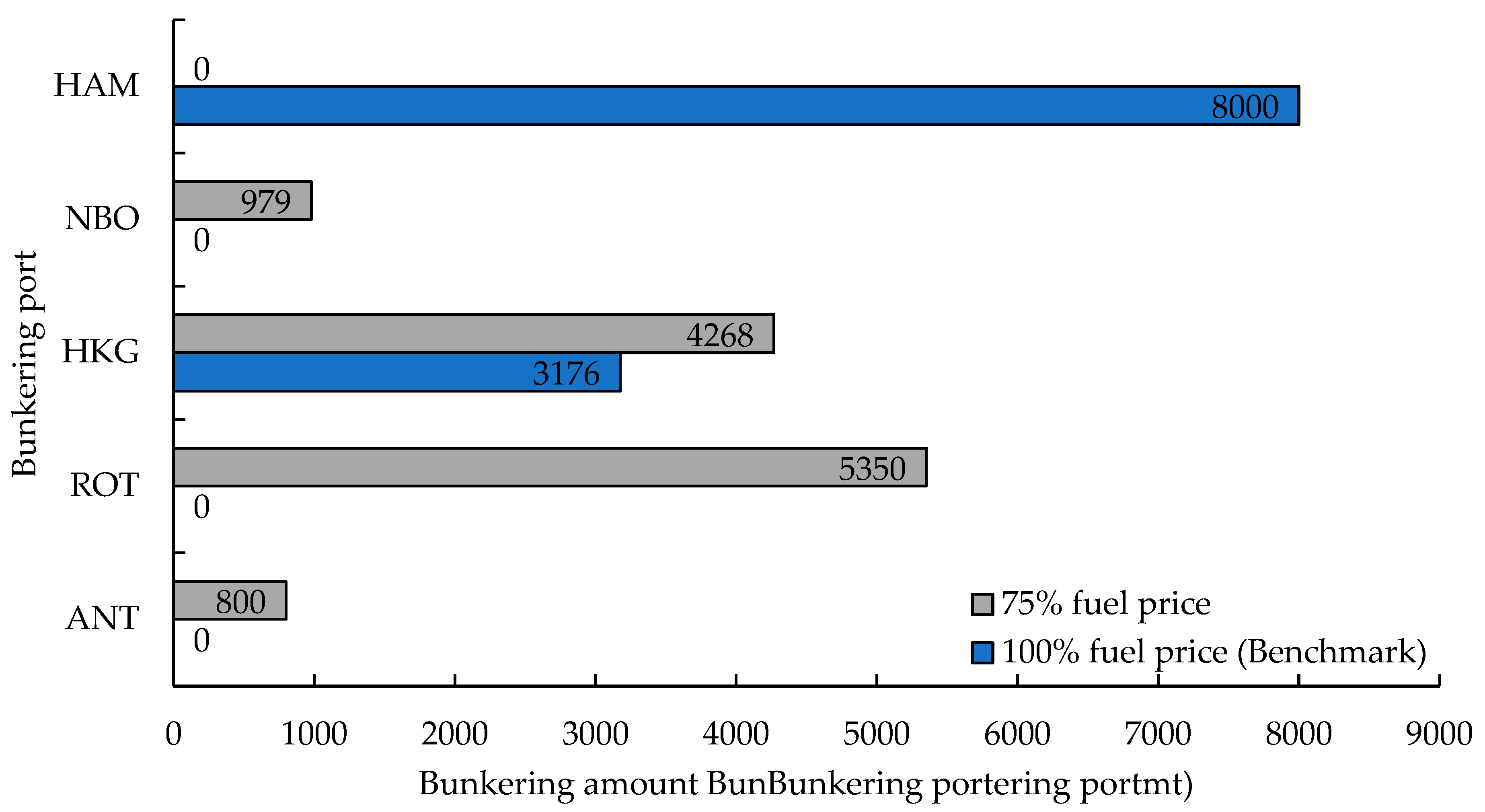
Bunker fuel management strategies also undergo fundamental adjustments with fuel price changes. Under the current price level, bunkering is highly concentrated at European ports, accounting for more than 70% of the total bunkering amount (e.g., for 16,000 TEU liners, 71% of the total bunkering amount occurs at HAM). The concentration is attributable to the relatively low fuel price of HAM, which is USD 697/mt, in comparison with the price of USD 714/mt at SGP and USD 699/mt at ANT. Following a reduction in fuel price, bunker fuel management strategies shift to a multiport distributed bunkering model (as illustrated in Figure 15), with the emergence of new bunkering ports (i.e., NBO, ANT, and ROT), while HAM is removed. Furthermore, the amount of fuel bunking at HKG increased from 3176 mt to 4268 mt, representing a 34.38% increase. For 20,000 TEU liners, under the current price level, more than 75% of the bunkering amount occurs at ROT. Following a reduction in fuel price, the proportions of bunkering amount are adjusted to 44% ROT, 48% QIN, and 8% NBO, thereby creating a more balanced bunkering network. The emergence of the QIN as a bunkering port likely benefits from its strategic location, which facilitates the coverage of the Asian container transportation network. This adjustment also serves to illustrate the growing role of Asian ports in the global green shipping system and offers valuable insights for Asian bunkering ports. As green fuels become more prevalent, it is imperative that the QIN and other Asian ports enhance their fuel supply capabilities to attract a greater bunkering demand. Furthermore, the emergence of a multiport distributed bunkering model indicates that regional collaboration and competition among ports will intensify. Securing a dominant position in the green fuel supply chain and becoming the preferred choice for global liner companies will be pivotal to future development.

In terms of fuel consumption, price reductions have different impacts. The weekly fuel consumption for the 16,000 TEU and 20,000 TEU liners increases from 10.06 mts and 10.89 mts to 10.26 mts and 11.98 mts, respectively. These changes are ultimately reflected in economic performance: for 16,000 TEU liners, fuel costs decrease by 23.40% (i.e., from USD 70.25 million to USD 53.81 million). For 20,000 TEU liners, costs decline by 17.44% (i.e., from USD 76.03 million to USD 62.77 million). Considering various costs, the total weekly profit for 16,000 TEU liners increases from USD 11.74 million to USD 13.91 million (an increase of 18.48%), and for 20,000 TEU liners, it increases from USD 14.17 million to USD 16.12 million (an increase of 13.76%). Notably, although the percentage increase in revenue for 20,000 TEU liners is smaller, their absolute revenue advantage remains, indicating that larger liners retain an economic edge, even under reduced green methanol prices.

Overall, the decline in green methanol prices triggers coordinated optimization across multiple elements in LSSD. Network expansion creates opportunities for adjustments in sailing speed management and bunker fuel management strategies, whereas improved operational efficiency supports more flexible shipping network patterns, ultimately forming a virtuous cycle. The two liner classes demonstrate disparate adaptation strategies throughout this process. For the 20,000 TEU liner class, the liner company concentrates on leveraging economies of scale and enhancing operational efficiency to maximize profits, whereas for the 16,000 TEU liners class, the company prioritizes expanding market coverage to increase revenue. This systemic transformation indicates that as green methanol production technology advances and economies of scale are achieved, the shipping industry is positioned to accelerate its transition toward sustainable development while maintaining economic feasibility.

7. Conclusions

In this paper, we investigate the liner shipping system design (LSSD) for methanol-powered vessels in the context of the green fuel transformation currently underway in the shipping industry. By constructing a bi-level programming model, key decision-making aspects such as shipping network design, liner speed management, and bunker fuel management strategies (i.e., bunkering port selection and bunkering amount determination) are integrated with traditional network design decisions (i.e., fleet deployment, shipping network design and slot allocation). Considering the nonlinear terms in the model (e.g., the fuel consumption function), we propose a model reformulation method based on a piecewise linearization approach. Then, considering the NP-hard properties of the problem, we develop an algorithm based on the framework of the genetic algorithm (GA) to solve the model. Moreover, we conduct sensitivity analyses for fuel types (i.e., HFO, gray methanol, and green methanol) and fuel prices. The calculation results for different experimental scenarios are used to capture managerial insights to support the green fuel transition for liner companies. Moreover, the experimental results can also provide the necessary decision support for governments and regional and international organizations to formulate scientific policies for carbon reduction and fuel transition in the shipping industry. Based on experimental analyses using real-world shipping data, we derive a series of conclusions:

• In the comparative analysis of fuel types, we find that the optimization results for green methanol-powered liners and VLSFO-powered liners are highly consistent under the current carbon tax framework, whereas gray methanol-powered liners have significant disadvantages. This finding has important policy implications. On the one hand, the current carbon tax mechanism successfully achieves its policy goals by making green fuels and traditional fuels equally competitive in actual operation through economic means. On the other hand, the double cost pressure caused by higher fuel costs and a carbon tax may prompt the shipping industry to transition directly from traditional fuels to green fuels, bypassing gray methanol as a transitional stage. In addition, these results provide critical insights into the decarbonization pathway for the shipping industry; that is, the design of policy tools can directly influence technological choices.
• Fuel price levels significantly impact the trade-offs that liner companies make between shipping network complexity and operational efficiency. Under the current price level, the network for 16,000 TEU liners covers only six hub ports. When the price of green methanol decreases by 25%, the number of hub ports expands to seven. Moreover, bunker fuel management strategies shift from a high concentration (with the main ports accounting for 75% of the total bunkering amount) to a more distributed model (with the main ports accounting for only 44%). This result indicates that fuel price reductions can encourage liner companies to increase competitiveness through network expansion rather than by focusing solely on cost control.
• We find a significant interaction between liner class and green transition strategies. The liners of different classes respond differently to price changes. For example, 20,000 TEU liners demonstrate a stronger potential for operational efficiency improvement after fuel price reductions, with weekly profit increasing from USD 14.17 million to USD 16.12 million (a 13.76% increase). In contrast, 16,000 TEU liners exhibit greater flexibility in shipping network optimization, with weekly profit increasing from USD 11.74 million to USD 13.91 million (an 18.48% increase). This is driven by network expansion to increase market coverage. This difference suggests that sensitivity to green fuel subsidies varies by liner class and that green transition policies should be tailored to liner classes to maximize policy effectiveness.
• Bunker fuel management strategies shift from a high-concentration model to a more distributed model. With fuel price reductions, bunker fuel management strategies exhibit decentralized characteristics, reflecting a dynamic trade-off between operational flexibility and cost control for liner companies. For example, the 16,000 TEU liners shifted from a concentrated bunkering strategy at HAM to bunkering at both ANT and ROT, whereas the 20,000 TEU liners added QIN as a bunkering hub. Decision-makers at the QIN and other Asian ports should invest in infrastructure to support the development of green fuel bunkering capabilities.

Overall, this is the first paper that considers a bunker fuel management strategy in LSSD. We hope that by discussing this emerging issue, we can extend the existing container liner shipping network design model. Notably, this paper still has several limitations, and the following directions can be considered for future research. First, we can explore how combinations of different fuels affect shipping network design. Currently, liner companies can choose to bunker different types of fuel for liners in different regions to meet policy requirements. In the above context, the liner shipping network design problem is undoubtedly practical and complex. Second, fuel price fluctuations are a typical uncertainty that liner companies must address. Therefore, discussing our problem in the context of considering this uncertainty would also be an interesting research direction.

References

1. Chen, K.; Yi, X.; Xin, X.; Zhang, T. Liner shipping network design model with carbon tax, seasonal freight rate fluctuations and empty container relocation. Sustain. Horiz. 2023, 8, 100073. [Google Scholar] [CrossRef]
2. Shangguan, Y.; Tian, X.; Pang, K.-W.; Ruan, Q.; Jin, Y.; Wang, S. Navigating the green shipping: Stochastic hydrogen hub deployment in inland waterways. Transp. Res. Part D Transp. Environ. 2024, 129, 104126. [Google Scholar] [CrossRef]
3. Tian, X.; Shangguan, Y.; Pang, K.-W.; Guo, Y.; Lyu, M.; Wang, S.; Huang, G.Q. Carbon emission allocation policy making in liner shipping: A novel approach toward equitable and efficient maritime sustainability. Ocean Coast. Manag. 2024, 256, 107270. [Google Scholar] [CrossRef]
4. Yang, W.; Chen, X.; Liu, Y. Review and reflections of legislation and policies on shipping decarbonization under China’s “dual carbon” target. Front. Mar. Sci. 2023, 10, 1131552. [Google Scholar] [CrossRef]
5. Hu, Z.; Huang, Y.; Sun, L.; Qi, X.; Pan, X. Study on international carbon emission quota allocation of shipping industry-based on fairness and efficiency. Front. Mar. Sci. 2023, 10, 1269643. [Google Scholar] [CrossRef]
6. Christiansen, M.; Hellsten, E.; Pisinger, D.; Sacramento, D.; Vilhelmsen, C. Liner shipping network design. Eur. J. Oper. Res. 2020, 286, 1–20. [Google Scholar] [CrossRef]
7. Wang, S.; Meng, Q. Container liner fleet deployment: A systematic overview. Transp. Res. Part C Emerg. Technol. 2017, 77, 389–404. [Google Scholar] [CrossRef]
8. Karsten, C.V.; Brouer, B.D.; Pisinger, D. Competitive liner shipping network design. Comput. Oper. Res. 2017, 87, 125–136. [Google Scholar] [CrossRef]
9. Ting, S.-C.; Tzeng, G.-H. An optimal containership slot allocation for liner shipping revenue management. Marit. Policy Manag. 2004, 31, 199–211. [Google Scholar] [CrossRef]
10. Shintani, K.; Imai, A.; Nishimura, E.; Papadimitriou, S. The container shipping network design problem with empty container repositioning. Transp. Res. Part E Logist. Transp. Rev. 2007, 43, 39–59. [Google Scholar] [CrossRef]
11. Ronen, D. Cargo ships routing and scheduling: Survey of models and problems. Eur. J. Oper. Res. 1983, 12, 119–126. [Google Scholar] [CrossRef]
12. Lane, D.; Heaver, T.D.; Uyeno, D. Planning and scheduling for efficiency in liner shipping. Marit. Policy Manag. 1987, 14, 109–125. [Google Scholar]
13. Rana, K.; Vickson, R.G. A model and solution algorithm for optimal routing of a time-chartered containership. Transp. Sci. 1988, 22, 83–95. [Google Scholar]
14. Ronen, D. Ship scheduling: The last decade. Eur. J. Oper. Res. 1993, 71, 325–333. [Google Scholar]
15. Dulebenets, M.A.; Pasha, J.; Abioye, O.F.; Kavoosi, M. Vessel scheduling in liner shipping: A critical literature review and future research needs. Flex. Serv. Manuf. J. 2021, 33, 43–106. [Google Scholar]
16. Chen, J.; Ye, J.; Zhuang, C.; Qin, Q.; Shu, Y. Liner shipping alliance management: Overview and future research directions. Ocean Coast. Manag. 2022, 219, 106039. [Google Scholar]
17. Elmi, Z.; Singh, P.; Meriga, V.K.; Goniewicz, K.; Borowska-Stefańska, M.; Wiśniewski, S.; Dulebenets, M.A. Uncertainties in liner shipping and ship schedule recovery: A state-of-the-art review. J. Mar. Sci. Eng. 2022, 10, 563. [Google Scholar] [CrossRef]
18. Meng, Q.; Wang, S. Optimal operating strategy for a long-haul liner service route. Eur. J. Oper. Res. 2011, 215, 105–114. [Google Scholar] [CrossRef]
19. Meng, Q.; Wang, S. Liner shipping service network design with empty container repositioning. Transp. Res. Part E Logist. Transp. Rev. 2011, 47, 695–708. [Google Scholar]
20. Gao, S.; Xin, X.; Li, C.; Liu, Y.; Chen, K. Container ocean shipping network design considering carbon tax and choice inertia of cargo owners. Ocean Coast. Manag. 2022, 216, 105986. [Google Scholar]
21. Xiang, Z.; Xin, X.; Zhang, T.; Chen, K.; Liu, M. Asia–Europe liner shipping network design model considering Arctic route and black carbon tax. Ocean Coast. Manag. 2025, 261, 107492. [Google Scholar] [CrossRef]
22. Agarwal, R.; Ergun, Ö. Network design and allocation mechanisms for carrier alliances in liner shipping. Oper. Res. 2010, 58, 1726–1742. [Google Scholar] [CrossRef]
23. Arslan, O.; Archetti, C.; Jabali, O.; Laporte, G.; Speranza, M.G. Minimum cost network design in strategic alliances. Omega 2020, 96, 102079. [Google Scholar] [CrossRef]
24. Besbes, O.; Savin, S. Going bunkers: The joint route selection and refueling problem. Manuf. Serv. Oper. Manag. 2009, 11, 694–711. [Google Scholar]
25. Vilhelmsen, C.; Lusby, R.; Larsen, J. Tramp ship routing and scheduling with integrated bunker optimization. EURO J. Transp. Logist. 2014, 3, 143–175. [Google Scholar] [CrossRef]
26. He, P.; Jin, J.G.; Pan, W.; Chen, J. Route, speed, and bunkering optimization for LNG-fueled tramp ship with alternative bunkering ports. Ocean Eng. 2024, 305, 117957. [Google Scholar] [CrossRef]
27. Omholt-Jensen, S.; Fagerholt, K.; Meisel, F. Fleet repositioning in the tramp ship routing and scheduling problem with bunker optimization: A matheuristic solution approach. Eur. J. Oper. Res. 2025, 321, 88–106. [Google Scholar] [CrossRef]
28. Yao, Z.; Ng, S.H.; Lee, L.H. A study on bunker fuel management for the shipping liner services. Comput. Oper. Res. 2012, 39, 1160–1172. [Google Scholar] [CrossRef]
29. Kim, H.-J.; Chang, Y.-T.; Kim, K.-T.; Kim, H.-J. An epsilon-optimal algorithm considering greenhouse gas emissions for the management of a ship’s bunker fuel. Transp. Res. Part D Transp. Environ. 2012, 17, 97–103. [Google Scholar]
30. Kim, H. A Lagrangian heuristic for determining the speed and bunkering port of a ship. J. Oper. Res. Soc. 2014, 65, 747–754. [Google Scholar]
31. Sheng, X.; Lee, L.H.; Chew, E.P. Dynamic determination of vessel speed and selection of bunkering ports for liner shipping under stochastic environment. OR Spectr. 2014, 36, 455–480. [Google Scholar]
32. Meng, Q.; Wang, S.; Lee, C.-Y. A tailored branch-and-price approach for a joint tramp ship routing and bunkering problem. Transp. Res. Part B: Methodol. 2015, 72, 1–19. [Google Scholar]
33. Zhen, L.; Wang, S.; Zhuge, D. Dynamic programming for optimal ship refueling decision. Transp. Res. Part E Logist. Transp. Rev. 2017, 100, 63–74. [Google Scholar]
34. Aydin, N.; Lee, H.; Mansouri, S.A. Speed optimization and bunkering in liner shipping in the presence of uncertain service times and time windows at ports. Eur. J. Oper. Res. 2017, 259, 143–154. [Google Scholar]
35. De, A.; Choudhary, A.; Turkay, M.; Tiwari, M.K. Bunkering policies for a fuel bunker management problem for liner shipping networks. Eur. J. Oper. Res. 2021, 289, 927–939. [Google Scholar]
36. Wang, H.; Liu, Y.; Wang, S.; Zhen, L. Optimal Ship Deployment and Sailing Speed under Alternative Fuels. J. Mar. Sci. Eng. 2023, 11, 1809. [Google Scholar] [CrossRef]
37. Svanberg, M.; Ellis, J.; Lundgren, J.; Landälv, I. Renewable methanol as a fuel for the shipping industry. Renew. Sustain. Energy Rev. 2018, 94, 1217–1228. [Google Scholar]
38. Parris, D.; Spinthiropoulos, K.; Ragazou, K.; Giovou, A.; Tsanaktsidis, C. Methanol, a Plugin Marine Fuel for Green House Gas Reduction—A Review. Energies 2024, 17, 605. [Google Scholar] [CrossRef]
39. Gao, T.; Tian, J.; Liu, C.; Huang, C.; Wu, H.; Yuan, Z. A model for speed and fuel refueling strategy of methanol dual-fuel liners with emission control areas. Transp. Policy 2025, 161, 1–16. [Google Scholar]
40. Chen, K.; Lu, Q.; Xin, X.; Yang, Z.; Zhu, L.; Xu, Q. Optimization of empty container allocation for inland freight stations considering stochastic demand. Ocean Coast. Manag. 2022, 230, 106366. [Google Scholar]
41. Li, Z.; Wang, L.; Wang, G.; Xin, X.; Chen, K.; Zhang, T. Investment and subsidy strategy for low-carbon port operation with blockchain adoption. Ocean Coast. Manag. 2024, 248, 106966. [Google Scholar]
42. De, A.; Wang, J.; Tiwari, M.K. Fuel bunker management strategies within sustainable container shipping operation considering disruption and recovery policies. IEEE Trans. Eng. Manag. 2019, 68, 1089–1111. [Google Scholar]
Figure 1. A toy shipping network.
Jmse 13 00709 g001
Figure 2. A schematic diagram of the LSSD.
Jmse 13 00709 g002
Figure 3. The overall framework of the algorithm.
Jmse 13 00709 g003
Figure 4. A schematic diagram of coding and decoding.
Jmse 13 00709 g004
Figure 5. Port location (with their numbers in brackets).
Jmse 13 00709 g005
Figure 6. Effects of different fuel types on profit, fuel cost, and average sailing speed.
Jmse 13 00709 g006
Figure 7. Shipping network structure with 16,000 TEU green methanol-powered liners.
Jmse 13 00709 g007
Figure 8. Shipping network structure with 16,000 TEU gray methanol-powered liners.
Jmse 13 00709 g008
Figure 9. Shipping network structure with 16,000 TEU VLSFO-powered liners.
Jmse 13 00709 g009
Figure 10. Shipping network structure with 20,000 TEU green methanol-powered liners.
Jmse 13 00709 g010
Figure 11. Shipping network structure with 20,000 TEU gray methanol-powered liners.
Jmse 13 00709 g011
Figure 12. Shipping network structure with 20,000 TEU VLSFO-powered liners.
Jmse 13 00709 g012
Figure 13. Shipping network structure with 16,000 TEU green methanol-powered liners (100% price level).
Jmse 13 00709 g013
Figure 14. Shipping network structure with 20,000 TEU green methanol-powered liners (100% price level).
Jmse 13 00709 g014
Figure 15. Influence of fuel price on bunkering amount (16,000 TEU green methanol-powered liner).
Jmse 13 00709 g015