Active Disturbance Rejection Control for DC Motor Laboratory Plant Learning Object ^†

Abstract

The paper deals with learning objects for introductory modeling of simple dynamical systems and design of controllers with disturbance observer-based integral action. They can be used to illustrate the design process of state controllers, state and disturbance observers, as well as to get in touch with a popular approach called active disturbance rejection control (ADRC). In both cases, external disturbances along with errors resulting from model inaccuracies are reconstructed using the extended state observer (ESO). In addition to simulation and design of regulators and observers in Matlab/Simulink, the learning objects focus on the development of relevant terminology and competencies in the field of simulation, modeling and experimentation in traditional laboratories, with the support of LMS Moodle and remote control. The main innovativeness of the paper is to clarify the relationship of ADRC to the traditional state space controllers design and modeling by using two types of linear models approximating controlled nonlinear systems.

1. Introduction

The state-space approach to the analysis and design of control systems has been developed in the 1960s. As a part of the “Modern Control Theory (MCT)”, it was supposed to eliminate all deficiencies of the traditional proportional–integral–derivative control, as, for example, the windup effect of the integral action appearing under constrained control. Under known plant input, the system’s state should be enough to predict future system behavior, which might be used for dealing with time delays in next steps. Effects of unknown disturbance could be taken into account by using appropriate disturbance models [1,2]. Its states then enlarged the state vector corresponding to the plant dynamics.

1.1. Model-Based versus Model-Free Approaches

Various results of the state space approach can now be found as part of an alternative known as active rejection control (ADRC). Based on the school by H.S. Tsien, the ADRC has been proposed by J. Han [3] and further developed by Z. Gao [4,5] and many co-workers. It is often applied in applications using complex nonlinear mechatronic systems (see, e.g., [6,7,8,9]). Some latest ADRC experimental results in energy systems are in [10,11], while other approaches can be found, e.g., in [12,13,14]. They see the PID control as a result of an empirical design made without a mathematical model. They find the root of theory vs. practical hassle in the established MCT and primal practices antagonism. Nevertheless, MCT does not have to rely on precise mathematical models. Its application to the solved problems can be impractical and inflexible, so that its internal abilities to deal with uncertainties are ignored. Some current papers are not precise when interpreting ADRC as a model-free approach, which is in contrast to the traditional model-based analysis and designs. Namely ADRC is also model-based, but uses simpler models, like integrating models. Some models are derived from complex and nonlinear systems, approximated by the zeroth therm of their Taylor series expansion around some (possibly variable) working point [15]. The locally “frozen” internal feedback of integrating models can then be combined with possible internal and external errors to produce equivalent disturbance in order to create an “ultra-local” plant model [16]. Such a simplification can be justified not only by engineering intuition, but also by mathematical tools. Simply, in Taylor’s expansion, only the zeroth term will be used instead of zeroth and the first term.

1.2. History Started Long Time Ago

ADRC and other postmodern “model-free” approaches based on integrating models (such as Model-Free Control—MFC, developed by M. Fliess and co-workers [16]) are often seen as “paradigm shifts”. Simplifications that can be easily explained by using two types of linear models can be traced back to the origins of control theory. Let us, for example, mention the famous controller tuning method by Ziegler and Nichols [17]. Their identification of step responses by a tangent drawn through the inflection point can also be interpreted as an approximation of plants by an integrating model of the device with a linearly increasing step response that is shifted by time delay. Feldbaum [18] in his book on optimal control, discusses the early patent of Russian engineers from 1935 using quadratic velocity feedback—a feature typical for minimum time control of double integrator systems. The implementation was much easier than the implementation of a minimal time control based on “usual” linear plant model. A similar approach was later developed by J. Han [3] in the ADRC.

1.3. Problem Statement and Contribution of the Paper

The goal of the learning objects designed for ADRC is:

• to present the reconstruction and compensation of the disturbances provided by this method as the simplest case of a more general approach to the reconstruction of an extended state vector including equivalent disturbance, which is then compensated for by an opposite signal, the state controller design and the delay compensation,
• to discuss several approaches in approximating nonlinear systems by linear models of different complexity,
• to explain relations between ADRC and MCT.

Next, it will be shown how these learning objects can be developed and used within the experiment-based learning framework. In order to highlight the differences between the conventional design in the state space and the ADRC, the coefficients a, which are usually used in linear first order plant models, are highlighted by red. Substitution $a=0$ in the equations corresponds to ADRC.

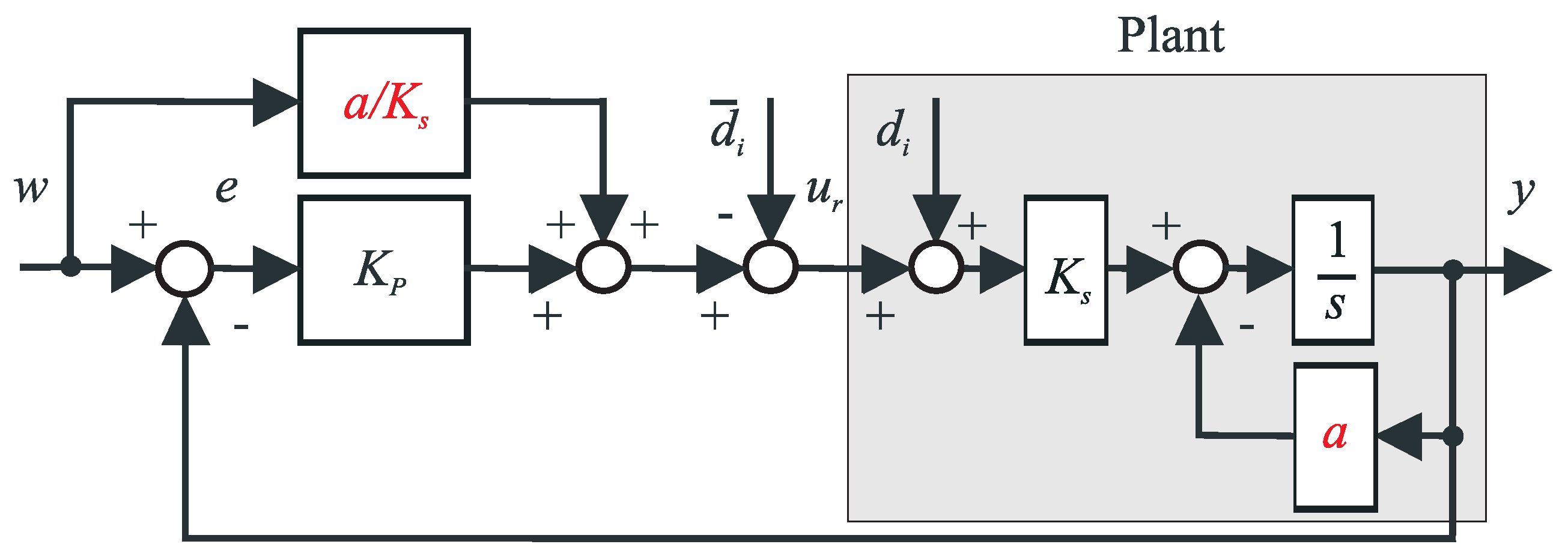
2. Compensation of Input Disturbances

2.1. Controller Derivation

For a piecewise constant setpoint value $w=const$ yielding the control error $e=w-y$, by using the plant model expressed in differential equation form:

$${\displaystyle \frac{dy}{dt}}=\dot{y}=K_s[u_r+d_i]-ay=-{\displaystyle \frac{de}{dt}}$$

(1)

while the required model for the control error dynamics equals

$$\dot{e}=\lambda e,$$

(2)

where for $\lambda <0$ the error decreases exponentially in time. The control signal $u_r$ is as follows:

$$u_r=K_P(w-y)+aw/K_s-d_i;K_P=-\left(\lambda +a\right)/K_s$$

(3)

Obviously, when based on a reconstructed $d_i=d+d_m$, the merging effect of an external disturbance d and of a modeling disturbance $d_m$ due to model uncertainty, should be counteracted at the P-controller output (Figure 1). It should be noted that for $a=0$ the modeling disturbance includes also the internal feedback which equals to $-ay$.

2.2. Reconstruction of an Input Disturbances by ESO

The model of equivalent disturbance $d_i$ represents a new state variable. A piece-wise constant $d_i$, e.g., step function, can correspond to a sequence of Dirac pulses at an integrator input (Figure 2), because each step function can be described by integral of Dirac delta function. The corresponding state-space plant model is therefore

$$\begin{array}{c}\dot{\mathbf{x}}=\left[\begin{array}{cc}-a& K_s\\ 0& 0\end{array}\right]\mathbf{x}+\left[\begin{array}{c}{K}_s\\ 0\end{array}\right]u+\left[\begin{array}{c}0\\ 1\end{array}\right]\delta \hfill \\ y=\left[\begin{array}{c}10\end{array}\right]\mathbf{x}\hfill \end{array}$$

(4)

where $\mathbf{x}=\left[\begin{array}{c}y\\ d_i\end{array}\right]$.

The extended state observer (ESO) contains correction of the state variables proportional to the difference between the plant and the model output y - $\overline{y}$ (weighted by $p_1$ and $p_2$): The unknown signal $\delta$ acting on plant in Figure 2 can not be directly measured. Therefore, it should be reconstructed by input and output tracking (see Figure 3):

$$\begin{array}{c}\dot{\overline{\mathbf{x}}}=\left[\begin{array}{cc}-a& K_s\\ 0& 0\end{array}\right]\overline{\mathbf{x}}+\left[\begin{array}{c}{K}_s\\ 0\end{array}\right]u+\left[\begin{array}{c}{p}_1\\ p_2\end{array}\right](y-\overline{y})\hfill \\ \overline{\mathbf{x}}=\left[\begin{array}{c}\overline{y}\\ {\overline{d}}_i\end{array}\right];\overline{y}=\left[\begin{array}{c}10\end{array}\right]\overline{\mathbf{x}}\hfill \end{array}$$

(5)

The piecewise constant disturbance $d_i$ may also be used for slowly varying input disturbances approximation. In more general cases, e.g., for linearly increasing or decreasing disturbances, or for periodic disturbances, the higher order disturbance models have to be used.

2.3. Observer Tuning

After substituting $\overline{y}=\left[10\right]\overline{\mathbf{x}}$ into the state equation in (5), we get extended state-observer as a system with inputs consisting of the plant output $\left(y\right)$ and input $\left(u\right)$ signals:

$$\begin{array}{c}\dot{\overline{\mathbf{x}}}=\left[\begin{array}{cc}-p_1-a& K_s\\ -p_2& 0\end{array}\right]\overline{\mathbf{x}}+\left[\begin{array}{c}{K}_s\\ 0\end{array}\right]u+\left[\begin{array}{c}{p}_1\\ p_2\end{array}\right]y\hfill \\ \overline{\mathbf{x}}=\left[\begin{array}{c}\overline{y}\\ {\overline{d}}_i\end{array}\right];\overline{y}=\left[\begin{array}{c}10\end{array}\right]\overline{\mathbf{x}}\hfill \end{array}$$

(6)

Observer’s state matrix

$$\begin{array}{c}{\mathbf{A}}_s=s\mathbf{I}-\mathbf{A}=\left[\begin{array}{cc}s+p_1+a& -K_s\\ p_2& s\end{array}\right];\hfill \end{array}$$

(7)

has the following characteristic polynomial:

$$A_s\left(s\right)=s^2+\left(p_1+a\right)s+p_2{K}_s={(s-\lambda )}^2=s^2-2\lambda s+{\lambda }^2$$

(8)

By choosing a double pole $\lambda <0$, which may represent the only tuning parameter, we get the observer gains

$$p_1=-2\lambda -a;p_2={\lambda }^2/K_s$$

(9)

Frequently, the time constant $T_c=-1/\lambda$ is used instead of pole $\lambda$.

3. Real Experiments

In paper [19], we have demonstrated two experiments by a fan speed (RPM) control. In this paper we expand the experiments section by presenting the results on a DC motor. The laboratory DC motor plant model is shown in Figure 4.

The plant is based on Arduino UNO micro controller, the angular velocity (system output) of the DC motor is measured by optical encoder. The adjustment screw on the left side of the plant can provide additional load. In this paper it is controlled via Matlab Simulink environment using Serial communication at 115,200 baud. The sampling frequency is 100 Hz. The control signal from Matlab/Simulink is an integer in the range of 0–255, which is used by arduino controller to make pulse width modulated (PWM) signal with duty cycle in range of 0–100% proportionally. The PWM signal frequency is 980 Hz.

3.1. Step Response-Based Plant Approximation

The process model parameters are calculated from step response. The DC motor input range is 0 to 6 V. The chosen working point is 3 V, since the plant static input-output characteristics is the most linear there, as can be seen from Figure 5. All the experiments were performed without any additional load.

In Figure 6 there are two step responses. The first corresponds to input step from 0 to 3 V, to bring the plant to the desired working point. The second response corresponds to input step change from 3 V to 4 V. The process parameters are calculated from the second step-response.

The plant dynamics, approximated by static first-order transfer function:

$$\begin{array}{c}\hfill G_s\left(s\right)=\frac{K_s}{s+a}=\frac{2371.1}{s+1.031}\end{array}$$

(10)

is in Figure 7.

This model ensures good match between the model and the controlled system in chosen working point.

Simpler, the single integrator model approximation at the steepest part of the step response in Figure 8 yields

$$\begin{array}{c}\hfill G_s\left(s\right)=\frac{K_s}{s}=\frac{4237.5}{s}\end{array}$$

(11)

Such a model appears to be less accurate, but has better local fitting after step-change. As we shown later, the model (11) may be more suitable for controller design. When compared with the results from paper [19], obtained by a different laboratory model, $K_s$ of integrating model is now higher than the static model gain.

Remark 1.

As obvious from Figure 2, a more realistic plant approximation could be based on the first-order models with a dead-time $T_d$. After approximating its value by nth order time constant $T=T_d/n,n\ge 2$ range of appropriate controller gains may be estimated by the root-locus method. Range of applicable closed loop poles/time constants $T_c$ may then be determined according to (3).

The control loop in Figure 9 employs P controller with static feed-forward and extended state observer. Several combinations of closed-loop poles and models have been used for controller tuning. The controller gain $K_p$ from (3) can be tuned, e.g., by root locus method. The experiments performed on DC motor plant start from a steady-state at setpoint 3000 RPM, then a setpoint step change is made from 3000 RPM to 4000 RPM. After the process output is stabilized at 60 s, the input disturbance is applied by subtracting 0.5 V from the control signal. In Figure 10, Figure 11, Figure 12 and Figure 13 it can be seen, that the control signal does not reach the same steady-state value because of the heating produced by the previous experiments.

3.2. Qualitative and Quantitative Evaluation

When evaluating the control quality, the performance of the closed-loop response should be quantified. The speed of transients is usually quantified by Integrated Absolute Error (IAE) [20]. The shapes of optimal transients will be quantified by the deviation from a piece-wise monotonicity of the manipulated variable and process input variable in terms of a modified total variation TV (see, e.g., [21]). The results corresponding to all performed experiments are summarized in

Table 1. Performance measures—Setpoint step (SM: static model (10), IM: integrating model (11), ${\lambda }_1$: P controller closed loop pole, ${\lambda }_2$: observer pole).

$\mathit{Model}$	${\mathit{\lambda }}_1$	${\mathit{\lambda }}_2$	$\mathit{yIAE}$	${\mathit{uTV}}_1$	${\mathit{yTV}}_0$
SM	−2.5	−1	533.73	5.894491825	9428
IM	−2.5	−1	1833.07	6.043284497	9330
SM	−2.5	−2.5	562.56	6.432918939	9832
IM	−2.5	−2.5	1096.26	6.371039265	9840
SM	−2.5	−5	536.6	6.168313879	8808
IM	−2.5	−5	817.45	6.402538277	9968
SM	−4	−1	353.29	11.10806451	8852
IM	−4	−1	1284.97	9.749876336	9690
SM	−4	−4	581.09	13.99768388	10342
IM	−4	−4	635.88	9.301805688	9248
SM	−4	−5	481.41	9.220900011	6424
IM	−4	−5	565.48	5.201099543	4656
SM	−5	−3	405.22	11.52032935	6684
IM	−5	−3	576.62	6.499809124	4900
SM	−5	−5	564.62	19.41022646	10788
IM	−5	−5	483.33	12.97349199	10470
SM	−5	−7	558.19	27.23828	14294
IM	−5	−7	439.34	12.70464701	10124
SM	−1.5	−1.5	813.45	2.19723531	10444
IM	−1.5	−1.5	2331.15	3.8604877	9710
SM	−0.9	−1	1367.53	0.656394532	9516
IM	−0.9	−1	5150.8	1.888246085	8310

and

Table 2. Performance measures—Disturbance step (SM: static model (10), IM: integrating model (11), ${\lambda }_1$: P controller closed loop pole, ${\lambda }_2$: observer pole).

$\mathit{Model}$	${\mathit{\lambda }}_1$	${\mathit{\lambda }}_2$	$\mathit{yIAE}$	${\mathit{uTV}}_1$	${\mathit{yTV}}_0$
SM	−2.5	−1	1069	6.084217084	10264
IM	−2.5	−1	1684.36	6.001085686	10638
SM	−2.5	−2.5	528.65	6.046843664	10086
IM	−2.5	−2.5	765.64	6.30994367	10390
SM	−2.5	−5	308.09	5.555957642	9238
IM	−2.5	−5	482.41	6.428117495	11284
SM	−4	−1	661.9	10.74076305	8286
IM	−4	−1	1105.84	9.660718058	10492
SM	−4	−4	331.16	12.84074021	9874
IM	−4	−4	421.18	9.542247448	9682
SM	−4	−5	281.49	7.017225253	5284
IM	−4	−5	357.57	5.178514655	4922
SM	−5	−3	281.01	10.68852441	6496
IM	−5	−3	408.24	6.238420898	4870
SM	−5	−5	310.79	17.52628653	10348
IM	−5	−5	302.5	12.46486024	10322
SM	−5	−7	340.16	22.66275	12826
IM	−5	−7	253.18	10.90469989	8944
SM	−1.5	−1.5	1172.04	1.969434562	9856
IM	−1.5	−1.5	1940.44	3.283381832	10056
SM	−0.9	−1	2848.39	0.530924662	8474
IM	−0.9	−1	4608.22	1.920761782	10130

. Lower values correspond to better performance in all cases. Obviously, both models give comparable results (better in some cases, worse in others). Therefore, using a more complex model with $a\ne 0$ does not bring any significant improvements. However it can improve performance if suitable poles are chosen.

The transients corresponding to highlighted experiments in Table 1 and Table 2 are in Figure 10, Figure 11, Figure 12 and Figure 13.

4. Analysis of the Results

The evaluation of the first experiments opens the way to perform more complex experiments. In these experiments the students are supposed to relate the achieved performance with the plant step responses and their approximation, and to propose hypotheses regarding further performance improvements (see Remark 1).

4.1. Impact of the Tuning Parameter

Evaluation of the closed-loop pole selection (or its negative inverse—the time constant $T_c$) on the qualitative and quantitative properties of both control loops should give students enough data for making hypothesis regarding usefulness in practice and possible further modifications. When comparing the results from Table 1 and Table 2, the “static” model gives considerably better $yIAE$ values in cases where the closed-loop poles ${\lambda }_1>-5$ ($T_c>1/5$) for setpoint step change and disturbance step change, while keeping better total variances $uTV$ and $yTV$.

“Integrating” model gives better $yIAE$ performance in the majority of cases where the closed-loop poles ${\lambda }_1<-5$ ($T_c<1/5$), including better total variances $uTV$ and $yTV$. This corresponds to the highlighted section in Table 1 and Table 2.

The best value for each performance measure is highlighted by bold letters in Table 1 and Table 2.

It is worth mentioning, that the experiment yielding the best yIAE for disturbance step is obtained by using “integrating” model. On the other hand the closed-loop response with the same tuning, but employing the “static” model, yield the worst by far uTV and yTV performance (highlighted by italics letters).

Therefore, it seems right time to ask when to use the “static” model (which is mostly better and the difference is not so negligible as it seems) and when it may be more appropriate to use simpler integrating models. Students, along with identifying the boundaries of the proper use of both models, should design and discuss possible more complex modifications that should expand these boundaries and improve the control transients.

4.2. More Complex Controllers

As an obstacle to faster closed-loop dynamics by choosing lower $T_c$ values, students should find different delays of both models relative to the actual system. The discussion about delays can then lead to questions of an improved system approximations and to simple ways to balance the real plant and model dynamics (whereby the phase shift of the real plant reaction and the model is particularly clear in Figure 8). Several options can be identified:

• application of an additional time constant, or several shorter time constants [15] (see Remark 1), or
• application of a dead time.

These two alternatives can bring a number of solutions for further development including proportional–derivative (PD) and proportional–derivative–second derivative (PDD${}^2$) controller, straightforward plant dead time compensation by adding an equivalent delay to the ESO input from u, etc.

5. Alternative Disturbance Observer Design

While the state-space approach has advantages in its transparency, we quickly realized that the obtained results can be translated into polynomial form [22]. It is only necessary to derive the corresponding disturbance-to-output, or disturbance-to-input transfer functions.

5.1. ESO Expressed by Transfer Functions

The resulting ESO may be expressed by the transfer functions derived from

$$\begin{array}{c}{\mathbf{b}}_u=\left[\begin{array}{c}{K}_s\\ 0\end{array}\right];{\mathbf{b}}_y=\left[\begin{array}{c}{p}_1\\ p_2\end{array}\right];{\mathbf{c}}_d^t=\left[\begin{array}{c}01\end{array}\right]\hfill \\ S_{dy}={\displaystyle \frac{{\overline{D}}_i\left(s\right)}{Y\left(s\right)}}={\mathbf{c}}_d{\mathbf{A}}_s^{-1}{\mathbf{b}}_y={\displaystyle \frac{p_2\left(s+a\right)}{s^2+\left(p_1+a\right)s+p_2{K}_s}}\hfill \\ S_{du}={\displaystyle \frac{{\overline{D}}_i\left(s\right)}{U\left(s\right)}}={\mathbf{c}}_d{\mathbf{A}}_s^{-1}{\mathbf{b}}_u={\displaystyle \frac{-K_s{p}_2}{s^2+\left(p_1+a\right)s+p_2{K}_s}}\hfill \end{array}$$

(12)

After substitution for $p_2$ it can be seen, that the transfer function $S_{dy}$ contains inversion of the plant dynamics and chosen characteristic polynomial and the transfer function $S_{du}$ has a negative sign. The order of the characteristic polynomial is fixed by the sum of the plant model and the disturbance model orders to $n=2$ (see [19]).

5.2. ESO as a special case of Disturbance Observer (DOB)

The transfer-function-based Disturbance Observer (DOB) design has been firstly published by Ohishi and Ohnishi in 1987 [23,24]. The proposed solution considered the first order filters ($n=1$) in

$$\begin{array}{c}{S}_{dy}={\displaystyle \frac{{\overline{D}}_i\left(s\right)}{Y\left(s\right)}}={\displaystyle \frac{s+a}{K_s{(1+T_{f}s)}^n}}\hfill \\ S_{du}={\displaystyle \frac{{\overline{D}}_i\left(s\right)}{U\left(s\right)}}={\displaystyle \frac{-1}{{(1+T_{f}s)}^n}}\hfill \end{array}$$

(13)

Transfer function $S_{dy}$ includes inverse plant transfer function and a low-pass filter of the order $n\ge 1$. $S_{du}$ has a negative sign—the disturbance is reconstructed as difference of filtered actual plant input and filtered controller output. When choosing $n=2$ and $T_f=-1/{\lambda }_1$, we get results identical to (12). The use of higher-order filters can be advantageous in terms of improved noise attenuation [25]. As already mentioned, the design can be simplified by selecting $a=0$, as is common, for example, when designing speed controllers.

6. Discussion

In the comparisons above it was shown that there are no significant differences between transients corresponding to the controller based on the more detailed first-order (static) model (10) and the simple “ultra-local” integrating model (11). Although both solutions can be interpreted sufficiently well by the conventional state-space design, the second solution is now usually referred to as ADRC. While the differences between them appear to be negligible, they become larger when controlling second-order systems with constraints. So, for example, the ADRC solution for constrained systems presented in [3] offers significant simplifications, shorter execution times and significant increase of performance. Similar results in constrained, adaptive and possibly non-linear control, which are of particular importance in the automotive industry, have been presented few decades ago [26].

Today, similar design simplifications are not only used in ADRC and MFC [16], but also in other areas of control design, including, e.g., Generalized PID control with possibly higher-order derivatives [27] or solutions inspired by Smith’s predictor [28]. It seems that the “paradigm shift” in control design, based on two types of linear models, remains not only limited to these two isolated areas.

Together with the relevant textbooks and documents, this approach requires an extensive campaign supported by a wide range of experiments available.

7. Experimentation and Learning Aspects

The main goal of introducing extensive experiments into our control teaching is to increase the motivation of the students to deal with all the mathematical and theoretical tools required for a successful controller design of automotive systems. In this regard, our efforts seem to be well received by the students.

The approaches for reconstruction and compensation of disturbances can be combined with other alternatives, for example one or two degrees of freedom PI and IMC-PI controllers.

The students had to perform the following tasks from modeling:

(a)

measuring static input-output characteristic,

(b)

choosing working point in linear part of the static input to output characteristics,

(c)

measuring step response at the chosen working point,

(d)

calculating static first-order model parameters using measured step-response,

(e)

calculating integrating model parameters using measured step-response.

After obtaining both models, the control design and observer design tasks are as follows:

• implementing controllers,
• performing hands on real-time experiments using various combinations of closed-loop poles and disturbance observer gains,
• evaluating control quality using integral criteria, taking account the deviations from ideal shapes quantified by modified total variance criteria (see, e.g., [21]).

All of these tasks are performed by using real plant model described in Section 3. In this way, many other important related goals can be fulfilled as well, for example:

• manage, archive and save, process, visualize and present data that result from the extensive experiments,
• balance the individual development of required programs with pre-programmed tools,
• develop programming skills by the help of a control course,
• define certain program and data structures, etc.

One of the most serious problems we were facing significant differences in the speed of solving problems different students. A group of about 40 students was divided into two sub-groups working in pairs. One sub-group performs plant experiments, while the other develops simulations compared to the actual experiments. Sub-groups exchange tasks at a specific time. This work-flow requires strict synchronization. The problem can be partially alleviated by using remote experiments to finish the assignments. Nevertheless, with regard to security restrictions, this approach cannot be a generally acceptable solution. For teachers, the most difficult task (besides advising programming and control tasks) is to download, discuss, review and assess student assignments. We have already tested several approaches based on computer support [29], but a serious load still remains.

8. Conclusions

The paper presented core of the learning object, which compares the postmodern approach known as ADRC with the previous approach named “modern control”, which is based on an extended state observer. They differ in the ability to define two types of linear models—traditional “local” linear models based on the approximation of nonlinear feedback of the plant by the zeroth and the first terms of its Taylor expansion, while the new “model-free” approaches cover the “ultra-local” integrating linear models using only zeroth Taylor’s term. Although appearing in some papers and books from the early history of the control theory, e.g., in [17], the “model-free” approaches have not been given much attention for many decades. Increased opportunities for making experiments on real plants seem to change the “revolutionary paradigm” from the relatively isolated areas of ADRC and MFC to broader areas of control design.

References

1. Ackermann, J. Abtastregelung; Springer: Berlin, Germany, 1972. [Google Scholar]
2. Luenberger, D. Observers for multivariable systems. IEEE Trans. Autom. Control 1966, 11, 190–197. [Google Scholar] [CrossRef]
3. Han, J. From PID to Active Disturbance Rejection Control. Ind. Electron. IEEE Trans. 2009, 56, 900–906. [Google Scholar] [CrossRef]
4. Gao, Z. Active disturbance rejection control: A paradigm shift in feedback control system design. In Proceedings of the American Control Conference, Minneapolis, MN, USA, 14–16 June 2006; pp. 2399–2405. [Google Scholar]
5. Gao, Z. On the centrality of disturbance rejection in automatic control. ISA Trans. 2014, 53, 850–857. [Google Scholar] [CrossRef] [PubMed] [Green Version]
6. Hua, H.D.; Ma, N.; Ma, J.; Zhu, X.Y. Robust intelligent control design for marine diesel engine. J. Shanghai Jiaotong Univ. (Science) 2013, 18, 660–666. [Google Scholar] [CrossRef]
7. Pan, W.; Xiao, H.; Han, Y.; Wang, C.; Yang, G. Nonlinear active disturbance rejection controller research of main engine for ship. In Proceedings of the 2010 8th World Congress on Intelligent Control and Automation, Jinan, China, 7–9 July 2010; pp. 4978–4981. [Google Scholar]
8. Kang, E.; Hong, S.; Sunwoo, M. Idle speed controller based on active disturbance rejection control in diesel engines. Int. J. Automot. Technol. 2016, 17, 937–945. [Google Scholar] [CrossRef]
9. Wang, R.; Li, X.; Zhang, J.; Zhang, J.; Li, W.; Liu, Y.; Fu, W.; Ma, X. Speed Control for a Marine Diesel Engine Based on the Combined Linear-Nonlinear Active Disturbance Rejection Control. Math. Probl. Eng. 2018, 2018, 7641862. [Google Scholar] [CrossRef] [Green Version]
10. Sun, L.; Shen, J.; Hua, Q.; Lee, K.Y. Data-driven oxygen excess ratio control for proton exchange membrane fuel cell. Appl. Energy 2018, 231, 866–875. [Google Scholar] [CrossRef]
11. Sun, L.; Jin, Y.; You, F. Active disturbance rejection temperature control of open-cathode proton exchange membrane fuel cell. Appl. Energy 2020, 261, 114381. [Google Scholar] [CrossRef]
12. Parvathy, R.; Daniel, A.E. A survey on active disturbance rejection control. In Proceedings of the 2013 International Mutli-Conference on Automation, Computing, Communication, Control and Compressed Sensing (iMac4s), Kottayam, India, 22–23 March 2013; pp. 330–335. [Google Scholar]
13. Albertos, P.; Sanz, R.; Garcia, P. Disturbance rejection: A central issue in process control. In Proceedings of the 2015 4th International Conference on Systems and Control (ICSC), Sousse, Tunisia, 28–30 April 2015; pp. 1–8. [Google Scholar]
14. Zeng, G.Q.; Chen, J.; Chen, M.R.; Dai, Y.X.; Li, L.M.; Lu, K.D.; Zheng, C.W. Design of multivariable PID controllers using real coded population based extremal optimization. Neurocomputing 2015, 151, 1443–1453. [Google Scholar] [CrossRef]
15. Huba, M.; Oliveira, P.; Vrančič, D.; Bisták, P. ADRC as an Exercise for Modeling and Control Design in the State-Space. In Proceedings of the 6th-2019 International Conference on Control, Decision and Information Technologies, Paris, France, 23–26 April 2019. [Google Scholar]
16. Fliess, M.; Join, C. Model-free control. Int. J. Control 2013, 86, 2228–2252. [Google Scholar] [CrossRef] [Green Version]
17. Ziegler, J.G.; Nichols, N.B. Optimum settings for automatic controllers. Trans. ASME 1942, 64, 759–768. [Google Scholar] [CrossRef]
18. Feldbaum, A. Optimal Control Systems; Academic Press: New York, NY, USA, 1965. [Google Scholar]
19. Huba, M.; Hypiusová, M.; Tapák, P. Learning Objects and Experiments for Active Disturbance Rejection Control. In Proceedings of the 2019 5th Experiment International Conference (exp.at’19), Funchal, Madeira Island, Portugal, 12–14 June 2019; pp. 161–166. [Google Scholar]
20. Shinskey, F. How good are Our Controllers in Absolute Performance and Robustness. Meas. Control 1990, 23, 114–121. [Google Scholar] [CrossRef]
21. Huba, M. Performance measures, performance limits and optimal PI control for the IPDT plant. J. Process Control 2013, 23, 500–515. [Google Scholar] [CrossRef]
22. Huba, M.; Kul’ha, P. Saturating Control for the Dominant First Order Plants. In Proceedings of the IFAC Workshop “Motion Control”, Munich, Germany, 9–11 October 1995; pp. 197–204. [Google Scholar]
23. Ohishi, K. A new servo method in mechantronics. Trans. Jpn. Soc. Elect. Eng. 1987, 107-D, 83–86. [Google Scholar]
24. Ohishi, K.; Nakao, M.; Ohnishi, K.; Miyachi, K. Microprocessor-Controlled DC Motor for Load-Insensitive Position Servo System. IEEE Trans. Ind. Electron. 1987, IE-34, 44–49. [Google Scholar] [CrossRef]
25. Huba, M.; Bélai, I. Noise attenuation motivated controller design. Part I: Speed control. In Proceedings of the Speedam Symposium, Ischia, Italy, 18–20 June 2014; pp. 1325–1330. [Google Scholar]
26. Huba, M.; Sovišová, D.; Spurná, N. Digital Time-Optimal Control of Nonlinear Second-Order System. Prepr. 10th IFAC World Congr. 1987, 8, 29–34. [Google Scholar] [CrossRef]
27. Huba, M.; Vrančič, D. Comparing filtered PI, PID and PIDD2 control for the FOTD plants. In Proceedings of the 3rd IFAC Conference on Advances in Proportional-Integral-Derivative Control, Ghent, Belgium, 9–11 May 2018. [Google Scholar]
28. Huba, M.; Bélai, I. Limits of a Simplified Controller Design Based on IPDT models. ProcIMechE Part I J. Syst. Control Eng. 2018, 232, 728–741. [Google Scholar]
29. Ťapák, P. Real experiments marking in automatic control education. In Proceedings of the 2011 14th International Conference on Interactive Collaborative Learning, Piestany, Slovakia, 21–23 September 2011; pp. 281–284. [Google Scholar]
Figure 1. Controller design with compensation of an input disturbance d i = d + d m merging effect of an external disturbance d and of a modeling disturbance d m due to model uncertainty.
Information 11 00151 g001
Figure 2. Input disturbance d i may be interpreted as a new plant state of an integrator with a non-controlled and non-measurable input δ .
Information 11 00151 g002
Figure 3. Extended state observer design.
Information 11 00151 g003
Figure 4. DC motor laboratory plant.
Information 11 00151 g004
Figure 5. Static input-output characteristics.
Information 11 00151 g005
Figure 6. Process step-response.
Information 11 00151 g006
Figure 7. First order model approximation.
Information 11 00151 g007
Figure 8. Simple integrator model approximation.
Information 11 00151 g008
Figure 9. Closed control loop: P controller with static feed forward (orange), extended state observer (yellow), controlled plant (blue).
Information 11 00151 g009
Figure 10. Comparison—setpoint step—process variable.
Information 11 00151 g010
Figure 11. Comparison—disturbance step—process variable.
Information 11 00151 g011
Figure 12. Comparison—setpoint step—control signal.
Information 11 00151 g012
Figure 13. Comparison—disturbance step—control signal.
Information 11 00151 g013