Intensity of Bilateral Contacts in Social Network Analysis


Abstract
:1. Introduction
- explores the application of recent advances in SNA methods that allow the consideration of weights and direction in the calculation of clustering coefficients;
- proposes an approach to extract indicators that describe the behavioral aspects of the social network members; and
- develops a model that can explain the actors’ behavior through SNA indicators.
2. Related Work
- type of network analyzed;
- indicator type: Structural (conventional graph theory indicators), Activity (accounting for traffic, intensity or frequency of connections), or Clustering (local, “small world” indicators);
- use of direction in connections; and
- weights used (in the case of weighted indicators).
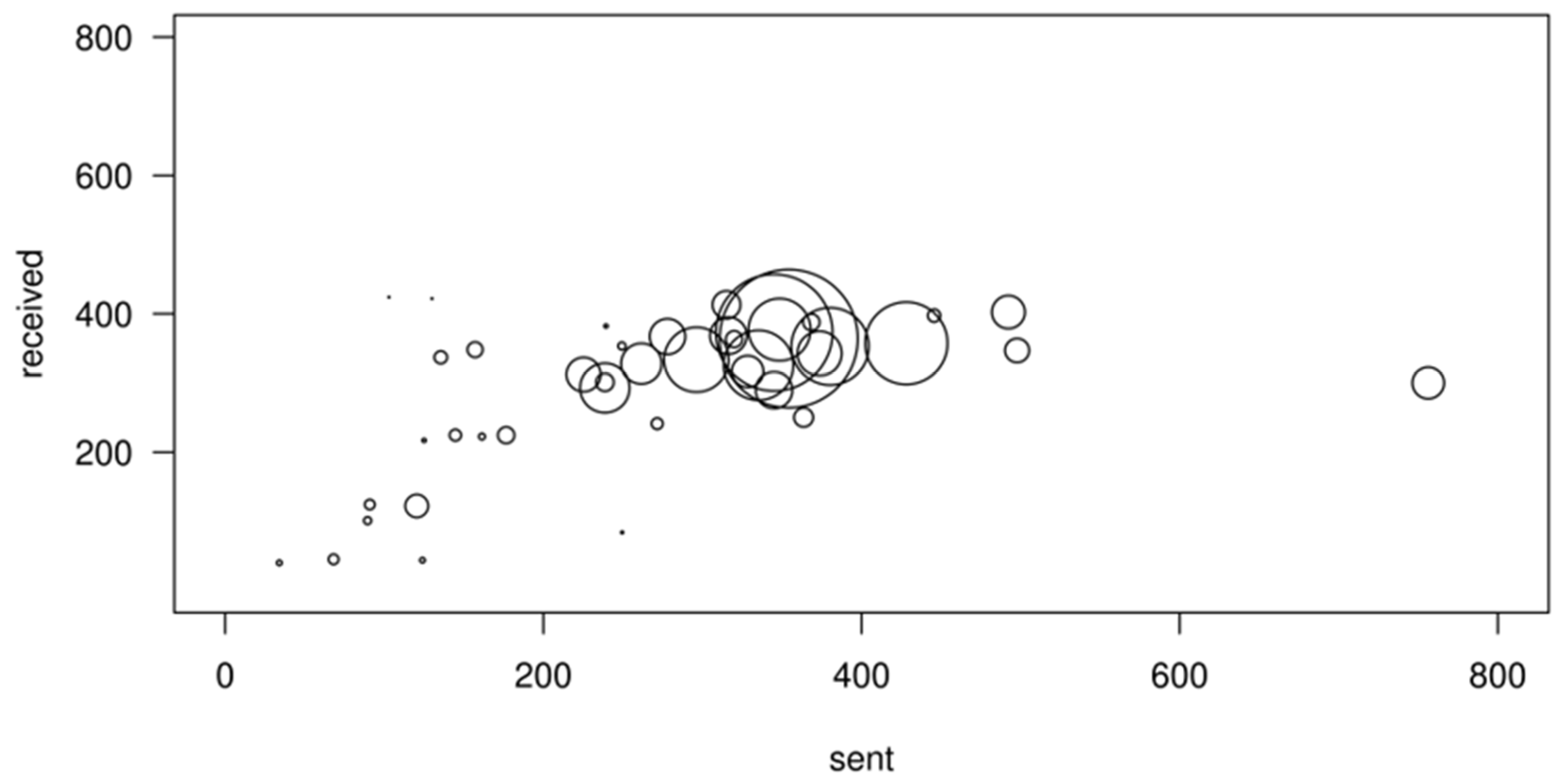
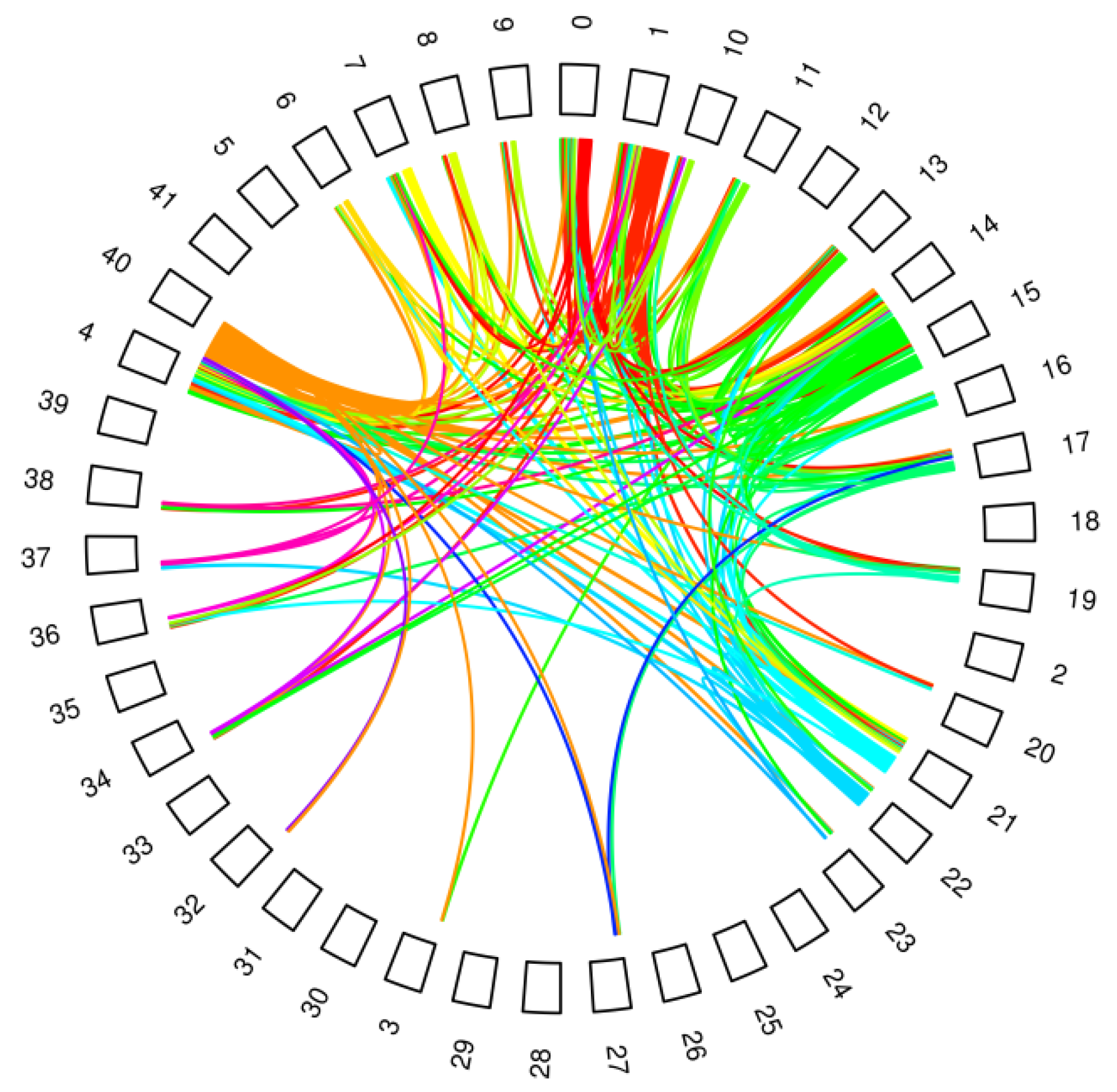
3. Email Network Data and Main Indicators
4. Graph Theory Indicators
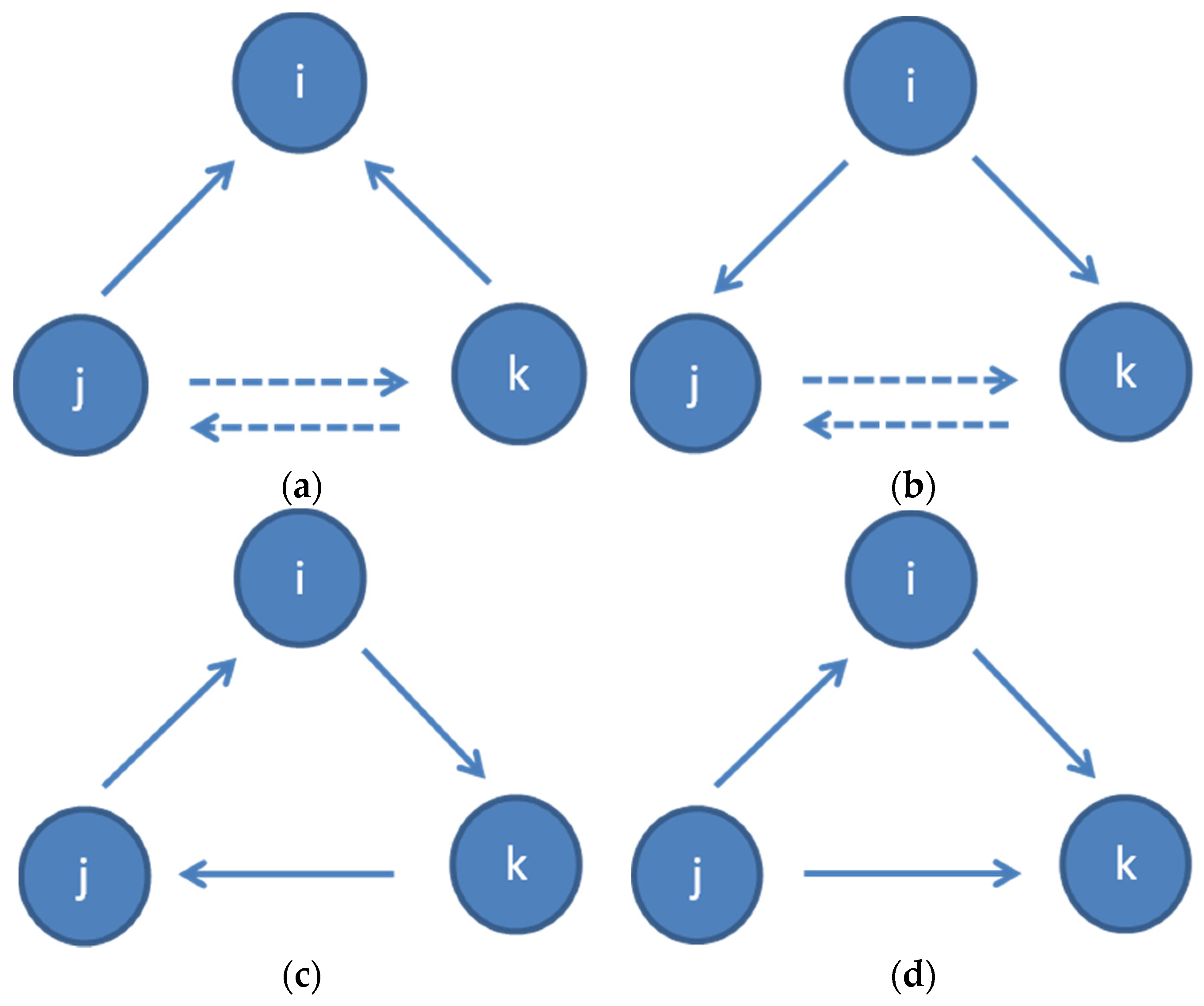
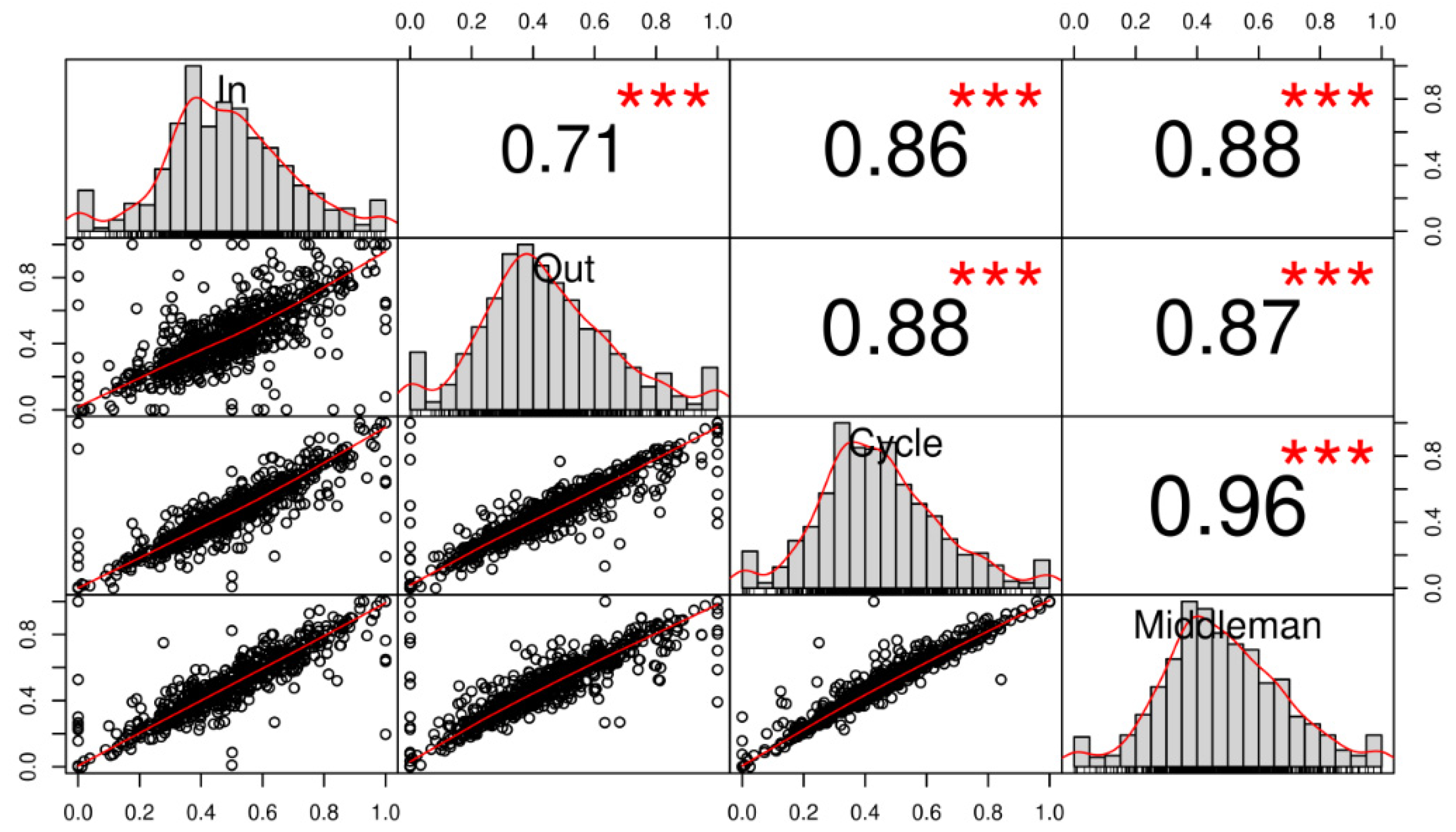
5. Extending Clustering Approach
- Cycle: a triangle where every arc has the same direction (j→i, i→k, k→ j or vice versa) (Figure 4c); and
- Middleman: a triangle where the two arcs of i have different directions and there is an arc between j and k (or vice versa), without forming a cycle. There are two arcs incoming to k or j (j→i, i→k, j→k or vice versa) (Figure 4d).
6. Symmetrical and A-Symmetrical Models
- Conventional model: independent variables include main statistics on individual email activity (number of emails sent and share of own replies within the threshold period) and standard symmetric centrality indicators;
- Clustering model: independent variables include main statistics on individual email activity and directed clustering indicators; and
- Extended Directional model: independent variables combine main statistics on individual email activity, directed centrality indicators, and directed clustering indicators.
6.1. Share of Outgoing Emails Responded Within 7 Days
6.2. Share of Outgoing Emails Responded Within 24 Hours
6.3. Validation of Methodology on Alternative Datasets
7. Conclusions
Funding
Conflicts of Interest
Appendix A. Results for Validation Networks

| Conventional | Clustering | Extended Directional | ||||
|---|---|---|---|---|---|---|
| Estimate | Pr(>|t|) | Estimate | Pr(>|t|) | Estimate | Pr(>|t|) | |
| Number of emails sent | −1.113 × 10⁻⁴ | 0.00601 ** | 1.403 × 10⁻⁴ | 0.000995 *** | −8.578 × 10⁻⁶ | 0.87386 |
| Share of own replies within period | 9.635 × 10⁻² | 0.04899 * | 9.553 × 10⁻¹ | <2 × 10⁻¹⁶ *** | 9.887 × 10⁻² | 0.04459 * |
| Closeness | 2.949 | <2 × 10⁻¹⁶ *** | ||||
| Closeness (in) | 4.887 × 10⁻² | 0.21796 | ||||
| Closeness (out) | −2.439 | 0.20323 | ||||
| “In” clustering coefficient | 1.245 × 10⁻¹ | 0.004622 ** | 4.887 × 10⁻² | 0.21796 | ||
| “Out” clustering coefficient | 4.702 × 10⁻³ | 0.878011 | −2.164 × 10⁻² | 0.43262 | ||
| “Middleman” clustering coefficient | −4.740 × 10⁻² | 0.272049 | −1.180 × 10⁻² | 0.76112 | ||
| Adjusted R-squared | 0.9823 | 0.9781 | 0.9823 | |||
| p-value | <2.2 × 10⁻¹⁶ | <2.2 × 10⁻¹⁶ | <2.2 × 10⁻¹⁶ | |||
| Conventional | Clustering | Extended Directional | ||||
|---|---|---|---|---|---|---|
| Estimate | Pr(>|t|) | Estimate | Pr(>|t|) | Estimate | Pr(>|t|) | |
| Number of emails sent | −9.079 × 10⁻⁵ | 0.085. | 2.369 × 10⁻⁴ | 0.000206 *** | 7.396 × 10⁻⁵ | 0.30228 |
| Share of own replies within period | 1.813 × 10⁻¹ | 3.69 × 10⁻¹⁰ *** | 9.111 × 10⁻¹ | <2 × 10⁻¹⁶ *** | 1.866 × 10⁻¹ | 1.04 × 10⁻¹⁰ *** |
| Closeness | 2.396 | <2 × 10⁻¹⁶ *** | ||||
| Closeness (in) | 8.495 | 0.00103 ** | ||||
| Closeness (out) | −6.139 | 0.01784 * | ||||
| “In” clustering coefficient | 1.529 × 10⁻¹ | 0.020532 * | 4.493 × 10⁻² | 0.40060 | ||
| “Out” clustering coefficient | −1.161 × 10⁻¹ | 0.011989 * | −9.589 × 10⁻² | 0.01030 * | ||
| “Middleman” clustering coefficient | 8.458 × 10⁻² | 0.192056 | 4.440 × 10⁻² | 0.39701 | ||
| Adjusted R-squared | 0.9607 | 0.9404 | 0.9611 | |||
| p-value | <2.2 × 10⁻¹⁶ | <2.2 × 10⁻¹⁶ | <2.2 × 10⁻¹⁶ | |||
| Conventional | Clustering | Extended Directional | ||||
|---|---|---|---|---|---|---|
| Estimate | Pr(>|t|) | Estimate | Pr(>|t|) | Estimate | Pr(>|t|) | |
| Number of emails sent | 2.161 × 10⁻⁵ | 0.462 | 1.245 × 10⁻⁴ | 6.72 × 10⁻⁵ *** | 1.413 × 10⁻⁵ | 0.742 |
| Share of own replies within period | 4.322 × 10⁻² | 4.481 × 10⁻² | 5.021 × 10⁻¹ | <2 × 10⁻¹⁶ *** | 3.915 × 10⁻² | 0.384 |
| Closeness | 1.482 | 1.201 × 10⁻¹ | ||||
| Closeness (in) | −1.107 × 101 | 0.881 | ||||
| Closeness (out) | 1.262 × 101 | 0.865 | ||||
| “In” clustering coefficient | 3.834 × 10⁻² | 0.521 | −1.115 × 10⁻¹ | 0.046 * | ||
| “Out” clustering coefficient | 1.761 × 10⁻¹ | 0.145 | 8.092 × 10⁻² | 0.461 | ||
| “Middleman” clustering coefficient | 7.172 × 10⁻² | 0.644 | 3.361 × 10⁻² | 0.739 | ||
| Adjusted R-squared | 0.6082 | 0.5239 | 0.6091 | |||
| p-value | <2.2 × 10⁻¹⁶ | <2.2 × 10⁻¹⁶ | <2.2 × 10⁻¹⁶ | |||
| Conventional | Clustering | Extended Directional | ||||
|---|---|---|---|---|---|---|
| Estimate | Pr(>|t|) | Estimate | Pr(>|t|) | Estimate | Pr(>|t|) | |
| Number of emails sent | 1.154 × 10⁻⁵ | 8.94 × 10⁻⁶ *** | 1.208 × 10⁻⁵ | 1.69 × 10⁻⁶ *** | 3.523 × 10⁻⁶ | 0.35463 |
| Share of own replies within period | 6.126 × 10⁻¹ | <2 × 10⁻¹⁶ *** | 6.149 × 10⁻¹ | <2 × 10⁻¹⁶ *** | 6.110 × 10⁻¹ | <2 × 10⁻¹⁶ *** |
| Closeness | 3.245 × 10⁻³ | 0.492 | ||||
| Closeness (in) | −1.847 × 101 | 0.00524 ** | ||||
| Closeness (out) | 1.847 × 101 | 0.00522 ** | ||||
| “In” clustering coefficient | −2.139 × 10⁻⁴ | 0.964 | −3.092 × 10⁻³ | 0.53343 | ||
| “Out” clustering coefficient | 1.449 × 10⁻³ | 0.883 | 1.779 × 10⁻³ | 0.85563 | ||
| “Middleman” clustering coefficient | −1.584 × 10⁻³ | 0.860 | −2.073 × 10⁻³ | 0.81785 | ||
| Adjusted R-squared | 0.6791 | 0.678 | 0.6814 | |||
| p-value | <2.2 × 10⁻¹⁶ | <2.2 × 10⁻¹⁶ | <2.2 × 10⁻¹⁶ | |||
References
- Zhong, S.; Geng, Y.; Liu, W.; Gao, C.; Chen, W. A bibliometric review on natural resource accounting during 1995–2014. J. Clean. Prod. 2016, 139, 122–132. [Google Scholar] [CrossRef]
- Christodoulou, A.; Christidis, P. Measuring cross-border road accessibility in the European Union. Sustainability 2019, 11, 4000. [Google Scholar] [CrossRef] [Green Version]
- Kim, J.; Hastak, M. Social network analysis: Characteristics of online social networks after a disaster. Int. J. Inf. Manag. 2018, 38, 86–96. [Google Scholar] [CrossRef]
- De Mesa, E.G.; Hidalgo, I.; Christidis, P.; Ciscar, J.C.; Vegas, E.; Ibarreta, D. Modeling the impact of genetic screening technologies on healthcare: Theoretical model for asthma in children. Mol. Diagn. Ther. 2007, 11, 313–323. [Google Scholar] [CrossRef] [PubMed]
- Christidis, P. Four shades of Open Skies: European Union and four main external partners. J. Transp. Geogr. 2016, 50, 105–114. [Google Scholar] [CrossRef]
- Pan, Y.; Tan, W.; Chen, Y. The analysis of key nodes in complex social networks, Lecture Notes in Computer Science (including subseries Lecture Notes in Artificial Intelligence and Lecture Notes in Bioinformatics). LNCS 2017, 10603, 829–836. [Google Scholar]
- Christidis, P.; Losada, A.G. Email based institutional network analysis: Applications and risks. Soc. Sci. 2019, 8, 306. [Google Scholar] [CrossRef] [Green Version]
- Lazer, D.; Pentland, A.; Adamic, L.; Aral, S.; Barabasi, A.L.; Brewer, D.; Christakis, N.; Contractor, N.; Fowler, J.; Myron, G.; et al. Social science: Computational social science. Science 2009, 323, 721–723. [Google Scholar] [CrossRef] [Green Version]
- Benson, A.R.; Gleich, D.F.; Leskovec, J. Higher-order organization of complex networks. Science 2016, 353, 163–166. [Google Scholar] [CrossRef] [Green Version]
- Clemente, G.P.; Grassi, R. Directed clustering in weighted networks: A new perspective. Chaos Solitons Fractals 2018, 107, 26–38. [Google Scholar] [CrossRef] [Green Version]
- Clemente, G.P.; Grassi, R. Directed Weighted Clustering Coefficient (Package ‘DirectedClustering’). 2018. Available online: https://cran.r-project.org/web/packages/DirectedClustering/DirectedClustering.pdf (accessed on 31 March 2020).
- Adamic, L.A.; Adar, E. Friends and neighbors on the web. Soc. Netw. 2001, 25, 211–230. [Google Scholar] [CrossRef] [Green Version]
- Barrat, A.; Barthelemy, M.; Pastor-Satorras, R.; Vespignani, A. The architecture of complex weighted networks. Proc. Natl. Acad. Sci. USA 2004, 101, 3747. [Google Scholar] [CrossRef] [PubMed] [Green Version]
- Watts, D.; Strogatz, S. Collective dynamics of ‘small-world’ networks. Nature 1998, 393, 440–442. [Google Scholar] [CrossRef] [PubMed]
- Fagiolo, G. Clustering in complex directed networks. Phys. Rev. E 2007, 76, 026107. [Google Scholar] [CrossRef] [PubMed] [Green Version]
- Fagiolo, G.; Reyes, J.; Schiavo, S. World-trade web: Topological properties, dynamics, and evolution, Physical Review E—Statistical. Phys. Rev. E Stat. Nonlin. Soft Matter Phys. 2008, 79, 036115. [Google Scholar]
- Traud, A.L.; Mucha, P.J.; Porter, M.A. Social structure of Facebook networks. Phys. A 2012, 391, 4165–4180. [Google Scholar] [CrossRef] [Green Version]
- Chen, D.B.; Gao, H.; Lü, L.; Zhou, T. Identifying influential nodes in large-scale directed networks: The role of clustering. PLoS ONE 2013, 8, 0077455. [Google Scholar] [CrossRef] [Green Version]
- Myers, S.A.; Sharma, A.; Gupta, P.; Lin, J. Information network or social network? The structure of the twitter follow graph, WWW 2014 Companion. In Proceedings of the 23rd International Conference on World Wide Web, Seoul, Korea, 7–11 April 2014; pp. 493–498. [Google Scholar]
- Hangal, S.; MacLean, D.; Lam, M.; Heer, J. All Friends are Not Equal: Using Weights in Social Graphs to Improve Search. In Proceedings of the Fourth ACM Workshop on Social Network Mining and Analysis Held in Conjunction with ACM SIGKDD International Conference on Knowledge Discovery and Data Mining (KDD), Washington, DC, USA, 24–28 July 2010. [Google Scholar]
- Portela, J.; Villalba, L.J.G.; Silva Trujillo, A.G.; Sandoval Orozco, A.L.; Kim, T.-H. Estimation of anonymous email network characteristics through statistical disclosure attacks. Sensors 2016, 16, 1832. [Google Scholar] [CrossRef]
- Chen, Q.; Su, H.; Liu, J.; Yan, B.; Zheng, H.; Zhao, H. In Pursuit of social capital: Upgrading social circle through edge rewiring. Web Big Data 2019. [Google Scholar] [CrossRef]
- Tang, J.; Lou, T.; Kleinberg, J. Inferring social ties across heterogenous networks. In Proceedings of the Fifth ACM International Conference on Web Search and Data Mining, ACM, Washington, DC, USA, 8–12 February 2012; pp. 743–752. [Google Scholar]
- Chen, R. Living a private life in public social networks: An exploration of member self-disclosure. Decis. Support Syst. 2013, 55, 661–668. [Google Scholar] [CrossRef]
- Saqr, M.; Fors, U.; Nouri, J. Using social network analysis to understand online problem-based learning and predict performance. PLoS ONE 2018, 13, e0203590. [Google Scholar] [CrossRef] [PubMed] [Green Version]
- Yin, H.; Benson, A.R.; Leskovec, J.; Gleich, D.F. Local Higher-order Graph Clustering. In Proceedings of the 23rd ACM SIGKDD International Conference on Knowledge Discovery and Data Mining, New York, NY, USA, 13–17 August 2017. [Google Scholar]
- Leskovec, J.; Kleinberg, J.; Faloutsos, C. Graph Evolution: Densification and Shrinking Diameters. Acm Tkdd 2007, 1, 2-es. [Google Scholar] [CrossRef]
- Freeman, L.C. Centrality in networks: I. Conceptual clarification. Soc. Netw. 1979, 1, 215–239. [Google Scholar] [CrossRef] [Green Version]
- Marsden, P. Measures of Network Centrality. In International Encyclopedia of the Social & Behavioral Sciences, 2nd ed.; Elsevier: Amsterdam, The Netherlands, 2015; pp. 532–539. [Google Scholar]
- Bavelas, A. Communication patterns in task-oriented groups. J. Acoust. Soc. Am. 1950, 22, 725–730. [Google Scholar] [CrossRef]
- Marchiori, M.; Latora, V. Harmony in the small-world. Phys. A 2000, 285, 539–546. [Google Scholar] [CrossRef] [Green Version]
- Csardi, G.; Nepusz, T. The igraph software package for complex network research. Int. J. Complex Syst. 2006, 1695, 1–9. [Google Scholar]
- Opsahl, T.; Panzarasa, P. Clustering in Weighted Networks. Soc. Netw. 2009, 31, 155–163. [Google Scholar] [CrossRef]
- Shinkuma, R.; Sugimoto, Y.; Inagaki, Y. Weighted network graph for interpersonal communication with temporal regularity. Soft Comput. 2019, 23, 3037–3051. [Google Scholar] [CrossRef] [Green Version]
- Panzarasa, P.; Opsahl, T.; Carley, K. Patterns and dynamics of users’ behavior and interaction: Network analysis of an online community. J. Am. Soc. Inf. Sci. Technol. 2009, 60, 911–932. [Google Scholar] [CrossRef]
- Klimmt, B.; Yang, Y. Introducing the Enron Corpus, CEAS Conference. 2004. Available online: http://ceas.cc/2004/168.pdf (accessed on 31 March 2020).


| Authors | Network | Indicators | Directed | Weights |
|---|---|---|---|---|
| Adamic and Adar (2001) [12] | Web page network | Structural | Yes | Structural (number of links) |
| Watts and Strogatz (1998) [14] | Biological network; Collaboration network | Clustering | No | No |
| Barrat et al. (2004) [13] | Aviation network | Structural; Activity | yes | Activity (available seats per year) |
| Fagiolo (2007) [15] | International trade network | Clustering | Yes | Clustering (unweighted local coefficients) |
| Fagiolo et al. (2008) [16] | International trade network | Structural; Activity; Clustering | Yes | Clustering (weighted local coefficients) |
| Hangal et al. (2010) | Bibliography network; Twitter retweet network | Structural; Activity | Yes | Activity (directed influence between nodes) |
| Traud et al. (2012) [17] | Facebook contacts network | Structural; Clustering | No | No |
| Chen et al. (2013) [18] | Online community network; collaboration network | Clustering | Yes | Clustering (in- and out-degree) |
| Myers et al. (2014) [19] | Twitter follow graph | Structural; Clustering | Yes | No |
| Clemente and Grassi (2018) [11] | Theoretical graphs | Clustering | Yes | Clustering (weighted local coefficients) |
| Portela et al. (2016) [21] | email network | Structural; Clustering | Yes | No |
| Chen et al. (2019) [22] | email network | Structural | Yes | No |
| This work | email network | Structural; Activity; Clustering | Yes | Clustering (weighted local coefficients, based on References [21,22]) |
| Indicator | Median | Mean | Minimum | Maximum | Standard Deviation | Skewness |
|---|---|---|---|---|---|---|
| Number of sent emails | 77 | 330.7 | 0 | 9782 | 740.4 | 5.43 |
| Number of received emails | 130 | 330.7 | 0 | 4710 | 483.9 | 2.88 |
| Ratio of number of sent to number of received emails | 0.767 | 1.553 | 0.002 | 303.6 | 11.43 | 25.11 |
| Indicator | Median | Mean | Minimum | Maximum | Standard Deviation | Skewness |
|---|---|---|---|---|---|---|
| Number of sent emails per person | 378.75 | 370.67 | 43.33 | 970.47 | 197.69 | 0.85 |
| Number of received emails per person | 423 | 392.63 | 52.67 | 640 | 146.89 | −0.61 |
| Ratio of number of sent to number of received emails | 0.90 | 1.02 | 0.24 | 2.88 | 0.552 | 1.8 |
| Median | Mean | Minimum | Maximum | Standard Deviation | Skewness | |
|---|---|---|---|---|---|---|
| Degree centrality | 0.0478 | 0.0657 | 0.0020 | 0.5483 | 0.0623 | 2.34 |
| Degree centrality (in) | 0.0244 | 0.0322 | 0.0010 | 0.2116 | 0.0287 | 1.98 |
| Degree centrality (out) | 0.0234 | 0.0336 | 0.0010 | 0.3367 | 0.0349 | 2.72 |
| Closeness centrality | 0.3759 | 0.3787 | 0.3699 | 0.4692 | 0.0091 | 3.18 |
| Closeness centrality (in) | 0.3752 | 0.3779 | 0.3699 | 0.4692 | 0.0073 | 2.19 |
| Closeness centrality (out) | 0.3755 | 0.3775 | 0.3699 | 0.4265 | 0.0091 | 3.30 |
| Betweenness centrality | 958 | 2453.9 | 0 | 42,250 | 4449.6 | 4.40 |
| Betweenness centrality (directional) | 956 | 2446.6 | 0 | 42,225 | 4437.5 | 4.41 |
| Clustering Coefficient | Median | Mean | Minimum | Maximum | Standard Deviation | Skewness |
|---|---|---|---|---|---|---|
| In | 0.4738 | 0.4828 | 0 | 1 | 0.2026 | 0.1466 |
| Out | 0.4167 | 0.4413 | 0 | 1 | 0.2141 | 0.4148 |
| Middleman | 0.4689 | 0.4845 | 0 | 1 | 0.1988 | 0.2346 |
| Cycle | 0.4282 | 0.4444 | 0 | 1 | 0.1963 | 0.4019 |
| n | k | From | To | Timestamp | ||
|---|---|---|---|---|---|---|
| 1 | 1 | i | j | t1 | t2–t1 | |
| 2 | j | i | t2 | |||
| 3 | 2 | i | j | t3 | t3–t2 | |
| 4 | 3 | i | j | t4 | t5–t4 | |
| 5 | j | i | t5 | |||
| 6 | 4 | i | j | t6 | t6–t5 |
| Conventional | Clustering | Extended Directional | ||||
|---|---|---|---|---|---|---|
| Estimate | Pr(>|t|) | Estimate | Pr(>|t|) | Estimate | Pr(>|t|) | |
| Number of emails sent | 1.294 × 10⁻⁴ | <2 × 10⁻¹⁶ *** | 1.396 × 10⁻⁴ | <2 × 10⁻¹⁶ *** | 1.069 × 10⁻¹⁶ | <2 × 10⁻¹⁶ *** |
| Share of own replies within period | 4.174 × 10⁻¹ | <2 × 10⁻¹⁶ *** | 5.713 × 10⁻¹ | <2 × 10⁻¹⁶ *** | 4.676 × 10⁻¹ | <2 × 10⁻¹⁶ *** |
| Closeness | 4.201 × 10⁻¹ | 3.51 × 10⁻¹⁶ ****** | ||||
| Closeness (in) | −1.223 × 101 | 6.44 × 10⁻¹⁰ *** | ||||
| Closeness (out) | 1.259 × 101 | 1.51 × 10⁻¹⁰ *** | ||||
| “In” clustering coefficient | 3.953 × 10⁻¹ | 1.55 × 10⁻⁷ *** | 2.757 × 10⁻¹ | 0.000130 *** | ||
| “Out” clustering coefficient | 2.208 × 10⁻¹ | 0.00121 ** | 2.519 × 10⁻¹ | 0.000102 *** | ||
| “Middleman” clustering coefficient | −4.599 × 10⁻¹ | 2.14 × 10⁻⁵ *** | −5.004 × 10⁻¹ | 1.43 × 10⁻⁶ *** | ||
| Adjusted R-squared | 0.8468 | 0.8428 | 0.8596 | |||
| p-value | <2.2 × 10⁻¹⁶ | <2.2 × 10⁻¹⁶ | <2.2 × 10⁻¹⁶ | |||
| Conventional | Clustering | Extended Directional | ||||
|---|---|---|---|---|---|---|
| Estimate | Pr(>|t|) | Estimate | Pr(>|t|) | Estimate | Pr(>|t|) | |
| Number of emails sent | 9.420 × 10⁻⁵ | <2 × 10⁻¹⁶ *** | 1.065 × 10⁻⁴ | <2 × 10⁻¹⁶ *** | 7.913 × 10⁻⁵ | <2 × 10⁻¹⁶ *** |
| Share of own replies within period | 3.163 × 10⁻¹ | <2 × 10⁻¹⁶ *** | 4.499 × 10⁻¹ | <2 × 10⁻¹⁶ *** | 3.492 × 10⁻¹ | <2 × 10⁻¹⁶ *** |
| Closeness | 3.001 × 10⁻¹ | <2 × 10⁻¹⁶ *** | ||||
| Closeness (in) | −7.363 | 3.01 × 10⁻⁶ *** | ||||
| Closeness (out) | 7.687 | 9.58 × 10⁻⁷ *** | ||||
| “In” clustering coefficient | 2.782 × 10⁻¹ | 3.94 × 10⁻⁶ *** | 1.769 × 10⁻¹ | 0.002354 ** | ||
| “Out” clustering coefficient | 1.598 × 10⁻¹ | 0.003591 ** | 1.726 × 10⁻¹ | 0.000991 *** | ||
| “Middleman” clustering coefficient | −3.137 × 10⁻¹ | 0.000312 *** | −3.662 × 10⁻¹ | 1.28 × 10⁻⁵ *** | ||
| Adjusted R-squared | 0.7675 | 0.7571 | 0.7806 | |||
| p-value | <2.2 × 10⁻¹⁶ | <2.2 × 10⁻¹⁶ | <2.2 × 10⁻¹⁶ | |||
| Conventional | Clustering | Extended Directional | ||||
|---|---|---|---|---|---|---|
| 7 D | 1 D | 7 D | 1 D | 7 D | 1 D | |
| email-Eu-core-temporal | 0.8468 | 0.7675 | 0.8428 | 0.7571 | 0.8596 | 0.7806 |
| CollegeMsg | 0.9823 | 0.9607 | 0.9781 | 0.9404 | 0.9823 | 0.9611 |
| Enron | 0.6082 | 0.6791 | 0.5239 | 0.678 | 0.6091 | 0.6818 |
| Email-Eu-Core-Temporal | CollegeMsg | Enron | ||||
|---|---|---|---|---|---|---|
| 7 D | 1 D | 7 D | 1 D | 7 D | 1 D | |
| Number of emails sent | + * | + * | - | + | + | + |
| Share of own replies within period | + * | + * | + * | + * | + | + * |
| Closeness (in) | - * | - * | + | + * | - | - * |
| Closeness (out) | + * | + * | - | - * | + | + * |
| “In” clustering | + * | + * | + | + | - | - |
| “Out” clustering | + * | + * | - | - * | + | + |
| “Middleman” clustering | - * | - * | - | + | + | - |
© 2020 by the author. Licensee MDPI, Basel, Switzerland. This article is an open access article distributed under the terms and conditions of the Creative Commons Attribution (CC BY) license (http://creativecommons.org/licenses/by/4.0/).
Share and Cite
Christidis, P. Intensity of Bilateral Contacts in Social Network Analysis. Information 2020, 11, 189. https://doi.org/10.3390/info11040189
Christidis P. Intensity of Bilateral Contacts in Social Network Analysis. Information. 2020; 11(4):189. https://doi.org/10.3390/info11040189
Chicago/Turabian StyleChristidis, Panayotis. 2020. "Intensity of Bilateral Contacts in Social Network Analysis" Information 11, no. 4: 189. https://doi.org/10.3390/info11040189
APA StyleChristidis, P. (2020). Intensity of Bilateral Contacts in Social Network Analysis. Information, 11(4), 189. https://doi.org/10.3390/info11040189