Mean Received Resources Meet Machine Learning Algorithms to Improve Link Prediction Methods

Abstract

The analysis of social networks has attracted a lot of attention during the last two decades. These networks are dynamic: new links appear and disappear. Link prediction is the problem of inferring links that will appear in the future from the actual state of the network. We use information from nodes and edges and calculate the similarity between users. The more users are similar, the higher the probability of their connection in the future will be. The similarity metrics play an important role in the link prediction field. Due to their simplicity and flexibility, many authors have proposed several metrics such as Jaccard, AA, and Katz and evaluated them using the area under the curve (AUC). In this paper, we propose a new parameterized method to enhance the AUC value of the link prediction metrics by combining them with the mean received resources (MRRs). Experiments show that the proposed method improves the performance of the state-of-the-art metrics. Moreover, we used machine learning algorithms to classify links and confirm the efficiency of the proposed combination.

1. Introduction

Many real-world complex systems are represented by graphs, where nodes are entities such as universities, people or even proteins and edges represents the relations between the nodes. The most central property of these networks is their evolution, where edges are added and deleted over time. Link prediction (LP) is one of the most important tasks in social network analysis. It has many applications in various areas: spam E-mail [1]; disease prediction [2]; system recommendations [3]; and viral marketing [4]. The authors in [5] used a network-based technique to assess multimorbidity data and build algorithms for forecasting which diseases a patient is likely to develop in their research. A temporal bipartite network is used to describe multimorbidity data, with nodes representing patients and diseases, and a link between these nodes indicating that the patient has been diagnosed with the condition. The link prediction problem is defined as: let G(V,E) be an undirected graph, V is the set of nodes that refer to users of a social network (SN), E is the set of links or edges that represent relations between nodes. Given a snapshot of links at time t, could we infer the links that will be established at time $t+\Delta t$?

To solve this issue, authors have proposed various approaches. The authors in [6] have compared several similarity measures using AUC, and their results show that the Adamic Adar metric (AA) [7] performs best in four of the five datasets followed by Jaccard [8]; the difference between those two metrics is that (AA) [7] assumes that the rare common neighbors are heavily weighted; however, Jaccard [8] measures the probability that two nodes have a common neighbor. The authors in [9] have an proposed adaptive degree penalization metric (ADP). They proposed a generalized formula for the existing degree penalization local link prediction method in order to provide the degree penalization level. Then, the penalization parameter for a network is predicted using logistic regression. In [10,11], we proposed a similarity metric based on the path depth from a source node to a destination node and their degrees. In addition, we found a strong correlation between the clustering coefficient and area under the curve. Machine learning algorithms were used to solve the link prediction problem where the enhancement was by $40\%$ in the power grid dataset.

In [12], the authors solved the link prediction problem as a binary classification task, where they set the precision as an objective function, and then transform the link prediction problem into an optimization problem where the authors defined a feature set for each edge. This set contains state-of-the-art metrics, the used class label was $+1$ for existing links and $-1$ for non-existing links. In [13], the authors collected four different data, namely: node feature subset, topology features subset, social features subset (following or followed) and collaborative filtering for the voting feature subset, then they trained SVM, naive Bayes, random forest and logistic regression classifiers. In [14], the authors used the importance of neighborhood knowledge in link prediction that has been proven. As a result, they suggest extracting structural information from input samples using a neighborhood neural encoder.

In [15], the authors proposed a combination of the preferential attachment metric (PA) and (AA) to solve the link prediction problem using weights for each used metric and then obtained good accuracy for the GitHub dataset: $S_{comb}(x,y)=0.7*s_{PA}(x,y)+0.3*s_{AA}(x,y)$. The same idea was applied in [16] where the authors proposed common neighbor and centrality-based parameterized algorithm (CCPA): $S_{xy}=\alpha \times (\Gamma \left(x\right)\cap \Gamma \left(y\right))+(1-\alpha )\times \frac{N}{d_{xy}}$, $\alpha$ is a parameter between $[0;1]$. It is used to control the weight of common neighbors and centrality, $\Gamma \left(x\right)$ represents the neighbors of node x, the fraction $\frac{N}{d_{xy}}$ represents the closeness centrality between the nodes x and y, where N is the number of nodes in the network, and $d_{xy}$ is the shortest path between x and y.

As shown previously, recent decades have witnessed a tremendous growth in the amount of research seeking to provide precise predictions of links. Researchers have only focused on proposing new metrics and compared their results using area under the curve (AUC) against the state-of-the-art metrics. However, there is still a need for a unique method that enables the users of state-of-the-art metrics to improve their results in terms of accuracy. This paper proposes a solution to a link prediction (LP) problem based on the combination of state-of-the-art metrics and mean received resources (MRRs). This method is parameterized to grant full control to the user/system to give the importance to the link prediction metric or the MRRs. The main goal is to improve the area under the curve (AUC) of the state-of-the-art measures and any other local metric that could or will be proposed. We proved that the proposed combination has a meaningful effect on the results. Then, we used machine learning algorithms to classify the links. The results show the superiority of machine learning models whenever we add our proposed metric as an additional feature. Furthermore, we found that the decision tree performs best using the proposed metric.

To summarize, the principal contributions of this paper are:

• We proposed a new parameterized link prediction metric that grants the user or system the full control of metric. Note that the proposed metric enhances the performance of the state-of-the-art metrics;
• We compared the performance of the proposed metric against the state-of-the-art metrics using the AUC;
• We studied the impact of using the parameter on each enhanced version of link prediction;
• We studied the correlation between the parameter and the network features;
• We used machine learning algorithms to confirm the efficiency of the proposed method.

This paper is organized as follows: in Section 2, we describe the state-of-the-art metrics and introduce the proposed metric. Section 3 presents the evaluation metric AUC and the datasets used to compare the proposed metric with the state-of-the-art metrics. In Section 4, we report the results. In Section 5, we used machine learning algorithms to classify the links. We conclude our paper in Section 6.

2. Methods

In this section, we introduce the state-of-the-art metrics, particularly the local metrics, their merits and drawbacks. Then, we present the proposed metric which is based on the mean received resources and a local similarity metric.

2.1. Related Works

According to [17], the authors classified the link prediction approaches into three major categories. In the first approach, link prediction is solved using the dimensionality reduction, the second approach relies on probabilistic and maximum likelihood models (note that we cannot use the first and second category of approaches for large-scale networks because of their high computational cost), the last approach uses similarity-based methods, which is divided into three sub-categories, namely: global metrics, quasi-local metrics and local similarity metrics. The most used metrics are local metrics because of their reasonable computational coast and the high AUC results they provide; some of these metrics are designed for a specific domain (such as cosine similarity, which is used in information retrieval and text mining [18]).

In this work, we only focused on local metrics, also known as neighborhood-based metrics (see Table 1). Through this paper, we use $e_{x,y}$ to refer to the link between nodes x and y, $\Gamma \left(x\right)$ is the set of neighbors of x. $|\Gamma (x\left)\right|$ is the degree of node x (how many neighbors the node x has). ShortestPaths(x,y) is the set of all shortest paths between x and y.

Table 1. Neighborhood-based similarity metrics.

Metric Name	Equation
Preferential attachment (PA) [19]	$$PA(x,y)=|\Gamma (x\left)\right|·|\Gamma (y\left)\right|$$ (1)
Common neighbor (CN) [20]	$$CN(x,y)=|\Gamma (x)\cap \Gamma (y\left)\right|$$ (2)
Hub promoted (HP) [21]	$$HP(x,y)=\frac{|\Gamma (x)\cap \Gamma (y\left)\right|}{min\left\{\right|\Gamma \left(x\right)|,|\Gamma \left(y\right)\left|\right\}}$$ (3)
Hub depressed (HD) [21]	$$HD(x,y)=\frac{|\Gamma (x)\cap \Gamma (y\left)\right|}{max\left\{\right|\Gamma \left(x\right)|,|\Gamma \left(y\right)\left|\right\}}$$ (4)
Jaccard coefficient (JA) [8]	$$JA(x,y)=\frac{|\Gamma (x)\cap \Gamma (y\left)\right|}{|\Gamma (x)\cup \Gamma (y\left)\right|}$$ (5)
Leicht–Holme–Nerman (LHN) [22]	$$LHN(x,y)=\frac{|\Gamma (x)\cap \Gamma (y\left)\right|}{|\Gamma (x\left)\right|·|\Gamma (y\left)\right|}$$ (6)
Parameter dependent (PD) [23]	$$PD(x,y)=\frac{\Gamma \left(x\right)\cap \Gamma \left(y\right)}{{(\Gamma \left(x\right)·\Gamma \left(y\right))}^{\delta }}$$ (7)
Adamic/Adar (AA) [7]	$$AA(x,y)=\sum _{z\in |\Gamma (x)\cap \Gamma (y\left)\right|}\frac{1}{log|\Gamma (z\left)\right|}$$ (8)
Salton [24]	$$Salton(x,y)=\frac{|\Gamma (x)\cap \Gamma (y\left)\right|}{\sqrt{|\Gamma (x\left)\right|·|\Gamma (y\left)\right|}}$$ (9)
Sorensen [25]	$$Sorensen(x,y)=\frac{2·|\Gamma (x)\cap \Gamma (y\left)\right|}{|\Gamma (x\left)\right|+|\Gamma (y\left)\right|}$$ (10)
Resource allocation (RA) [26]	$$RA(x,y)=\sum _{z\in \Gamma \left(x\right)\cap \Gamma \left(y\right)}\frac{1}{|\Gamma (z\left)\right|}$$ (11)

The neighborhood-based metrics presented in Table 1 rely on simple assumptions; for instance, the authors in [20] assumed that the more two nodes have common friends, the higher the probability is that they will be connected in the future. The authors in [19] assumed that the more both nodes have friends, the higher the probability that they will be connected. This assumption follows the principle “The rich get richer” from the field of economics. In conclusion, we can notice that each author has a different point of view with respect to this problem, but the end point is to provide a metric that performs well in term of AUC. The motivation of this work was to propose a new approach that enables researchers to power up the AUC of the metrics. We propose a parameterized expression based on the mean received resources MRR and a local metric. Note that we can apply the proposed enhancement to all the existing local metrics by adjusting the combination parameter for any type of dataset.

2.2. The Proposed Metric

Let G (V, E) be a simple graph (no loop or multiple edges are allowed). Motivated by the RA [26] index, where the authors used the flow of resources transferred from a source node to a destination node through common neighbors; considering two non-connected nodes A and B, the node A can transfer some resources (we assume that A has only one resource to share) to target node B, that the common neighbors play the role of transmitters, the node A distributes the resource to all their neighbors, and every neighbor will do the same until the resource reaches the node B. We extended this metric to a global scale and considered the mean received resources from the source node through the shortest paths. Because neighborhood-based metrics could not capture global relations, we used MRR as the second criterion to enhance the precision of the link prediction metrics previously introduced in Table 1. We define the mean received resources as

$$MR{R}_{A,B}=\frac{1}{|Shortest\_Paths(A,B\left)\right|}\times \sum _{path\in Shortest\_Paths(A,B)}\left(\prod _{node\in path}\frac{1}{|\Gamma (node\left)\right|}\right)$$

(12)

The following example describes one limitation of the neighbor-based metrics (such as resource allocation) and shows the advantages of the mean received approach. Let G (V, E) be a graph, x and y are two unconnected nodes. On the first hand, if $|\Gamma (x)\cap \Gamma (y\left)\right|=0$, then the resource allocation cannot capture the interaction between nodes x and y. On the other hand, the MRR will capture the interactions between x and y using the shortest paths. We clarify the problem with a simple graph of six nodes as shown in Figure 1. If we use the RA measure or any other neighbor-based metric presented in the previous section, then $s_{X,Y}=0$ (see Figure 1). However, the use of the mean received resources provides the capture of the interactions between the two nodes. There are three shortest paths between the two nodes $(x,y)$:

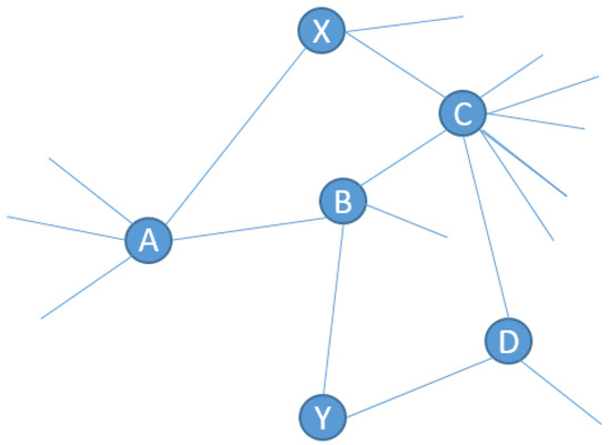
Figure 1. A simple undirected graph.

• The path through the nodes A and B:  $s_1=\frac{1}{\left|X\right|}\times \frac{1}{\left|A\right|}\times \frac{1}{\left|B\right|}\times \frac{1}{\left|Y\right|}=\frac{1}{3}\times \frac{1}{5}\times \frac{1}{4}\times \frac{1}{2}$
• The path through the nodes C and B:  $s_2=\frac{1}{\left|X\right|}\times \frac{1}{\left|C\right|}\times \frac{1}{\left|B\right|}\times \frac{1}{\left|Y\right|}=\frac{1}{3}\times \frac{1}{8}\times \frac{1}{4}\times \frac{1}{2}$
• The path through the nodes C and D:  $s_3=\frac{1}{\left|X\right|}\times \frac{1}{\left|C\right|}\times \frac{1}{\left|D\right|}\times \frac{1}{\left|Y\right|}=\frac{1}{3}\times \frac{1}{8}\times \frac{1}{3}\times \frac{1}{2}$

$MR{R}_{x,y}=\frac{1}{3}\times (s_1+s_2+s_3)$.

Each similarity measure captures different information data. The combination of these information data allows us to group them into a single equation and optimize the classification task. We power up each local measure (LM) presented in the previous subsection by combining them with Equation (12) using the weighted sum model (weighted combination [27]). We define the weighted combination as

$$PS{I}_{x,y}=\alpha \times sigmoid\left(LM(x,y)\right)+(1-\alpha )\times sigmoid\left(MRR(x,y)\right)$$

(13)

where $\alpha$ is a combination parameter, $\alpha \in [0;1]$. This parameter controls the contribution of each part of the equation; for some datasets, the MRR gives good results, but for others, the LM leads to higher prediction efficiency. Therefore, we used $\alpha$ to adjust the amount of contribution of each part. The MRR gives values in the range of $[0;1]$, however, other metrics such as CN provide values which are superior to 1. Therefore, we should normalize the local metric and MRR. To this end, we used the sigmoid function [28].

3. Evaluation

In this section, we introduce the methodology and the evaluation metric commonly used in the field. We define the datasets used to compare our metric against state-of-the-art metrics. We also describe the characteristics of each network.

3.1. Methodology

Each dataset is separated into two graphs: training $G_T$ and probe $G_P$, which are distinct and non-overlapping. The training graph $G_T$ is created by sampling the original graph G at random. $G_P$ is formed by the remaining edges that are not included in $G_T$. Similarly, the set of edges in $G_T$ refers to $E_T$, whereas those in $G_P$ are referred to as $E_P$, i.e., $E=E_T+E_P$. It is essential to mention that $E_T$ and $E_P$ are mutually exclusive. However, the nodes in $G_T$ and $G_P$ may overlap. For our experiments, $E_T$ represents $90\%$ of the edges and $E_P$ contains the remaining $10\%$. Because the graph $G_T$ (and hence $G_P$) is generated at random, we repeat the trials 10 times to guarantee that the results were not acquired by coincidence. We generate $G_T$ (and thus $G_P$) at random for each run. $G_T$ was then used as an input of the algorithm, which produced the final graph $G^{\prime }$. Then, we calculated AUC (see Section 3.2). The average values of the 10 runs were used to evaluate the proposed method. The value of the combination parameter was from the interval $[0,1]$. We provide the average results for $\alpha =\{0.1,0.2,0.3,0.4,0.5,0.6,0.7,0.8,0.9\}$.

3.2. Evaluation Criterion

Let G(V,E) be a simple graph (loops and multi-edges are not allowed). We split our graph into $G_T(V,E_T)$ and $G_P(V,E_P)$. Note that the training set contains $90\%$ edges and the test set contains $10\%$ edges. $E=E_P\cup E_T$ and $E_P\cap E_T=O$. We used AUC to evaluate all metrics; AUC is defined as the probability that a link randomly chosen from $E_P$ has a higher score than an edge randomly chosen from $\overline{E}$:

$$AUC=\frac{N^{\prime }+0.5\times N^{″}}{N}$$

(14)

$N^{\prime }$ is the number of times an edge from $E_P$ and an edge from $\overline{E}$ have the same score. $N^{″}$ is the number of times that the edges from $E_P$ have a higher score than the edges from $\overline{E}$. N is the number of independent comparisons.

3.3. Datasets

Real-world datasets were used to evaluate the proposed and state-of-the-art algorithms. We selected eight popular real-world datasets to test the accuracy of our algorithm. Note that the closer the value of AUC is to 1, the better the metric will be. A brief description of each dataset is presented in Table 2:

Table 2. Network features.

Network	N	M	C	r	Average Degree	D	H	e
YeastS	2284	6646	0.134	−0.099	5819	4.37	2.84	0.233
Power Grid	4941	6594	0.08	0.003	2669	18,989	1.45	0.063
USAir	332	2126	0.625	−0.207	12,807	2738	3,463	0.406
Florida	128	2075	0.334	−0.111	32,421	1776	1237	0.622
Football	115	613	0.403	0.162	10.66	2508	1006	0.45
Political Network	105	440	0.481	−0.132	8.38	3092	1.41	0.396
Les Misérables	77	253	0.559	−0.163	6571	2651	1829	0.434
Zachary	34	77	0.485	−0.478	4529	2424	1668	0.489

• YeastS dataset [29,30] consists of a protein–protein interaction network being described and analyzed.
• Power Grid [31,32] is a network of the power grid for the western states of the United States of America, where edges represent a power supply line and nodes are either a generator, a transformator, or a substation.
• USAir [33] is the US air transportation network. The nodes represent airports, and links indicate routes.
• Florida [34]—in this network, the nodes are compartments and edges represent directed carbon exchange in the Florida bay.
• Football [35] represents the American football games between Division IA colleges during regular season in Fall 2000.
• Political network [31] is a directed network of hyperlinks between political blogs about politics in the United States of America. Note that we considered this network as undirected.
• Les Misérables [36] is an undirected network that contains co-occurrences of characters in Victor Hugo’s novel ’Les Misérables’. The nodes represent a character and edges show that two characters appeared in the same chapter of the book.
• Zachary Karate Club [31] in this network, a node represents a member of the club (Zachary Club), and each edge represents a tie between two members of the club. The network is undirected.

Table 2 describes the characteristics of the networks, namely the number of nodes N, M is the number of edges, e the efficiency of the network [37], C and r are the clustering coefficient [32] and the assortative coefficient [38], respectively, (note that nodes with degree 1 are excluded from the calculation of the clustering coefficient), D is the diameter of the graph and H is the degree of heterogeneity [39].

4. Results

In our study, we used $90\%$ of the graph as a training set and $10\%$ as a test set. We tested the different value of $\alpha$ from 0 to 1 with a step of 0.1 to show the impact of the contribution of MRR and LM on the AUC values.

In Table 3, we used Equation (13) with different values of $\alpha$, from $\alpha =0$ where the MRR provides the scores of links, to $\alpha =1$ where the state-of-the-art metric defines the scores of links. The x axis defines the value of $\alpha$, the y axis defines the AUC value. From Zachary’s results, we can conclude that the best combination is between MRR and RA for a value of $\alpha =0.6$. As we can notice, the curve is above all other combinations with a high AUC value. The results of YeastS highlight that MRR and AP combination outperforms all other combinations and gives good results (since the gap between the AP and MRR combination and other metrics curves is huge) for all values of $\alpha$ ( the best $\alpha =0.2$). From USAir results, we can notice that the curve of the combination between MRR and RA has a minor advantage over the curve of the combination of MRR and AA for $\alpha =0.1$. Power grid results show that all combinations provide great results with no big difference except for CN when the accuracy decreases for $\alpha >0$. At $\alpha =0$, we obtain the best accuracy value. This proves that the only use of MRR can give promising results for some datasets. The results of political networks exhibit that both the CN and MRR combination and PD and MRR combination offer the best results in term of AUC, and the curves of other methods are very close except for the AP metric. The curve of Les Misérables dataset shows that the PD metric performs very well in comparison with other metrics. Football curves make it clear that the majority of combinations have very close performance. Moreover, the test shows that the best combination for this dataset is the combination of LHN with MRR. From Florida dataset results, we can sum up that the combination of RA and MRR provides the best accuracy.

Table 3. x axis represents the values of $\alpha$ and the y axis represents the values of AUC using Equation (13).

We then compare our proposed metric Equation (13) against the state-of-the-art algorithms on eight datasets from different fields—using the maximum AUC found in Table 3.

From Table 4, we can draw the following conclusions: the improved version of the Jaccard metric offers a great enhancement in terms of accuracy. Furthermore, the average AUC value of the improved Jaccard is better than the average value of simple Jaccard by $6.7\%$ in terms of AUC. The results of AA show that the improved version has refined the certainty of the algorithm for all datasets except for the Florida dataset. The improvement of the average value of AUC in all datasets was by $6.5\%$ in the terms of AUC. We found that the improved version of AP amplifies the AUC results of the simple AP, for instance, the AUC of AP for Football dataset is 0.271 which is lower than pure chance, and the improved version reaches 0.864. For the Florida dataset, the overall improvement was by $6.18\%$ on average, and the improved version of CN outperforms the simple version by $6.18\%$. The best improvement was $14\%$ in the Power Grid dataset. The same conclusions can be drawn for the rest of algorithms, for the promoted hub the enhancement was $6.38\%$; for LHN, the enhancement was by $7.13\%$; RA was improved by $6.4\%$; and the Salton and Sorensen improvement was by $7.8\%$ and $6.7\%$, respectively.

Table 4. AUC results of both simple metrics and improved metrics, cells in green represent the metrics having the highest AUC values for each dataset, and cells in red represent the metrics having the smallest AUC values for each dataset.

	Les Misérables	Political Network	Football	USAir	Power Grid	Zachary	Florida	YeastS
AA	0.895	0.902	0.819	0.941	0.59	0.643	0.625	0.715
Improved AA	0.938	0.925	0.89	0.947	0.733	0.843	0.624	0.754
jaccard	0.83	0.882	0.833	0.898	0.59	0.464	0.536	0.712
Improved jaccard	0.884	0.923	0.905	0.911	0.733	0.629	0.549	0.751
AP	0.74	0.695	0.271	0.87	0.446	0.721	0.743	0.771
Improved AP	0.834	0.852	0.864	0.756	0.7	0.714	0.501	0.794
Hub D	0.826	0.869	0.83	0.89	0.59	0.443	0.529	0.712
Improved Hub D	0.876	0.916	0.908	0.9	0.733	0.629	0.546	0.751
Hub P	0.814	0.886	0.831	0.874	0.582	0.564	0.542	0.713
Improved Hub P	0.868	0.916	0.905	0.876	0.733	0.714	0.553	0.751
LHN	0.787	0.848	0.832	0.778	0.584	0.45	0.4	0.711
Improved LHN	0.828	0.909	0.91	0.785	0.733	0.614	0.431	0.751
PD	0.878	0.89	0.832	0.929	0.585	0.536	0.608	0.714
Improved PD	0.934	0.932	0.902	0.942	0.733	0.721	0.622	0.753
RA	0.9	0.904	0.819	0.949	0.59	0.657	0.63	0.714
Improved RA	0.934	0.925	0.89	0.955	0.733	0.857	0.631	0.754
CN	0.882	0.893	0.82	0.928	0.59	0.593	0.621	0.714
Improved CN	0.93	0.932	0.902	0.941	0.733	0.721	0.622	0.753
Salton	0.834	0.886	0.833	0.905	0.584	0.479	0.539	0.712
Improved Salton	0.88	0.925	0.905	0.92	0.733	0.671	0.551	0.752
Sorensen	0.83	0.882	0.833	0.898	0.59	0.464	0.536	0.712
Improved Sorensen	0.884	0.923	0.905	0.911	0.733	0.629	0.549	0.751

In Figure 2, we calculate the mean of every row of Table 4 to obtain the average AUC on all datasets. This allows us to globally compare the performance of every algorithm on all datasets.

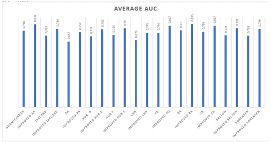
Figure 2. Average AUC of the algorithms.

According to the results of Figure 2, we notice that for all algorithms, the improved version has a higher AUC average than the existing metrics. For the preferential attachment metric, the improved AP is superior by $6.8\%$. We can draw the same conclusion for the rest of metrics.

The experiment shows that the proposed metric outperforms the existing local metrics. Furthermore, it demonstrates that any local metric may be improved in terms of precision. As expected, our metric gives a higher score to links in the $E_{test}$ against the links in $\overline{E}$. Then, the probability that a link exists in the graph G(V,E) is high compared to a link from $G(V,\overline{E})$. For instance, in the Power Grid dataset, LM has $AUC=0.59$ while the proposed weighted combination reached $AUC=0.73$.

From Figure 3, we can conclude that for the majority of datasets used to test the validity of our algorithm, the best $\alpha \in [0,5;1]$. Furthermore, we can notice that all the algorithms have the same $best$$\alpha$ for the same dataset, for instance, the $best\alpha$ is 0.9 for the YeastS network using all algorithms and 0.5 for all algorithms on Power Grid dataset. We then try to find a correlation between the $best\alpha$ and any network feature presented in Table 2.

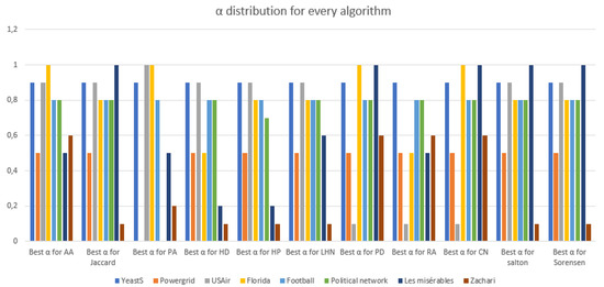
Figure 3. The $\alpha$ distribution on each dataset.

From Table 5 and using the rule of thumb, we can conclude that for AA and PA, we have a strong correlation between the $bestalpha$ and the average degree of the networks. For Jaccard, hub depressed, hub promoted, LHN and Sorensen, we have moderately strong correlation with r. For the metrics PD, CN and Salton, we have a moderately strong correlation with H. The RA index is the only metric to have a moderately strong correlation with C. Consequently, the parameter $\alpha$ can be written as a product of the network feature and a constant. For instance, $\alpha =average\_degree\times Constant$ for AA and PA.

Table 5. Correlation between the best $\alpha$ of each algorithm and the network features.

Correlation	Best $\mathit{\alpha }$ for AA	Best $\mathit{\alpha }$ for Jaccard	Best $\mathit{\alpha }$ for PA	Best $\mathit{\alpha }$ for HD	Best $\mathit{\alpha }$ for HP	Best $\mathit{\alpha }$ for LHN	Best $\mathit{\alpha }$ for PD	Best $\mathit{\alpha }$ for RA	Best $\mathit{\alpha }$ for CN	Best $\mathit{\alpha }$ for Salton	Best $\mathit{\alpha }$ for Sorensen
N	−0.347	−0.175	−0.328	0.097	0.052	−0.137	−0.183	0.113	−0.183	−0.183	−0.499
M	0.044	0.055	0.055	0.343	0.361	0.22	−0.12	0.1	−0.12	−0.12	0.055
C	0.034	0.143	0.123	−0.15	−0.209	−0.032	−0.229	−0.446	−0.229	−0.229	0.143
r	0.161	0.521	0.197	0.541	0.555	0.6	0.219	0.291	0.219	0.219	0.521
Average Degree	0.695	0.285	0.594	0.098	0.426	0.394	0.251	−0.237	0.251	0.251	0.285
D	−0.511	−0.277	−0.509	−0.048	−0.107	−0.218	−0.277	−0.078	−0.277	−0.277	−0.277
H	0.267	0.295	0.431	0.389	0.313	0.325	−0.547	−0.439	−0.547	−0.547	0.295
e	0.42	0.062	0.41	−0.234	−0.047	0.008	0.289	−0.124	0.289	0.289	0.062

5. Link Prediction Using Machine Learning Algorithms

In this section, we apply supervised learning algorithms to study the link prediction problem as a classification problem. We use random forest [40], k-nearest neighbors [41], support vector machine (SVM) [42], artificial neural network [43], and logistic regression [44]. Then, we compare the different supervised learning algorithms using the accuracy to evaluate their performance.

5.1. Methodology

To evaluate the performance of the proposed metric when modeling the link prediction as a classification task, we use the classification accuracy:

$$Accuracy=\frac{Numberofcorrectpredictions}{Totalnumberofpredictionsmade}$$

(15)

Let G(V, E) be an undirected and unweighted graph. In order to transform the link prediction problem into a binary task, we construct two sub-sets:

The first one contains the edges of E, the second one contains randomly chosen edges from $\overline{E}$. Then, we attribute a null value to the edges from $\overline{E}$ and 1 to those of E. We split them into test set and training set where the $testsize=10\%$. Finally, we train our classifier on the training set and then predict the test set. We use the Sklearn framework [45] to apply machine learning algorithms. Note that we use the best $\alpha$ of the improved RA for each dataset (see Figure 3).

5.2. Results

Table 6 shows the results of the KNN algorithm in two cases. The curve in blue represents the first case when we use only the state-of-the-art algorithms. The curve in orange represents the case in which we use the state-of-the-art algorithms along with the proposed metric. We can notice that the orange curve always has the highest accuracy, and we can conclude that the classification task becomes accurate when we add the PSI (Equation (13)) as an additional feature.

Table 6. The x axis represents the number of neighbors in the KNN model and the y axis is the accuracy.

Football dataset	Les Misérables dataset
Political Network dataset	Power Grid dataset
USAir dataset	YeastS dataset
Zachary dataset	Florida dataset

Table 7 shows the results of logistic regression. We obtain a higher orange curve when we apply PSI metric (Equation (13)) with the state-of-the-art algorithms as additional features of logistic regression. The curve in blue represents the case in which we only use the state-of-the-art algorithms. Note that for the Political Network, USAir and Zachary datasets, the logistic regression did not converge, and therefore we did not see a clear advantage.

Table 7. The x axis represents the inverse of regularization strength. The y axis is the accuracy of the logistic regression model.

Football dataset	Les Misérables dataset
Political Network dataset	Power Grid dataset
USAir dataset	YeastS dataset
Zachary dataset	Florida dataset

Table 8 shows the results of the random forest algorithm in two cases. We can notice that the orange curve has greater accuracy compared to the blue curve. Note that the curve in blue represents the first case in which we only use state-of-the-art algorithms. The curve in orange represents the case in which we use the state-of-the-art algorithms along with the proposed metric.

Table 8. The x axis represents the number of trees. The y axis represents the accuracy of the random forest model.

Football dataset	Les Misérables dataset
Political Network dataset	Power Grid dataset
USAir dataset	YeastS dataset
Zachary dataset	Florida dataset

Table 9 shows the importance of each feature used in the random forest algorithm (see Table 8). We can confirm that the proposed metric (Equation (13)) contributes more than the other metrics to the decision process.

Table 9. Random forest feature importances.

Football dataset	Les Misérables dataset
Political Network dataset	Power Grid dataset
USAir dataset	YeastS dataset
Zachary dataset	Florida dataset

Table 10 represents the weights of every hidden unit. The blue area represents large positive values, while the white area represents negative values. For every dataset, if the color of cells are darker, this means that the used parameter is important to the process. We notice that, for most of the datasets, our proposed metric has the darkest row. Thus, it plays a role in the decision-making process.

Table 10. Results of the neural network.

Football dataset
Les Misérables dataset
Political Network dataset
Power Grid dataset
USAir dataset
YeastS dataset
Zachary dataset
Florida dataset

From the Table 11, we can conclude that PSI (see Equation (13)) enhances the accuracy of KNN, especially for the Football, Power Grid and YeastS datasets. For the logistic regression algorithm, the best performance was for the Power Grid, Football, YeastS and Florida datasets. For the random forest model, we can notice that PSI enhanced the performance in all datasets; in addition, it further contributed to the decision process. We can draw the same conclusion for the neural network. Overall, decision tree has the best accuracy on all datasets. The results show that for all datasets, the performance increased when we used the PSI metric as an additional feature.

Table 11. Results of support vector machine (SVM), neural network and decision tree.

	Les Misérables	Political Network	Football	USAir	Power Grid	Zachary	Florida	YeastS
SVM with PSI	0.902	0.858	0.756	0.942	0.995	0.677	0.763	0.808
SVM without PSI	0.892	0.852	0.756	0.892	0.638	0.677	0.760	0.801
neural network with PSI	0.922	0.862	0.768	0.968	0.999	0.774	0.778	0.834
neural network without PSI	0.912	0.852	0.760	0.913	0.643	0.710	0.761	0.819
decision tree with PSI	0.971	0.875	0.959	0.969	0.998	0.903	0.740	0.985
decision tree without PSI	0.873	0.841	0.760	0.885	0.641	0.742	0.761	0.806

6. Conclusions

This paper presents a new parameterized metric for link prediction in social networks. We based the proposed metric on both mean received resources (MRRs) and a state-of-the-art local similarity measure (LM). The proposed metric is parameterized, and as a result, the system/user can adjust the importance of the factor under consideration. We tested the performance of the proposed metric using the AUC value on eight datasets from different fields, and we compared its results with 11 existing metrics.

The finding of this study shows that the proposed metric has a very high performance over the local similarity metrics in all datasets. It captures the interactions between unconnected nodes, even if they do not have common neighbors. Furthermore, we found a correlation between the parameter $\alpha$ and some networks’ features. In addition that, we used machine learning algorithms to classify links. The results show that whenever we use the proposed metric as an additional parameter, the accuracy of any algorithm increases; also, we concluded that the decision tree algorithm has the best performance in terms of accuracy.

This study can be extended to various networks such as directed networks, weighted networks. In addition, because most real-world networks are highly sparse, with a small number of positive cases relative to negative examples, dealing with imbalanced datasets in link prediction may be a real challenge.

References

- Esslimani, I.; Brun, A.; Boyer, A. Densifying a behavioral recommender system by social networks link prediction methods. Soc. Netw. Anal. Min. 2011, 1, 159–172. [Google Scholar] [CrossRef]
- Chen, H.; Li, X.; Huang, Z. Link prediction approach to collaborative filtering. In Proceedings of the 5th ACM/IEEE-CS Joint Conference on Digital Libraries (JCDL’05), Denver, CO, USA, 7–11 June 2005; IEEE: Piscataway, NJ, USA, 2005; pp. 141–142. [Google Scholar]
- Folino, F.; Pizzuti, C. Link prediction approaches for disease networks. In Proceedings of the International Conference on Information Technology in Bio-and Medical Informatics, Vienna, Austria, 4–5 September 2012; Springer: Berlin/Heidelberg, Germany, 2012; pp. 99–108. [Google Scholar]
- Wasserman, S.; Faust, K. Social Network Analysis: Methods and Applications; Cambridge University Press: Cambridge, UK, 1994. [Google Scholar]
- Aziz, F.; Cardoso, V.R.; Bravo-Merodio, L.; Russ, D.; Pendleton, S.C.; Williams, J.A.; Acharjee, A.; Gkoutos, G.V. Multimorbidity prediction using link prediction. Sci. Rep. 2021, 11, 16392. [Google Scholar] [CrossRef] [PubMed]
- Liben-Nowell, D.; Kleinberg, J. The link-prediction problem for social networks. J. Am. Soc. Inf. Sci. Technol. 2007, 58, 1019–1031. [Google Scholar] [CrossRef]
- Adamic, L.A.; Adar, E. Friends and neighbors on the web. Soc. Netw. 2003, 25, 211–230. [Google Scholar] [CrossRef]
- Jaccard, P. Étude comparative de la distribution florale dans une portion des Alpes et des Jura. Bull. Soc. Vaudoise Sci. Nat. 1901, 37, 547–579. [Google Scholar]
- Martínez, V.; Berzal, F.; Cubero, J.C. Adaptive degree penalization for link prediction. J. Comput. Sci. 2016, 13, 1–9. [Google Scholar] [CrossRef]
- Jibouni, A.; Lotfi, D.; El Marraki, M.; Hammouch, A. A novel parameter free approach for link prediction. In Proceedings of the 2018 6th International Conference on Wireless Networks and Mobile Communications (WINCOM), Marrakesh, Morocco, 16–19 October 2018; IEEE: Piscataway, NJ, USA, 2018; pp. 1–6. [Google Scholar]
- Ayoub, J.; Lotfi, D.; El Marraki, M.; Hammouch, A. Accurate link prediction method based on path length between a pair of unlinked nodes and their degree. Soc. Netw. Anal. Min. 2020, 10, 9. [Google Scholar] [CrossRef]
- Gu, S.; Chen, L. Link Prediction Based on Precision Optimization. In Proceedings of the International Conference on Geo-Informatics in Resource Management and Sustainable Ecosystem, Hong Kong, China, 18–20 November 2016; Springer: Berlin/Heidelberg, Germany, 2016; pp. 131–141. [Google Scholar]
- Han, S.; Xu, Y. Link Prediction in Microblog Network Using Supervised Learning with Multiple Features. J. Comput. 2016, 11, 72–82. [Google Scholar] [CrossRef][Green Version]
- Wang, Z.; Zhou, Y.; Hong, L.; Zou, Y.; Su, H. Pairwise Learning for Neural Link Prediction. arXiv 2021, arXiv:2112.02936. [Google Scholar]
- Matek, T.; Zebec, S.T. GitHub open source project recommendation system. arXiv 2016, arXiv:1602.02594. [Google Scholar]
- Ahmad, I.; Akhtar, M.U.; Noor, S.; Shahnaz, A. Missing link prediction using common neighbor and centrality based parameterized algorithm. Sci. Rep. 2020, 10, 1–9. [Google Scholar] [CrossRef] [PubMed]
- Kumar, A.; Singh, S.S.; Singh, K.; Biswas, B. Link prediction techniques, applications, and performance: A survey. Phys. Stat. Mech. Its Appl. 2020, 553, 124289. [Google Scholar] [CrossRef]
- Li, B.; Han, L. Distance weighted cosine similarity measure for text classification. In Proceedings of the International Conference on Intelligent Data Engineering and Automated Learning, Hefei, China, 20–23 October 2013; Springer: Berlin/Heidelberg, Germany, 2013; pp. 611–618. [Google Scholar]
- Barabâsi, A.L.; Jeong, H.; Néda, Z.; Ravasz, E.; Schubert, A.; Vicsek, T. Evolution of the social network of scientific collaborations. Phys. Stat. Mech. Its Appl. 2002, 311, 590–614. [Google Scholar] [CrossRef]
- Newman, M.E. Clustering and preferential attachment in growing networks. Phys. Rev. E 2001, 64, 025102. [Google Scholar] [CrossRef] [PubMed]
- Ravasz, E.; Somera, A.L.; Mongru, D.A.; Oltvai, Z.N.; Barabási, A.L. Hierarchical organization of modularity in metabolic networks. Science 2002, 297, 1551–1555. [Google Scholar] [CrossRef]
- Leicht, E.A.; Holme, P.; Newman, M.E. Vertex similarity in networks. Phys. Rev. E 2006, 73, 026120. [Google Scholar] [CrossRef]
- Zhu, Y.X.; Lü, L.; Zhang, Q.M.; Zhou, T. Uncovering missing links with cold ends. Phys. Stat. Mech. Its Appl. 2012, 391, 5769–5778. [Google Scholar] [CrossRef]
- Salton, G.; Mcgill, M. Introduction to Modern Information Retrieval; McGraw-Hill, Inc.: New York, NY, USA, 1986; 400p. [Google Scholar]
- Sorensen, T.A. A method of establishing groups of equal amplitude in plant sociology based on similarity of species content and its application to analyses of the vegetation on Danish commons. Biol. Skar. 1948, 5, 1–34. [Google Scholar]
- Zhou, T.; Lü, L.; Zhang, Y.C. Predicting missing links via local information. Eur. Phys. J. B 2009, 71, 623–630. [Google Scholar] [CrossRef]
- Fishburn, P.C. Letter to the editor—Additive utilities with incomplete product sets: Application to priorities and assignments. Oper. Res. 1967, 15, 537–542. [Google Scholar] [CrossRef]
- Han, J.; Moraga, C. The influence of the sigmoid function parameters on the speed of backpropagation learning. In Proceedings of the International Workshop on Artificial Neural Networks, Perth, Australia, 27 November–1 December 1995; Springer: Berlin/Heidelberg, Germany, 1995; pp. 195–201. [Google Scholar]
- Bu, D.; Zhao, Y.; Cai, L.; Xue, H.; Zhu, X.; Lu, H.; Zhang, J.; Sun, S.; Ling, L.; Zhang, N.; et al. Topological structure analysis of the protein–protein interaction network in budding yeast. Nucleic Acids Res. 2003, 31, 2443–2450. [Google Scholar] [CrossRef] [PubMed]
- Nakai, K.; Kanehisa, M. Expert system for predicting protein localization sites in Gram negative bacteria. Proteins Struct. Funct. Bioinform. 1991, 11, 95–110. [Google Scholar] [CrossRef]
- Kunegis, J. Konect: The koblenz network collection. In Proceedings of the 22nd International Conference on World Wide Web, Rio de Janeiro, Brazil, 13–17 May 2013; pp. 1343–1350. [Google Scholar]
- Watts, D.J.; Strogatz, S.H. Collective dynamics of ’small-world’networks. Nature 1998, 393, 440–442. [Google Scholar] [CrossRef] [PubMed]
- Batagelj, V.; Mrvar, A. Pajek Datasets. USAir97. Net. 2006. Available online: http://vlado.fmf.uni-lj.si/pub/networks/data/ (accessed on 10 November 2021).
- Ulanowicz, R.E.; DeAngelis, D.L. Network analysis of trophic dynamics in south florida ecosystems. Geol. Surv. Program South Fla. Ecosyst. 2005, 114, 45. [Google Scholar]
- Girvan, M.; Newman, M.E. Community structure in social and biological networks. Proc. Natl. Acad. Sci. USA 2002, 99, 7821–7826. [Google Scholar] [CrossRef]
- Rossi, R.; Ahmed, N. The network data repository with interactive graph analytics and visualization. In Proceedings of the Twenty-Ninth AAAI Conference on Artificial Intelligence, Austin, TX, USA, 25–30 January 2015. [Google Scholar]
- Latora, V.; Marchiori, M. Efficient behavior of small-world networks. Phys. Rev. Lett. 2001, 87, 198701. [Google Scholar] [CrossRef]
- Newman, M.E. Assortative mixing in networks. Phys. Rev. Lett. 2002, 89, 208701. [Google Scholar] [CrossRef]
- Snijders, T.A. The degree variance: An index of graph heterogeneity. Soc. Netw. 1981, 3, 163–174. [Google Scholar] [CrossRef]
- Breiman, L. Random forests. Mach. Learn. 2001, 45, 5–32. [Google Scholar] [CrossRef]
- Goldberger, J.; Hinton, G.E.; Roweis, S.; Salakhutdinov, R.R. Neighbourhood components analysis. Adv. Neural Inf. Process. Syst. 2004. Available online: https://citeseerx.ist.psu.edu/viewdoc/download?doi=10.1.1.449.1850&rep=rep1&type=pdf (accessed on 10 November 2021).
- Wu, T.F.; Lin, C.J.; Weng, R.C. Probability estimates for multi-class classification by pairwise coupling. J. Mach. Learn. Res. 2004, 5, 975–1005. [Google Scholar]
- Hkdh, B. Neural networks in materials science. ISIJ Int. 1999, 39, 966–979. [Google Scholar]
- Kleinbaum, D.G.; Dietz, K.; Gail, M.; Klein, M.; Klein, M. Logistic Regression; Springer: Berlin/Heidelberg, Germany, 2002. [Google Scholar]
- Pedregosa, F.; Varoquaux, G.; Gramfort, A.; Michel, V.; Thirion, B.; Grisel, O.; Blondel, M.; Prettenhofer, P.; Weiss, R.; Dubourg, V.; et al. Scikit-learn: Machine Learning in Python. J. Mach. Learn. Res. 2011, 12, 2825–2830. [Google Scholar]
Publisher’s Note: MDPI stays neutral with regard to jurisdictional claims in published maps and institutional affiliations. |
© 2022 by the authors. Licensee MDPI, Basel, Switzerland. This article is an open access article distributed under the terms and conditions of the Creative Commons Attribution (CC BY) license (https://creativecommons.org/licenses/by/4.0/).