Abstract
Conventional approaches to modelling driver risk have incorporated measures such as driver gender, age, place of residence, vehicle model, and annual miles driven. However, in the last decade, research has shown that assessing a driver’s crash risk based on these variables does not go far enough—especially as advanced technology changes today’s vehicles, as well as the role and behavior of the driver. There is growing recognition that actual driver usage patterns and driving behavior, when it can be properly captured in modelling risk, offers higher accuracy and more individually tailored projections. However, several challenges make this difficult. These challenges include accessing the right types of data, dealing with high-dimensional data, and identifying the underlying structure of the variance in driving behavior. There is also the challenge of how to identify key variables for detecting and predicting risk, and how to combine them in predictive algorithms. This paper proposes a systematic feature extraction and selection framework for building Comprehensive Driver Profiles that serves as a foundation for driver behavior analysis and building whole driver profiles. Features are extracted from raw data using statistical feature extraction techniques, and a hybrid feature selection algorithm is used to select the best driver profile feature set based on outcomes of interest such as crash risk. It can give rise to individualized detection and prediction of risk, and can also be used to identify types of drivers who exhibit similar patterns of driving and vehicle/technology usage. The developed framework is applied to a naturalistic driving dataset—NEST, derived from the larger SHRP2 naturalistic driving study to illustrate the types of information about driver behavior that can be harnessed—as well as some of the important applications that can be derived from it.
1. Introduction
Driver profiles are commonly defined as profiles that represent the overall characteristics of a driver, which can include multiple driver traits such as demographics, personality, and lifestyle; and driving behaviors such as on- and off-road glances, secondary driving tasks, technology usage associated with the vehicle; as well as personal electronics carried into the vehicle [1]. A driver profile is different from driving behavior profiles, driving style profiles, and driver types. Driving behavior profiles are descriptions of different behavioral characterization processes where the approach focuses on behavior classification. Driving behavior profiles can be composed of behaviors ranging from few to many, and may or may not reflect the entire observed variability across a representative sample of a driver’s trips [2]. Driving styles represent a stable aspect of driving behavior, and refer to the habitual way of driving, which is characteristic for a driver or a group of drivers [3]. Whereas driver types, often used interchangeably with driving styles, refer to driving behaviors that represent a stable personality trait [4]. From a hierarchy perspective, driving styles and types are considered subcategories of driving behavior profiles, and driving behavior profiles are considered building blocks of a driver profile [2,3].
A major drawback for building driver profiles is the lack of a consensus on the set of driver characteristics and behaviors that are considered consistently useful in developing reliable and representative profiles of the driver relative to the outcome of interest. For example, in naturalistic driving studies, there has been a concerted effort to build profiles specifically related to a driver’s crash risk. Early studies showed that the most important behaviors associated with predicting risk were measures of speeding, acceleration, braking events, and lane changing [5,6,7]. However, recent studies have suggested that along with these measures, temporal factors such as time of day, and spatial factors such as speed limit and weather conditions are also strong predictors of crash risk, and should be included in a driver’s profile model [8]. Other studies have found that factors such as lead vehicle following distance, braking response time, driver experience and exposure, along with non-driving behaviors such as alcohol consumption, socioeconomic, psychological, and lifestyle also influence a driver’s behavior, and thus, are also important for building more complete driver risk profiles [9,10,11,12]. In all these studies, the most valuable conclusion is that while at least five predictors are often needed for building driver risk profiles; the predictors are not always the same, and the degree to which the unique predictors relate to crash risk are not consistently significant.
To address the challenge of building reliable and whole driver profile models, studies have turned to machine learning (ML) algorithms. Several ML algorithms such as fuzzy control theory, Dynamic Time Warping, artificial neural networks (ANN), support vector machines (SVM), and Bayesian Networks have been used to build driver profiles using a wide range of driving behaviors [13]. These ML algorithms are powerful and widely used in designing intelligent driver identification, support, and safety systems because they demonstrate high accuracies for driver classification [14,15]. Despite these approaches offering robust processing, above average classification, and a high rejection ratio for noise, they come with their own set of challenges.
A major challenge when applying ML algorithms toward driver profiling and identification is the complexity involved in extracting the underlying models. ML algorithms are not all black boxes, but understanding the underlying model architecture, hyperparameters, and decision boundaries that relate the accuracy of the driver identification models to driving behaviors and context is complex. While reverse engineering these ML algorithms has gained traction [16], and can be implemented to extract the main effects of many of these approaches, it is impossible to test for all the interaction effects, wherein lie the unknown elements that influence the underlying model behavior. Thus, while ML algorithms provide high accuracy, their high degree of complexity makes it challenging to interpret the model outcomes, and relate them back to the driver as useful feedback.
Developing comprehensive driver profiles with high accuracy is a goal that can be obtained at the level desired without requiring the use of ML algorithms that have a high degree of complexity. While there have been a number of notable studies that have reportedly developed reliable driver scoring and profiling metrics for crash risk prediction, driver distraction, etc., these efforts, despite using complex ML algorithms, have not established driver profiles that incorporate a wide range of driving behaviors and driving contexts [17]. Instead, they have used only three to four variables to develop driver profiles, and have suggested that the frameworks can be extended to encompass more variables [2].
With the growing availability of large naturalistic driving datasets, there is an acute need for an approach to build reliable driver profiles that are capable of synthesizing as much of the salient data as possible into meaningful profiles and useful generalizations without using complex ML algorithms. While ML approaches with feature selection techniques have been implemented to compress large naturalistic driving study (NDS) datasets to find the most informative driving behavior and driver profile, few studies have focused on the intersection of feature extraction and feature selection from NDS datasets for building whole and comprehensive driver profiles. This paper proposes a systematic feature extraction and selection framework for building Comprehensive Driver Profiles (CDPs) that serve as a foundation for driver behavior analysis and building whole driver profiles. The proposed Comprehensive Driver Profile framework is applied to an NDS dataset NEST, to demonstrate the importance of a systematic feature extraction and selection process, and to provide examples on the usefulness and insights that can be extracted from building such comprehensive driver profiles that can provide opportunities for personalizing HMI design and application, driver identification, driver behavior profiling, driver behavior modification programs, and usage-based insurance (Pay-How-You-Drive).
2. A Framework for Building Comprehensive Driver Profiles
In this section, a methodology for building Comprehensive Driver Profiles (CDPs) is outlined. Under this framework, Comprehensive Driver Profiles (CDPs) are defined as the minimum set of features that identify and represent a driver within a specified degree of accuracy for an outcome of interest such as risk, attention, distraction, etc. Within this definition, features are simply variables representing observable phenomena that can be quantified and recorded, or derived properties of instances in a model’s domain. Whereas accuracy refers to model accuracy, which is the measurement used to determine which model is best at identifying relationships and patterns between features in a dataset. The better a model can generalize to ‘unseen’ data, the better detection, prediction, and insights it can produce.
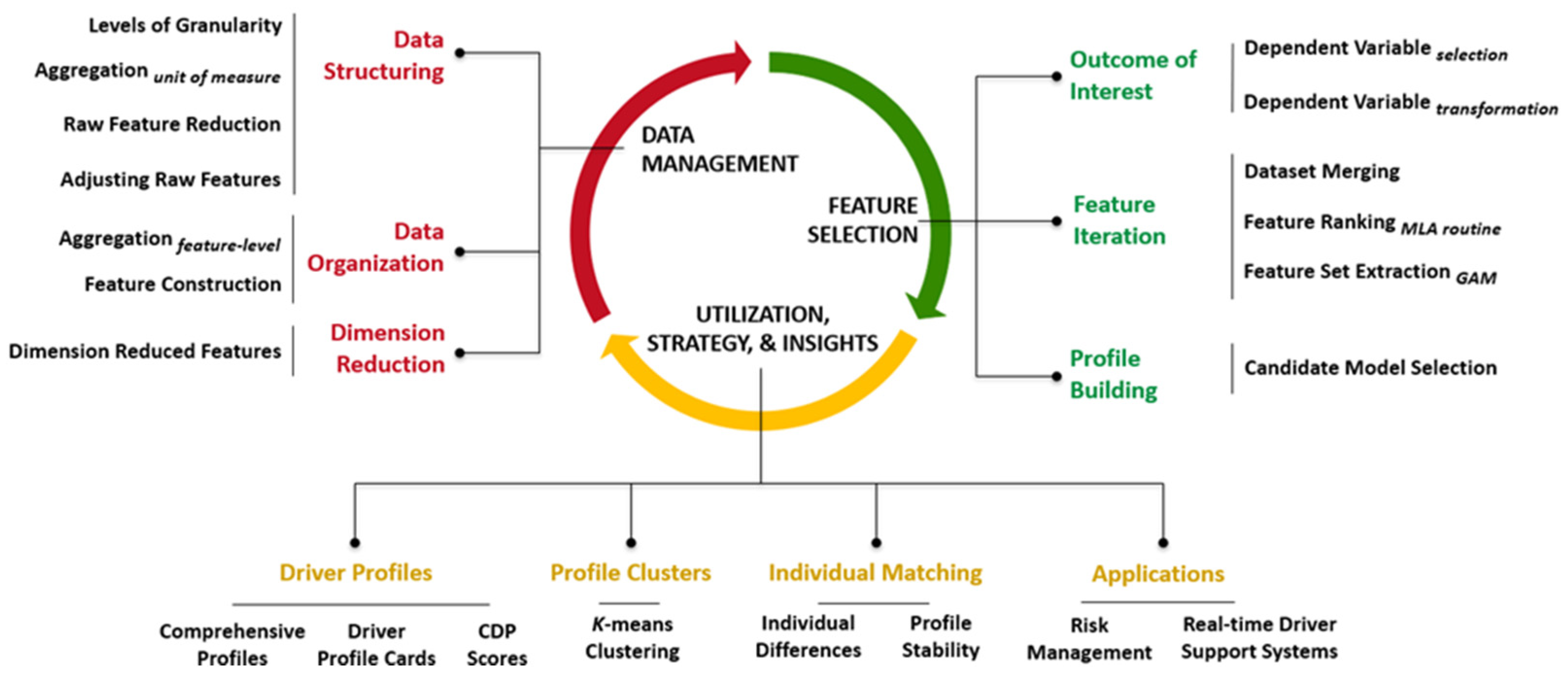
The framework for building Comprehensive Driver Profiles (CDPs) consists of three stages: Data Management, Feature Selection, and Utilization, Strategy, and Insights (Figure 1). The Data Management stage provides guidelines for structuring and organizing the data so that it can be appropriately implemented for dimension reduction before the CDPs are built. The Feature Selection stage is used to select the relevant features for driver profile model construction using an iterative approach. Additionally, the Utilization, Strategy, and Insights stage provides a suite of approaches to compare the CDPs both at the population as well as individual level, and garner insights that have applications toward customizable driver support system feedback and risk management. The cyclical nature of the framework allows the driver profiles to be constantly updated as more trips are driven and more behaviors and context are recorded. This enables continuous improvement of the CDPs by monitoring when there is a dramatic change in one or more driver profiles, and identifying what behaviors and driving context had an effect. The following sections detail the methodology of the framework, with relevant examples of how to implement the CDP framework on datasets such as NEST (Naturalistic Engagement in Secondary Tasks) as an illustration.

Figure 1.
Framework for building whole and comprehensive driver profiles (CDPs).
2.1. Naturalistic Engagement in Secondary Tasks (NEST) Dataset
The Naturalistic Engagement in Secondary Tasks (NEST) dataset is used to illustrate the steps of the CDP framework for the purpose of developing comprehensive driver crash risk profiles. NEST is a dataset from drivers who experienced a safety critical event (SCE) with secondary task activity as a contributing factor and contains crash-involved drivers. The dataset does not contain drivers that did not experience a secondary task-related SCE. The NEST dataset is used only as an example in this paper to show how large naturalistic driving datasets can be analyzed using the proposed CDP framework. Therefore, issues and complexities associated with using the NEST dataset—such as the fixed set of randomly selected baselines (drawn from separate trips of the drivers—which might result in biased exposure rates, or derivation of EDKs without video-validation, etc.—are not addressed).
The NEST dataset consists of naturalistic data for 204 drivers that were drawn from full trips that ended in a distraction-related crash. The NEST dataset was created to provide the research community with a dataset tailored for the study of secondary task engagement and its role in distraction and crash risk—and contains data from epochs of driving that immediately preceded crash, as well as baseline epochs (free from safety-critical events) that could be used for comparison [18]. NEST is a subset of the SHRP2 dataset [19,20], created by Virginia Tech Transportation Institute (VTTI) under funding from the Toyota Collaborative Safety Research Center (CSRC). Thus, NEST consists of epoch-based data, with 236 SCE epochs and four baseline driving epochs for each driver who contributed an SCE epoch. For all the SCE epochs, continuous frame-by-frame coding of glances, secondary task activities, and hands-on/off wheel activity was available for 20 s before the crash occurred from the precipitating event, and extended forward from the precipitating event for 10 s after. Thus, each SCE epoch in NEST is 30 s long, with matched lengths of comparison baseline driving epochs for each driver.
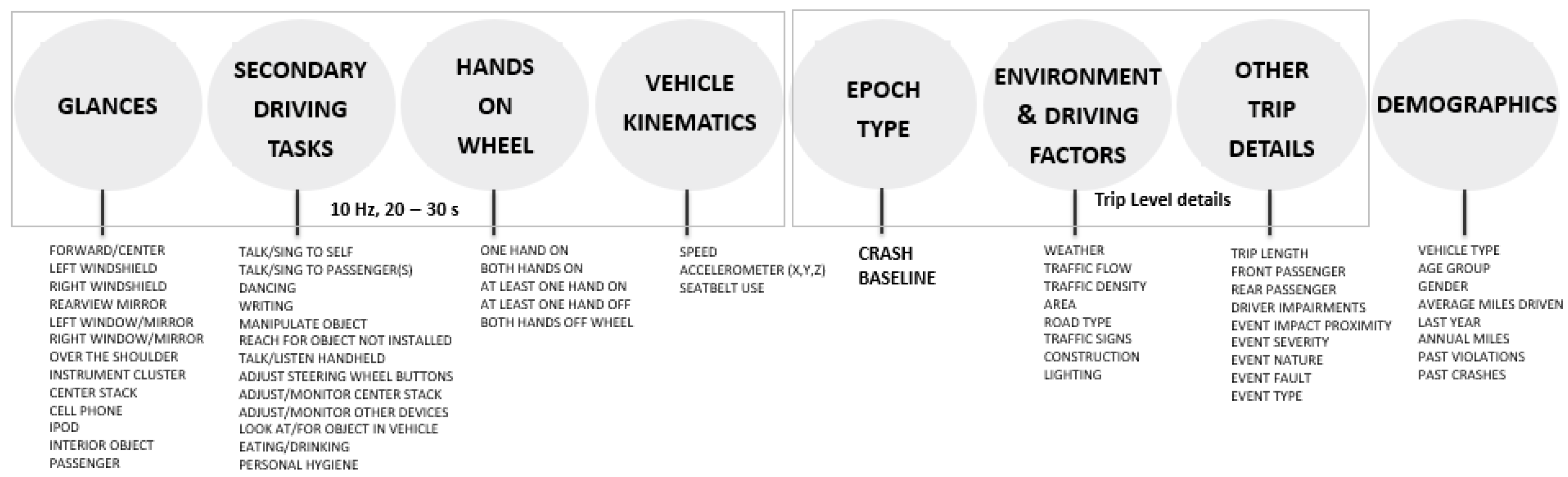
In NEST, speed, glances, secondary task activity, and hands-on/off wheel variables were available at the 10 Hz rate for the 30 s epochs. Whereas environment and driving factors, along with other trip and crash event details were coded periodically at 10 s intervals within the 30 s epochs. Crashes were classified as an event if there was any contact between the subject vehicle and an object, either moving or fixed, at any speed, in which kinetic energy was measurably transferred or dissipated. Additionally, glances in the NEST dataset were assessed as the proportion of time within the epoch that the driver’s eyes were directed to a given glance location. All the NEST variables used for implementing the CDP framework are shown in Figure 2. Detailed review of the dataset and definitions of each of the variables can be found in [18].
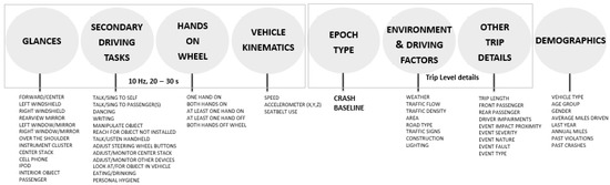
Figure 2.
Variables in the Naturalistic Engagement in Secondary Tasks (NEST) dataset used for implementing the steps of the CDP framework.
2.2. CDP Step 1: Data Management
The Data Management stage involves three main steps: data structuring, data organization, and dimension reduction (Figure 1) that serve as guidelines for data setup prior to feature selection. The data structuring process involves organizing the data into matrices to reflect the different levels of granularity. For the NEST dataset, the matrices that represent different levels of granularity are denoted as , , and datasets (Table 1) where the segment level ( dataset) refers to matrices where only parts of a trip are available such as epochs.

Table 1.
Example of matrices built for different levels of granularity: sample, segment, trip, and driver.
Determining the level of aggregation is an important next step. At the sample level, aggregation is performed with respect to the unit of measure. A very granular unit of measure at the sample level will result in computational issues and diminish the ability to capture relevant information to assess the driving situation. Whereas highly aggregated data will afford computational ease but can suffer from loss of quality of information [21]. Additionally, highly aggregated data reduce variation and updates very slowly, making it less reliable for real-time application. For datasets similar in structure to NEST, aggregation between 1–3 s is preferred for implementing the framework. Thus, the NEST dataset was assessed at the sample level and aggregated to 1 s.
After aggregation, the number of raw features were reduced and adjusted. In NEST, raw features were removed if they had no relationship with driving-related outcomes, and if features had perfect or near perfect collinearity. Since many of the methods leveraged for creating profiles require quantitative features, adjustments to any of the qualitative (categorical) features were also made.
One of the goals of the CDP framework is to limit the amount of manual processing of the data. Manual processing involves using heuristic knowledge and ad-hoc data analysis to reduce raw features of the data before any modelling. Most of the driver profile frameworks in the literature conduct manual processing to filter out unrepresentative data. With datasets of high-dimensionality, there is a need for raw feature reduction to make modelling feasible. Too many raw features, especially if loosely related to the driving outcomes, will increase type II error rates and vastly increase computation time.
An important step for creating meaningful driver profiles is leveraging the raw data to create features. Feature construction approaches involve variables that are aggregated, lagged, have memory, and other types of feature derivations. While a number of features can be created, for illustration purposes, only aggregated features are detailed in this section. Aggregated features are from datasets that vary with time, but can also arise from features that vary by a qualitative category. Focusing on time first and starting with the most granular time-varying dataset is the easiest method to follow. Each feature within the sample level data has two metrics derived from it: the mean and standard deviation. These metrics are obtained at each level of increasing granularity, from segment level to the driver level (1).
In (1), is the th feature in the sample level data, and , , and are the corresponding segment, trip, and driver key identification references associated with each of the rows. Each of the features in the sample level dataset will now have a mean aggregated feature (MAF) at the segment level, which in turn can be joined into the segment level data . This step can also be repeated for the standard deviation, creating standard deviation aggregated features (STAF) (2). The MAFs and STAFs are then joined into the driver level dataset, .
After conducting the time aggregation, other aggregates based on categorical features are created in a similar manner. For NEST, the action was performed at the epoch (segment) level as it is the next level of granularity after the sample level. In NEST, a key categorical variable used at the epoch level was whether the recorded epoch was a baseline or crash epoch. Along with the aggregated features, features were also lagged by 1 s and 2 s. Thus, the final NEST dataset () consisted of aggregated and lagged variables.
The last step in the Data Management stage is dimension reduction. Dimension reduction algorithms are used to obtain compact, accurate representations of multivariate data by maintaining the breadth of information. These algorithms help reduce noise by eliminating statistically redundant components, thereby creating a better platform for interpreting a large number of features [22,23]. While there are a number of dimension reduction techniques such as t-SNE and Isomap that can be implemented, the approach recommended for building CDPs is Principal Component Analysis (PCA) because it allows reconstruction of the original features.
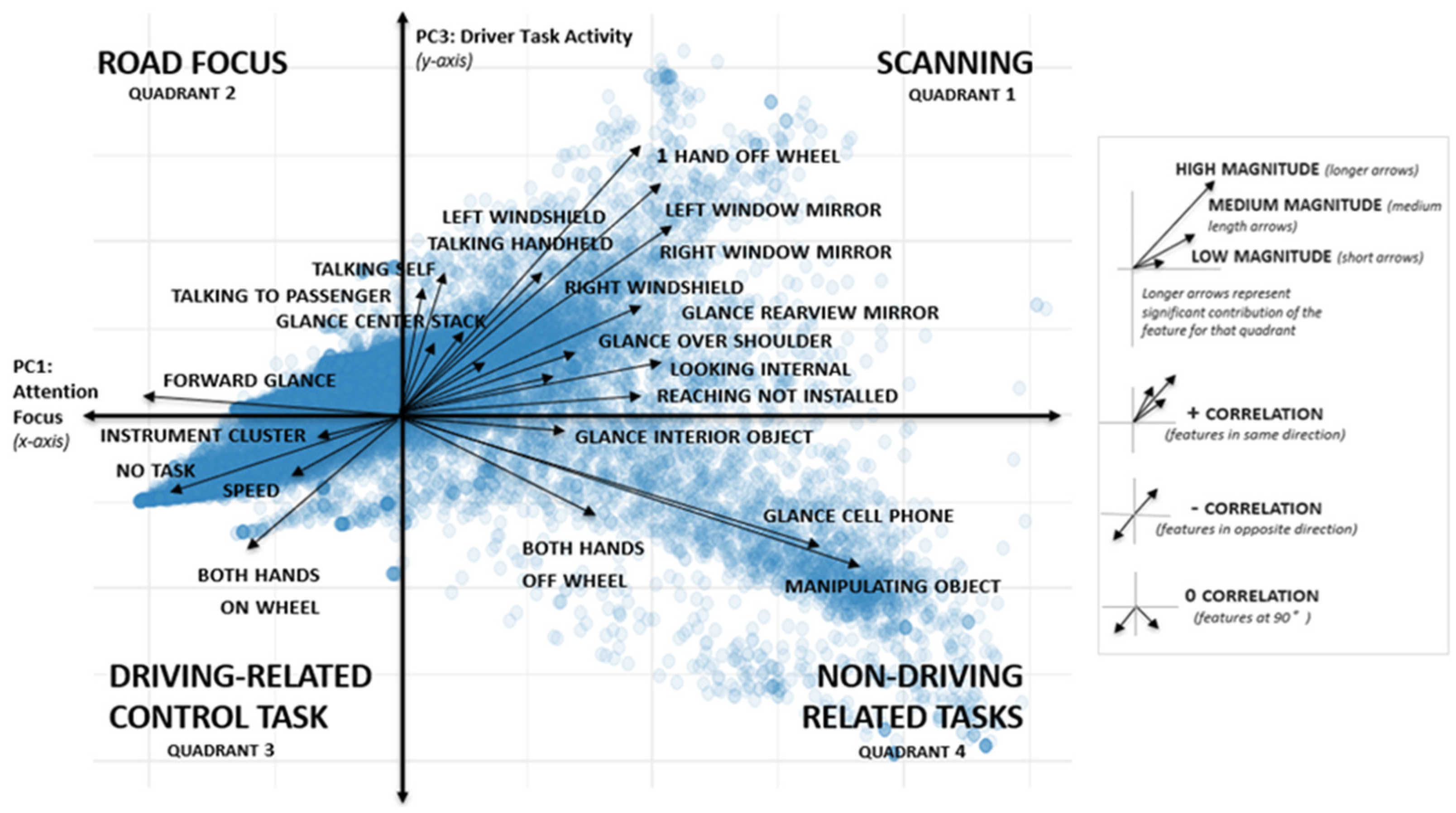
PCA is an unsupervised dimension reduction approach that allows mapping of data from a high-dimensional space to a low-dimensional space while retaining the relevant data structure [21]. PCA was applied to dataset , which consisted of 141 features (Table 2). Results from the PCA produced principal components (PC), where the first component PC1 accounted for 22% of the total variance, followed by PC2 and PC3 with variances of 19% and 15%, respectively. An inspection of the features within each of the PCs revealed that PC1 and PC3 produced the most interpretable results related to the outcome of interest–crash risk (Figure 3).
Table 2.
Principal component analysis (PCA) on the NEST dataset.
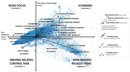
Figure 3.
Framework for building whole and comprehensive driver profiles (CDPs).
Figure 3 shows the distribution of the features that had the strongest contributions to PC1 and PC3. In Figure 3, features along PC1 (horizontal axis) and PC3 (vertical axis) were interpreted to represent ‘attentional focus’ and ’type of driver task activity’, respectively. PC1 and PC3 also divided the PCA plot into four interpretable quadrants, where features in each quadrant were positively correlated (Table 3). Results from the PCA successfully provide an insightful assessment of the structure of the NEST data. For example, Figure 3 shows that when NEST drivers were primarily conducting scanning behaviors and glances (quadrant 1), they were less likely to be driving at higher speeds (quadrant 3). Whereas when drivers were primarily focused on the road (quadrant 2), they were less likely to be conducting non-driving related tasks such as using their phone (quadrant 4).
Table 3.
PCA results: description of the 4 quadrants.
2.3. CDP Step 2: Feature Selection
The Feature Selection stage involves three main steps: selecting the outcome of interest, profile feature iteration, and building CDPs (Figure 2). The goal of the Feature Selection stage is to eliminate features that are irrelevant or redundant for building profiles for the outcome of interest. The advantages of conducting feature selection at this stage are that it reduces the computational costs associated with high-dimensional data that would otherwise be required to extract features; makes it easier to relate the reduced feature set for profile building to the outcome of interest [24], and reduce over-fitting [22].
In NEST, the risk of crashing was selected as the outcome of interest. The fact that an epoch was a crash was encoded at the sample level (in the variable called ‘Epoch Type’ shown in Figure 2). This means that for each second of driving, the probability of a crash in that same second was computed. Each second of the sample level consisted of 10 samples aggregated into a single value. To determine crash instances, each second was scored by how many 100 ms samples within that second occurred during the actual crash event itself, and was represented fractionally as a proportion between 0 and 1. Since the goal of this paper is to provide an example of how to implement the CDP framework on datasets such as NEST, the central focus is not on the fraction of time that contained the crash but on whether a crash occurred. Therefore, each second of driving that contained any portion of a crash event was rounded up to 1, creating a binary indicator of whether a crash occurred or not. This enables the setup for any basic ML algorithm to determine the probability of a crash using common classification and binary outcome routines [22].
A tenet of the CDP framework is the notion that for driver profiles to be comprehensive, they should be feature-complete. Thus, feature iteration in the CDP framework is conducted to obtain feature-complete driver profiles, where feature-complete is defined as the minimum set of features necessary to explain or predict a driving-related outcome of interest with a desired degree of accuracy. Before addressing considerations for the accuracy threshold, it is important to first establish the goal of developing CDPs. If CDPs are needed for real-time assessment of a potential crash or safety-critical event, then prediction is the preferred metric to set for feature-complete. Conversely, if the profiles are for long-term planning, strategy, or post-trip driver feedback; then detection would likely be the preferred metric set for feature-complete. In this paper, the illustration of the CDP framework using NEST is focused on long-term planning and strategy around a driver’s crash risk. Hence, detection (explanation) of crash incidents is used instead of prediction as the outcome of interest.
To establish an appropriate measure of accuracy for the feature-complete driver profiles, an a priori desired degree of accuracy was defined to be an Area Under the Receiver Operating Characteristic Curve (AUC) of 75%. Here, AUC is a measure of the ability of the profile to differentiate between a crash and non-crash driving event [23]. Prior to conducting the feature iteration step, datasets , , , and are merged to create a modeling dataset, on which to obtain the features that satisfy the criteria for feature-complete profiles. Modeling is conducted at the sample level because detection of crashes is used as the outcome of interest.
To reduce over-fitting and to check for robustness, the dataset (features = 120, which includes glance and behavior PCA features) was split into training () and test () datasets, with the test comprised of 20% of the data. Random Forest (RF) was used to find the minimum set of features involved by conducting a pre-screening of variables [25,26]. Although literature on RF depicts and treats it as a black box, node analysis can be conducted on the decision paths in RF, to extract and understand the underlying interaction effects and individual decisions that contribute to the final outcome. The use of RF in the CDP framework to compute feature importance makes the framework versatile because RF can be applied to a wide range of prediction problems, even if they are nonlinear, and involve complex high-order interaction effects, which makes it highly applicable for naturalistic driving data [27].
For the Feature Selection stage, permutation was considered the most appropriate importance measure for running RF [25]. The permutation feature importance measure is a model inspection technique that is used to determine the decrease in model score when a single feature is randomly shuffled [28]. This technique breaks the relationship between the feature and the target. Additionally, the change in the model score represents how much the model depends on the feature. For the dataset , RF was run using the R Ranger package [29]. For the RF analysis, the number of trees were 1500, the number of variables to sample at each split was set to be the square root of the number of columns in dataset X, and the minimum node size was 6. The importance method was set to be ‘permutation’, and the scale permutation importance factor was set to ‘false’. Results of the RF are shown in Table 4. These results were used to determine the number of necessary variables for constructing interpretable feature-complete driver risk profiles.
Table 4.
Random forest importance table. Any feature with a relative importance < 0.015 was removed from consideration for building the profiles. Only the top 10 features are shown in this table.
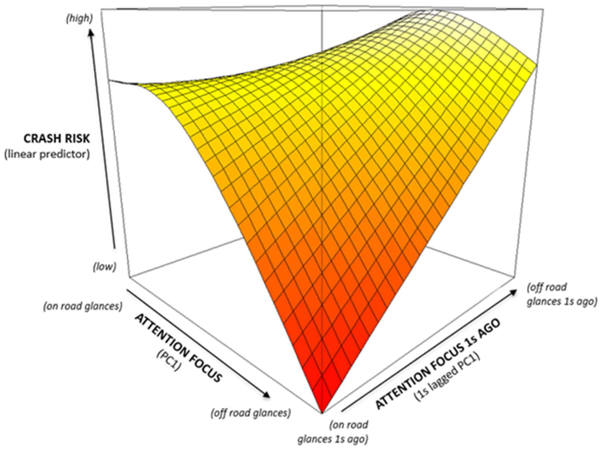
Before extracting the feature-complete set for building driver profiles, some statistical analyses, data visualizations, and goodness of fit analyses were conducted on the RF model output. Visual analyses and preliminary models using the top features from the model output (Table 4) were built using a class of regression models—Generalized Additive Models (GAMs) [30]. GAMs are a type of regression that specializes in estimating non-linear effects, and are unique in their flexibility to estimate unbiased effects [30]. For the NEST dataset, assessment on the importance table output (Table 4) of the RF model revealed a high degree of interaction between the top features and their effect on crash detection. An example of this type of interaction is shown in Figure 4. In Figure 4, the top of the cube is associated with higher crash risk, and the bottom of the cube with lower crash risk. The axes PC1 and lagged PC1 represent the principal component loading from the PCA analyses that is associated with glances on and off the road and their respective 1 s lags, whereas the axis representing the linear predictor is the risk of crashing.

Figure 4.
Example of the interaction effects between the driving glances and behaviors in the NEST data.
In Figure 4, higher values (direction of the arrow along each axis) indicate attention being diverted from the road. The interaction effect shows low risk at the near and far corners, and higher risk at the left and right corners, and along the ridge in between them. This suggests that risk increases when the glance location remains fixed, and decreases when it moves around. This is true even when there is a large amount of attention away from the road in the current second, which means that as long as attention returns to the road within the next second, much of the risk is averted. It is interesting to note that this is also true for staring only at the road (top left corner in Figure 4), suggesting that an element of ‘zoning-out’ on the road (possibly capturing mind wandering) is associated with a higher risk of crashing. These effects were pervasive in many of the glance and behavior PCA features. Hence the next step uses these features to build the baseline model for profile building. Since the goal of this paper is to demonstrate the CDP framework methodology, the interpretation of results for each process of the CDP framework using NEST is limited to maintain the scope of this paper.
Starting from the baseline model (Equation (3)) and using the RF importance scoring—a forward and backward stepwise regression method was used for adding variables [31]. A list of candidate models was set aside, to be used in the final cross-validation on . It is important to build a complete set of candidate models before attempting any cross-validation on the test set, as this helps reduce over-fitting and data mining, thereby reducing the chance of building driver profiles that do not generalize well [32]. For the development of the driver profile models using the NEST dataset, nine candidate models were created during the forward and backward stepwise model building process. These models were selected based on goodness of fit measures: adjusted R-squared and generalized cross-validation criterion. In Equation (3), te() refers to a tensor plate spline method used in GAM [30].
It should be noted that the number of candidate models is not of vital importance, especially if they are derived from the method outlined above. More important is that the models have some variation between them in how they describe the outcome of interest, i.e., they do not share too many of the same features and have a varying number of features. To account for additional type II error rates when using a set of candidate models, the Bonferroni correction was applied for significance testing [33]. The full setup for the NEST feature-complete model testing requirements is shown in Table 5. In Table 5, the selected criteria for success AUC ≥ 0.75 means that for the driver profiles to be ‘useful’ or for detection to be considered ‘successful’, the profile has to have at least a 75% chance of ranking a segment of driving with a crash higher than one without a crash, and that the approach will determine a profile with this property at least 95% of the time. With this information criteria, cost-benefit decisions can be made on how to employ the profiles, and what the expected benefits will be once these profiles are applied.
Table 5.
Feature-complete model testing requirements.
Values in Table 5 provide an example of how to evaluate whether there exists a profile that meets the a priori expectations of a useful profile. Users of the profiles (e.g., insurance and car companies) can determine these values based on the intended application and risk-to-benefit ratios. Table 5 also illuminates that Power testing should be conducted when determining the desired values and significance thresholds. For NEST, had a crash prevalence of 1.29% ( ( = 154), ( = 11,765)). These data can be used to evaluate the expected power of the profiles on as shown in (Equation (4)).
The null hypothesis based on Table 5,
Using standard Z-test methods, this gives rise to the following rejection region,
Application of these methods produced the following power values (Table 6). The first column shows the dilemma faced: If a low chance of choosing a model with AUC is less than 0.75, there will be less than a 50% chance of accepting a model even if the true AUC is as high as 0.85. The second column again shows a more prudent route, where lowering the minimum acceptable model to 0.70 and relaxing the significance requirement gives at least a chance of accepting models that are as good as or better than the ideal profile.
Table 6.
Power table for acceptable profile models.
The results in Table 7 on the NEST crash risk driver profiles allows appropriate grading of the output of the nine candidate models, with the highlighted row identifying the model that satisfied the criteria of minimum set of features that described crashes with an AUC of at least 0.70. Although there are better models from an observed AUC perspective, since they have more features, they were passed over in favor of the qualifying model with the least number of features. This adheres to the notion that a choice can be made deeming performance above the threshold unnecessary, and the trade-off of more succinct and leverageable profiles preferred.
Table 7.
Ability of the nine candidate driver profile models to distinguish crash vs. no-crash epochs. The winning GAM candidate model that best satisfied the feature-complete requirements consisted of 8 features—model rank 4.
The winning GAM candidate model (Table 7) that best satisfied the feature-complete requirements consisted of eight features (Equation (5)). The GAM model results are shown in Table 8. Because the dependent variable is the probability of a crash in the current 1 s window, positive coefficients in the model (Table 8) indicate that an increase in the features are associated with increased crash risk, and vice-versa. An interesting finding from Table 8 is that driving in heavier traffic and rain both increased the risk of a crash by nearly equivalent amounts (odds increase by ).
Table 8.
Winning candidate model for representing the minimum set of features to represent CDPs of the NEST drivers had an adjusted R2 = 0.081 and explained deviance = 18.4%, n = 11,919.
3. Results: CDP Step 3: Utilization, Strategy, and Insights
While most profile frameworks are limited to the feature selection and profile development stages, the CDP framework includes an additional step. This is because, with large sets of data involving thousands of drivers and their relevant driver profiles, there is a need to make sense of these profiles. Thus, the Utilization, Strategy, and Insights stage involves recommended steps for extracting relevant results through application of the CDP framework such as building driver profiles cards, and comparing driver profiles through clustering and matching techniques.
3.1. Driver Profile Cards
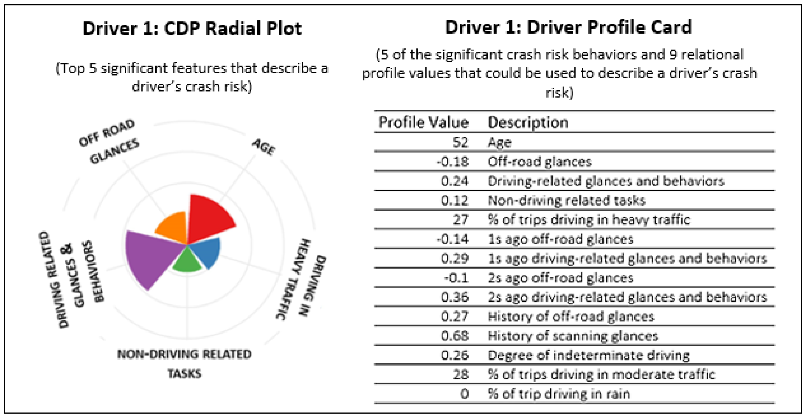
For each driver in the NEST dataset, their feature-complete variables () were used to develop and visualize their driver profiles through driver profile cards. Driver profile cards represent the minimum information required to associate a driver with their characteristics and behaviors that best explains their risk of crashing. Using driver profile cards, comparisons can be made by calculating relational CDP Scores for each driving behavior, determined by the standard deviations above and below the mean relative to the rest of the driving sample (Figure 5). The driver profiles can then be ranked by any of the features in the driver’s profile card or ranked in terms of the driver’s average risk as provided by the model.

Figure 5.
Example of a driver profile card using a radial plot and a profile value table to represent the 14 features (including the feature-complete set that was significantly associated with a driver’s risk of crashing). The radial plot shows 5 features (from the feature-complete set that best represented their risk of crashing), and the profile card had 9 additional variables representing their driving history behavior in general.
3.2. Comprehensive Driver Profile (CDP) Clusters
Drivers can also be clustered into profile groups as a means of exploring whether drivers can be grouped together into driver types based on their similarity to one another in their vehicle- and technology-usage patterns (as well as on their glance and task activity patterns). If so, a clustering of driver profiles may yield a typology of drivers. A driver typology could aid in developing strategies for customizing real-time driver support around common and uncommon types of drivers.
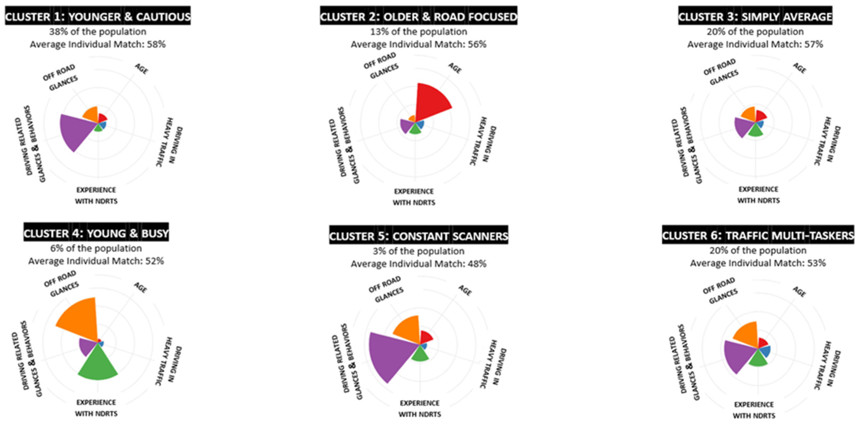
k-means clustering [34] was used to determine the range of the number of unique crash risk profile clusters among the NEST drivers. Cluster analyses revealed a total of six risky driver profile groups based on the top 14 significant feature contributors to crash risk. The six risky profile cluster types represented young and cautious drivers (38%, cluster 1), older and road focused (13%, cluster 2), simply average drivers (30%, cluster 3), young and busy (6%, cluster 4), constant scanners (3%, cluster 5), and traffic multi-taskers (20%, cluster 6) shown in Figure 6. The cluster names served as descriptors for understanding the key attributes that characterized the different types of risky driver groups. Based on these clusters, crash risk trends and individual commonalities can be uncovered. For example, cluster analysis showed that drivers in clusters 5 and 6 had traffic and driving situation that dominated these risk groups suggesting that these drivers had their crash risk influenced primarily by situational factors compared to drivers in the other clusters where their inherent driving behaviors most likely increased their risk of crashing.
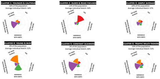
Figure 6.
Clustering NEST drivers based on their crash risk driver profiles.
3.3. Driver Profile Stability
In addition to assessing driver profile clusters, the driver’s goodness of matching with each cluster or driver profile ’type’ can also be determined. The underlying premise for this lies in both data and theory: Drivers do not always behave typically and, depending on the day, their behaviors, circumstances, and more driving- and non-driving-related variables may deviate from their typical or baseline style of driving or lifestyle [35]. Because of these differences, the CDPs and related CDP Scores can be used to understand how well a driver matches with any one cluster group. A driver’s goodness of matching to a cluster was determined by bootstrapping [36] and clustering of each driver to the original observed profile centers—each time recording which cluster/s the driver belongs to. Since bootstrapping allows simulation of a variety of trips the drivers take, it gives a notion of how often the driver moves from one cluster type to the other—representing their profile stability. Results of the bootstrapping are shown in Table 9 for a sample of 15 NEST drivers after conducting 100 bootstrap samples. In Table 9, the winning cluster column (Win Cluster) refers to the clusters the drivers most commonly belonged to, and the winning cluster percentage column (Win %) represents how often they landed in a cluster.
Table 9.
Bootstrapping example for 15 (out of 204) NEST drivers.
Results from the bootstrapping show that there are certain drivers that have high crash risk profile stability. For example, driver 15 in Cluster 2 (Table 9) had a 100% match to their profile cluster. These results indicate that even with limited data driver 15 might have a consistent crash risk profile associated with their older age and limited glances away from the road—suggesting that they do not conduct enough scanning glances to assess their driving environment. Whereas others that have lower crash risk profile stability, such as driver 1 in cluster 1 who had only a 38% match to their profile cluster. This result suggests that more data might be needed to better understand why their crash risk profile is not consistent and causes them to jump clusters. Thus, if this type of information could be fed into vehicle driver support and monitoring systems, it could help such systems more effectively adapt and tailor its warnings and cues to the individual, instead of adhering only to triggers and thresholds based on average behavior patterns across all drivers.
4. Discussion
The Comprehensive Driver Profile (CDP) framework proposed in this paper was used to develop driver profiles related to a driver’s risk of crashing and has many advantages that make it uniquely robust, flexible, and generalizable for different datasets. First, the approach used in the CDP framework outlines an approach to use all the driving behaviors and driving context as well as driver demographics to calculate a composite measure of risk—the CDP risk scores. The flexibility of the framework also enables the CDP scores to be calculated at different levels of granularity ranging from the driver level, trip level, epoch level, behavior level, to the moment-to-moment level for any outcome of interest. Thus, the framework enables profiles to be developed at the population level (which most driver profiles studies implement); but can also be adapted to the individual driver as well to account for and extract the relevant individual differences. Only one other study has implemented a driver profile framework that is adaptive to the individual driver, but the framework only focuses on pedal control behavior in its profiles [37].
Secondly, the CDP framework provides a detailed approach for including the associated interaction effects to build the driver profiles. This is important to highlight as a review of the current literature on driver profiles suggests limited work in the area of accounting for interaction effects within the driver profile and behavior frameworks, despite these studies showing that interaction effects, especially due to the driving environment and situation have a significant impact on the driving behavior [2,38].
Thirdly, there are a number of ‘driver type’ identification problems, wherein the research in this area has revealed fewer than 10 distinct classes of drivers due to the difficulty of developing discriminative group feature definitions [39,40]. The CDP framework provides a detailed approach on how to use the driver profiles and CDP scores for extracting insights and visualizations of driver types and individual differences. When dealing with a large population of drivers, generating not hundreds but thousands of driver profiles require there to be a methodology in place to make meaningful comparisons both at the population and individual level, which the CDP framework provides.
While this paper presents an improvement on current methods of building reliable and complete driver profiles, there are steps recommended in the framework that merit discussion—with opportunities for further improvement. For example, in the framework, dimension reduction using PCA is a necessary step for the effective analysis, visualization, and pre-processing of any driving dataset for building CDPs. However, for any high-dimensional naturalistic driving data, it is highly likely that the principle components (PC) from PCA will only have medium to low variance. This is because data sparseness for some of the glances and behaviors will result in a sparse matrix that increases the likelihood of requiring multiple PCs to maintain a majority of the variance. Additionally, the physiological nature of glances where more than one glance cannot occur at a time means that driving data at the sample level will always have inherent negative correlations resulting in PCA having weaker components.
In the CDP framework, a unique aspect of the Feature Selection stage is that the Random Forest is not used to create driver profiles, but instead used to identify which features may be removed, and which may be retained. However, an argument can be made that the Random Forest model should be used to create driver profiles because the model is likely to have very good accuracy, and potentially be better than the final model setup for constructing the driver profiles [41]. Although this was considered and is recommended in other driver profile frameworks, it is important to note that if the Random Forest model is implemented at the Feature Selection stage to develop driver profiles, a major drawback is that the list of features will be very long, and interpretation of the profiles is likely to be very difficult. Clustering driver profiles will also suffer drawbacks because a longer list of variables will result in sparse data that are difficult to segment. Future work will involve an in-depth analysis on the application of the CDP framework on larger datasets; assessing the robustness and generalizability of the CDP framework; and comparing the CDP framework against other established driver profile frameworks for real-time application and prediction. Despite its limitations at this early stage of development, and the many opportunities for its further development, the implementation of the CDP framework in its current form already holds a number of interesting and useful implications—and offers application possibilities that are highlighted below.
Implications for government and policy: There have been a number of government strategies aimed at improving road safety. Driver education and safety programs, along with traffic safety enforcement, strict penalties, changes to legislation, advertising campaigns, and graduated licensing schemes have been used to influence driving behaviors [42,43]. However, studies have found a weak relationship between the broad communication of risk and improvements in driving behavior, requiring the design of more targeted strategies to change how drivers perceive risk [44]. In this regard, comprehensive driver profiles can be used to assess the effectiveness of changes to infrastructure and legislation on road safety outcomes, both at the population level as well as the individual level, which could then be used to better understand the societal impacts of policy changes, and develop more effective road safety measures. Additionally, the ability to assess the full range of a driver’s profile (CDPs) within the specific spatial and temporal context of driving provides a unique opportunity to use these temporal and spatial factors for establishing ‘hard’ traffic calming measures [45] such as speed bumps—especially within specific areas of policy interest such as school zones, urban areas, and night time driving.
Implications for automotive manufacturers and automation: Despite significant efforts by government and road safety organizations to reduce risky driving, global statistics on road crashes, accidents, and injuries have shown that drivers continue to engage in risky driving behavior [46]. To improve road safety, driver support systems have much to offer by providing targeted feedback in real-time to reduce risky driving behavior [47]. However, the greatest difficulty in improving driver support system technologies is the lack of understanding regarding how to harness knowledge about different forms and patterns of safe and risky driving behaviors—along with a driver’s demographics, psychological profiles, risk perceptions, driving history, etc., to adequately target and customize feedback and support for that driver [48]. The CDP framework has enormous potential for contributing to the tailoring of driver support in real-time because it takes into consideration a particular driver’s needs in particular contexts.
The use of such comprehensive driver profiles are also becoming more relevant in the field of automation as companies move toward driver-out-of-the-loop automation system capabilities [49]. The ability to understand the driver provides opportunities for driverless cars to drive like humans, thereby improving the trust, adherence, and comfort that humans have with the automation [50]. Additionally, as the field of automation moves into the human-machine collaborative space, comprehensive driver profiles can not only be used for a wide variety of applications to support the driver and their collaborative role with the automation, but also by helping the automation determine the role of the driver during different situations, such as when to accede and secede driving control based on the driver’s ability.
Implications for insurance telematics: Insurance companies use varying amounts of driver profile scoring models, mainly focused on variables such as acceleration and braking, and the degree to which they are rapid or harsh—as well as absolute and relative speeding, swerving, and cornering; along with trip-related factors such as trip duration, distance, time of day, and location as the best predictors of risk [51,52,53]. While developing profile scores using these types of measures has been useful in determining the differences between demographic groups that are over- and under-represented in crashes, the domain has two important challenges. First, many current driver risk profiles are based on population models and ignore the heterogeneity of driving behaviors among individual drivers [1], which is important for usage-based-insurance (UBI) and pay-as-you-drive (PAYD) plans. Second, the high dimensionality of naturalistic driving data and inherent heterogeneity of driving behaviors requires establishing methodologies to ensure robustness and flexibility in generating reliable driver risk profiles that correlate with the actual risk of the driver [54]. Preliminary results from implementing the CDP framework suggest that it would be useful for addressing these challenges—especially for assessing individual differences. The CDP framework could be used to gain more accurate insights on what programs work best for certain types of drivers or individuals, providing financial incentives for improving risky driving behaviors, and rewarding drivers with good driving scores. Using CDP should also lead to more accurate pricing for usage-based insurance, given the broader set of variables upon which it is based.
In spite of many improvements in safety technology over the last several decades, automotive crashes continue to claim thousands of lives per year, for example, an average of 36,475 fatalities per year between 2005 and 2018 [55]. Additionally, NHTSA has reported that driver-related critical factors may account for 92% to 96% of crashes [56] based on data from the US National Motor Vehicle Crash Causation Survey (NMVCCS). Thus, the substantial role played by human behaviors and errors in crashes has been well established for many years. Yet models of crash risk have struggled to account for a preponderance of the variance in the data. Indeed, even efforts to account for crash risk in more-specifically focused areas such as distraction-related crash risk have foundered because of wide differences between behaviors of individual drivers—and an inability of models to account for, explain, or harness individualized patterns of behavior in accounting for driving styles and risk-related outcomes. An early naturalistic study showed that a small percentage of drivers accounted for a very large proportion of the observed safety-critical events—and noted that the driving behaviors of this small segment of drivers were different from other drivers, insofar as they were characterized by more hard decelerations, hard accelerations and swerve maneuvers [57]. When the full sample of drivers was divided into three groups by [57] into unsafe, moderately safe, and safe drivers based on number of crashes-and-near-crashes observed for each, the 15 drivers placed in the unsafe group made 2112.8 safety-critical-events per million vehicle miles traveled (MVMT) during the 100-Car study (vs. 460.0 events per MVMT for the moderately safe group of 47 drivers, and 63.1 events per MVMT observed for the safe group of 39 drivers). Yet, in spite of wide and acknowledged differences of this sort between drivers, it has often been the case that in analyses of risk ratios—as well as in approaches to modeling risk—differences between drivers have either been ignored (and all safety-critical events pooled in analyses)—or driver differences have often tended to be treated as “noise” or “error” variance that obscures the “true” effects of important underlying variables (which are believed to be, for example, driving experience variables, vehicle design variables, roadway context, or weather variables).
However, the work described herein takes a different approach. Drawing from research traditions in adjoining fields—the notion explored here is that the very essence of understanding crash risk lies in the variance between individuals. In other words, it is this variance between individual drivers in their driving behavior and driving style that embodies the very information about crash risk from which meaning and understanding must be drawn. This variance is not “noise” or “error”—to be apportioned into a statistical error term for a group of drivers, nor for an individual driver. Rather, it is the central object of study. It is by applying techniques that have the power to extract “behavioral patterns over time,” along with techniques for identifying or selecting those that are most important in accounting for specific outcomes (such as crashes vs. successful crash-free driving)—and techniques which enable these “patterns” to be treated as “features” that can be attributed to different types of drivers—that there is a chance to advance and deepen the scientific understanding of crash risk (or other outcomes), and begin to account for it. There may even be an opportunity, using these methods, to predict crash risk for individual drivers—or for groups of drivers. This paper therefore suggests an initial framework for use in exploring whether a deeper understanding of risk in driving can be extracted from this variance—the differences between individual drivers—and systematically understanding its underlying structure.
5. Conclusions
Driving is a complex task, and drivers are constantly confronted with situations in which they must make a decision about their reaction to the environment or driving situation or both. Those daily situations such as changing lanes to make an exit are reflections of a driver’s inherent driving style and behavior. Additionally, the ability to record these behaviors over time, and to extract the information and patterns within them, provides the foundation upon which driver support systems can be tailored to better support the driver and provide targeted safety benefits, but an important challenge when dealing with such vast and granular temporospatial driving behavior data is the proper analyses and interpretation of the data to understand the driver’s choice, preferences, comfort, trust in technology, risk aversion, etc., which, when successfully extracted, would allow for more meaningful tailoring of the driver support system to the individual.
To address this challenge, this paper has proposed a practical, novel, data-driven framework for developing comprehensive driver profiles. The framework is composed of three steps which allows for cleaning, enriching, profiling, scoring, visualization, analyses, and interpretation of a wide range of driving behaviors, context, and interaction effects, which can be used to calculate any outcome of interest (risk, inattention, fatigue, etc.). The main advantage of such a framework is its adaptive approach that considers the environmental and situational conditions and continuously updates the driver’s profile based on these inputs. This has important implications for personalizing real-time feedback, support, and safety measures that is adaptable to the individual driver.
Author Contributions
Conceptualization, R.P.P. and L.S.A.; methodology, primarily R.P.P., some ideas from L.S.A.; formal analysis, R.P.P. and L.S.A. with review by L.S.A.; writing—original draft preparation, primarily R.P.P.; some input from L.S.A.; writing—review and editing, primarily R.P.P. and some input from L.S.A.; and visualization, R.P.P. and L.S.A. All authors have read and agreed to the published version of the manuscript.
Funding
This research was funded by the Advanced Vehicle Technology (AVT) Consortium and the Advanced Human Factors Evaluator for Automotive Demand (AHEAD) Consortium, led by MIT.
Institutional Review Board Statement
The MIT Committee On the Use of Humans as Experimental Subjects (COUHES) reviewed IRB submission (Protocol # 1603520858) which requested permission to use the SHPR2 NEST database for secondary analyses under the terms of a Data Usage License (see under Informed Consent Statement) granted by Virginia Tech Transportation Institute, the licensing agent for this database. The COUHES decision (after review) was that this research was exempt (dated 8 April 2016).
Informed Consent Statement
Informed consent was obtained from the participants in the original SHRP2 study from which the NEST dataset was drawn. The analyses done here are secondary analyses performed on data that had already been collected previously—and, thus, there was no direct contact with participants—all of whom had given consent at the time of data collection at a prior date. If needed, further information about the SHRP2 study, the terms of the original IRB review, original Informed Consent, and the original ethics oversight for the SHRP2 study (which was overseen by the Transportation Research Board of the National Academies) can be obtained here at the Federal Highway Administration website: https://www.fhwa.dot.gov/goshrp2/About, accessed on 8 April 2016. As part of the original Informed Consent Statement and procedures of the original SHRP2 study, participants consented to the subsequent use of their data for secondary analysis by other research entities if done under the provisions of a Data Usage License (DUL) administered by VTTI. Such a Data Usage License for the use of the NEST dataset (which was itself a derivative of the SHRP2 data) was obtained by MIT from VTTI to support the research.
Data Availability Statement
The Naturalistic Engagement in Secondary Tasks (NEST) data set is the product of a prior collaboration between the Virginia Tech Transportation Institute (VTTI) and the Toyota Collaborative Safety Research Center (Toyota CSRC). The purpose of the project was to develop a dataset that would enable users to study multiple aspects of secondary task involvement including factors which may contribute to distraction and to distraction-related safety-critical events (SCEs) that include a crash or near-crash (C/NC). The dataset also includes baseline epochs. The dataset is available to researchers, providing de-identified, highly detailed time-series data as well as additional high-level data about both secondary task engagement and distraction-related SCEs during real-world driving. Further information about this data and information regarding specific variables in the data set can be found in the accompanying NEST Data Dictionary available through VTTI https://doi.org/10.15787/VTT1/OZQ6BL (accessed on 8 January 2019).
Acknowledgments
Support for the work was provided by the Advanced Vehicle Technology (AVT) Consortium and the Advanced Human Factors Evaluator for Automotive Demand (AHEAD) Consortium at MIT. The views and conclusions expressed are solely those of the authors and have not been sponsored, approved, or endorsed by either Consortium. The authors thank colleagues at Touchstone, the MIT AgeLab, and the Consortia for their reviews of earlier drafts.
Conflicts of Interest
The authors declare no conflict of interest. This program of research was free from any biasing or controlling interests of a financial, commercial, political, personal, or adversarial nature.
References
- De Winter, J.C.F.; Happee, R. Modelling Driver Behaviour: A Rationale for Multivariate Statistics. Theor. Issues Ergon. Sci. 2012, 3, 528–545. [Google Scholar] [CrossRef]
- Abdelrahman, A. Driver Behavior Modelling and Risk Profiling Using Large-Scale Naturalistic Driving Data. Ph.D. Thesis, Queen’s University, Kingston, ON, Canada, 2019. [Google Scholar]
- Sagberg, F.; Selpi; Piccinini, G.F.B.; Engström, J. A Review of Research on Driving Styles and Road Safety. Hum. Factors J. Hum. Factors Ergon. Soc. 2015, 57, 1248–1275. [Google Scholar] [CrossRef] [PubMed]
- Griesche, S.; Krähling, M.; Käthner, D. Conform—A Visualization Tool and Method to Classify Driving Styles in Context of Highly Automated Driving. VDI/VW Gem. Fahr. Integr. Sich. 2014, 30, 101–110. [Google Scholar]
- Toledo, T.; Musicant, O.; Lotan, T. In-vehicle data recorders for monitoring and feedback on drivers’ behavior. Transp. Res. Part C Emerg. Technol. 2008, 16, 320–331. [Google Scholar] [CrossRef]
- Jun, J. Potential Crash Measures Based On Gps-Observed Driving Behavior Activity Metrics. Ph.D. Thesis, Georgia Institute of Technology, Atlanta, GA, USA, 2006. [Google Scholar]
- Bagdadi, O.; Várhelyi, A. Jerky Driving—An Indicator of Accident Proneness? Accid. Anal. Prev. 2011, 43, 1359–1363. [Google Scholar] [CrossRef]
- Ellison, A.B.; Greaves, S.P.; Bliemer, M.C. Driver behaviour profiles for road safety analysis. Accid. Anal. Prev. 2015, 76, 118–132. [Google Scholar] [CrossRef]
- Shope, J.T. Influences on youthful driving behavior and their potential for guiding interventions to reduce crashes. Inj. Prev. 2006, 12, i9–i14. [Google Scholar] [CrossRef]
- Ellickson, P.L.; Tucker, J.S.; Klein, D.J.; Saner, H. Antecedents and Outcomes of Marijuana Use Initiation during Adolescence. Prev. Med. 2004, 39, 976–984. [Google Scholar] [CrossRef]
- Bina, M.; Graziano, F.; Bonino, S. Risky driving and lifestyles in adolescence. Accid. Anal. Prev. 2005, 38, 472–481. [Google Scholar] [CrossRef]
- Strayer, D.L.; Drews, F.A. Profiles in Driver Distraction: Effects of Cell Phone Conversations on Younger and Older Drivers. Hum. Factors J. Hum. Factors Ergon. Soc. 2004, 46, 640–649. [Google Scholar] [CrossRef]
- Júnior, J.F.; Carvalho, E.; Ferreira, B.V.; de Souza, C.; Suhara, Y.; Pentland, A.; Pessin, G. Driver Behavior Profiling: An Investigation with Different Smartphone Sensors and Machine Learning. PLoS ONE 2017, 12, e0174959. [Google Scholar]
- Chang, W. Research on Driving Intention Identification Based on Hidden Markov Model. Master’s Thesis, Jilin University, Changchun, China, 2011. [Google Scholar]
- Mei, N.N.; Wang, Z.J. Moving Object Detection Algorithm Based on Gaussian Mixture Model. Comput. Eng. Des. 2012, 33, 3149–3153. [Google Scholar]
- Tramèr, F.; Zhang, F.; Juels, A.; Reiter, M.K.; Ristenpart, T. Stealing Machine Learning Models via Prediction Apis. arXiv 2016, arXiv:1609.02943. [Google Scholar]
- Castignani, G.; Derrmann, T.; Frank, R.; Engel, T. Driver Behavior Profiling Using Smartphones: A Low-Cost Platform for Driver Monitoring. IEEE Intell. Transp. Syst. Mag. 2015, 7, 91–102. [Google Scholar] [CrossRef]
- Owens, J.M.; Angell, L.; Hankey, J.M.; Foley, J.; Ebe, K. Creation of the Naturalistic Engagement in Secondary Tasks (NEST) distracted driving dataset. J. Saf. Res. 2015, 54, 33.e29–36. [Google Scholar] [CrossRef] [Green Version]
- Antin, J.; Lee, S.; Hankey, J.; Dingus, T. Design of the In-Vehicle Driving Behavior and Crash Risk Study. In Support of the SHRP 2 Naturalistic Driving Study; Strategic Highway Research Program Safety Focus Area; Transportation Research Board: Washington, DC, USA, 2011. [Google Scholar]
- Dingus, T.A.; Guo, F.; Lee, S.; Antin, J.F.; Perez, M.; Buchanan-King, M.; Hankey, J. Replication Data for: Driver crash risk factors and prevalence evaluation using naturalistic driving data. Proc. Natl. Acad. Sci. USA 2016, 113, 2636–2641. [Google Scholar] [CrossRef] [Green Version]
- Lewis, E.; Sheridan, C.; O’Farrell, M.; King, D.; Flanagan, C.; Lyons, W.; Fitzpatrick, C. Principal component analysis and artificial neural network based approach to analysing optical fibre sensors signals. Sens. Actuators A Phys. 2007, 136, 28–38. [Google Scholar] [CrossRef]
- Bommert, A.; Sun, X.; Bischl, B.; Rahnenführer, J.; Lang, M. Benchmark for filter methods for feature selection in high-dimensional classification data. Comput. Stat. Data Anal. 2019, 143, 106839. [Google Scholar] [CrossRef]
- Hand, D.J.; Till, R.J. A Simple Generalisation of the Area Under the Roc Curve for Multiple Class Classification Problems. Mach. Learn. 2001, 45, 171–186. [Google Scholar] [CrossRef]
- Anukrishna, P.R.; Paul, V. A Review on Feature Selection for High Dimensional Data. In Proceedings of the 2017 International Conference on Inventive Systems and Control (ICISC), Coimbatore, India, 19–20 January 2017; pp. 1–4. [Google Scholar]
- Chen, T.; Guestrin, C. Xgboost: A Scalable Tree Boosting System. In Proceedings of the 22nd ACM Sigkdd International Conference On Knowledge Discovery and Data Mining, San Francisco, CA, USA, 13–17 August 2016; pp. 785–794. [Google Scholar]
- Liaw, A.; Wiener, M. Classification and Regression By Randomforest. R News 2002, 2, 18–22. [Google Scholar]
- Breiman, L. Random Forests. Mach. Learn. 2001, 45, 5–32. [Google Scholar] [CrossRef] [Green Version]
- Breiman, L.; Cutler, A. Random Forest. 1995. Available online: https://www.Stat.Berkeley.Edu/~Breiman/Randomforests/ (accessed on 6 February 2021).
- Xu, R.; Nettleton, D.; Nordman, D.J. Case-Specific Random Forests. J. Comput. Graph. Stat. 2016, 25, 49–65. [Google Scholar] [CrossRef]
- Hastie, T.J. Generalized Additive Models; Routledge: Boca Raton, FL, USA, 2017. [Google Scholar]
- Derksen, S.; Keselman, H.J. Backward, forward and stepwise automated subset selection algorithms: Frequency of obtaining authentic and noise variables. Br. J. Math. Stat. Psychol. 1992, 45, 265–282. [Google Scholar] [CrossRef]
- Pan, W. Akaike’s Information Criterion in Generalized Estimating Equations. Biometrics 2001, 57, 120–125. [Google Scholar] [CrossRef]
- Weisstein, E.W. Bonferroni Correction. 2004. Available online: https://mathworld.wolfram.com/ (accessed on 23 May 2021).
- Charrad, M.; Ghazzali, N.; Boiteau, V.; Niknafs, A. Nbclust: An R Package for Determining the Relevant Number of Clusters In A Data Set. Ournal of Statistical Software 2014. Available online: Http://Www.Jstatsoft.Org/V61/I06/ (accessed on 4 March 2021).
- Lewis-Evans, B.; de Waard, D.; Brookhuis, K.A. Speed maintenance under cognitive load—Implications for theories of driver behaviour. Accid. Anal. Prev. 2011, 43, 1497–1507. [Google Scholar] [CrossRef] [Green Version]
- Abney, S. Bootstrapping. In Proceedings of the 40th Annual Meeting of the Association for Computational Linguistics, Philadephia, PA, USA, 6–12 July 2002; Association for Computational Linguistics: Philadelphia, PA, USA, 2002; pp. 360–367. [Google Scholar]
- Angkititrakul, P.; Ryuta, T.; Wakita, T.; Takeda, K.; Miyajima, C.; Suzuki, T. Evaluation Of Driver-Behavior Models In Real-World Car-Following Task. In Proceedings of the 2009 IEEE International Conference on Vehicular Electronics and Safety (ICVES), Pune, India, 11–12 November 2009; pp. 113–118. [Google Scholar]
- Ericsson, E. Variability in urban driving patterns. Transp. Res. Part D Transp. Environ. 2000, 5, 337–354. [Google Scholar] [CrossRef]
- Dong, W.; Li, J.; Yao, R.; Li, C.; Yuan, T.; Wang, L. Characterizing Driving Styles with Deep Learning. arXiv 2016, arXiv:1607.03611. [Google Scholar]
- Lin, N.; Zong, C.; Tomizuka, M.; Song, P.; Zhang, Z.; Li, G. An Overview on Study of Identification of Driver Behavior Characteristics for Automotive Control. Math. Probl. Eng. 2014, 2014, 569109. [Google Scholar] [CrossRef]
- Petkovic, D.; Altman, R.B.; Wong, M.; Vigil, A. Improving The Explainability of Random Forest Classifier-User Centered Approach. Pac. Symp. Biocomput. 2018, 23, 204–215. [Google Scholar]
- Watsford, R. The Success of the ’pinkie’ Campaign-Speeding. No One Thinks Big of You: A New Approach to Road Safety Marketing. In Proceedings of the Australasian College of Road Safety Conference, Washington, DC, USA, 9–13 January 2008; pp. 390–395. [Google Scholar]
- Faulks, I. Road Safety Advertising And Social Marketing. J. Australas. Coll. Road Saf. 2011, 22, 27. [Google Scholar]
- Lund, J.; Aarø, L. Accident prevention. Presentation of a model placing emphasis on human, structural and cultural factors. Saf. Sci. 2004, 42, 271–324. [Google Scholar] [CrossRef]
- Edquist, J.; Rudin-Brown, C.M.; Lenné, M.G. The Effects of On-Street Parking and Road Environment Visual Complexity on Travel Speed and Reaction Time. Accid. Anal. Prev. 2012, 45, 759–765. [Google Scholar] [CrossRef]
- World Health Organization. Global Status Report on Road Safety; World Health Organization: Geneva, Switzerland, 2015. [Google Scholar]
- Richter, M.; Pape, H.C.; Otte, D.; Krettek, C. Improvements In Passive Car Safety Led To Decreased Injury Severity–A Comparison Between the 1970s and 1990s. Injury 2005, 36, 484–488. [Google Scholar] [CrossRef] [PubMed]
- Ellison, A.B. Evaluating Changes in Driver Behaviour for Road Safety Outcomes: A Risk Profiling Approach. Ph.D. Thesis, The University of Sydney, Sydney, Australia, 2013. [Google Scholar]
- SAE. Surface Vehicle Recommended Practice; SAE: Warrendale, PA, USA, 2016. [Google Scholar]
- Lee, J.D.; See, K.A. Trust in Automation: Designing for Appropriate Reliance. Hum. Factors 2004, 46, 50–80. [Google Scholar] [CrossRef] [PubMed]
- Pyta, V.; Mctiernan, D. Development of A Model for Improving Safety in School Zones. In Proceedings of the Australasian Road Safety Research, Policing and Education Conference, Monash University, Melbourne, Australia, 31 August–3 September 2010. [Google Scholar]
- Litman, T. Distance-Based Vehicle Insurance Feasibility, Costs and Benefits; Victoria Transport Policy Institute: Victoria, BC, Canada, 2007. [Google Scholar]
- Ong, P.M.; Stoll, M.A. Why Do Inner City Residents Pay Higher Premiums? The Determinants of Automobile Insurance Premiums; School of Public Affairs: Los Angeles, CA, USA, 2008. [Google Scholar]
- Handel, P.; Skog, I.; Wahlstrom, J.; Bonawiede, F.; Welch, R.; Ohlsson, J.; Ohlsson, M. Insurance Telematics: Opportunities and Challenges with the Smartphone Solution. IEEE Intell. Transp. Syst. Mag. 2014, 6, 57–70. [Google Scholar] [CrossRef]
- Regan, M.A.; Prabhakharan, P.; Wallace, P.; Cunningham, M.L.; Bennett, J.M. Education and Training for Drivers of Assisted and Automated Vehicles; ARRB Group Limited: Sydney, Australia, 2020. [Google Scholar]
- NHTSA. Federal Automated Vehicles Policy–Accelerating the Next Revolution in Roadway Safety; NHTSA: Washington, DC, USA, 2016.
- Klauer, S.G.; Dingus, T.A.; Neale, V.L.; Sudweeks, J.D.; Ramsey, D.J. Comparing Real-World Behaviors of Drivers With High versus Low Rates of Crashes and Near-Crashes; NHTSA: Washington, DC, USA, 2009.
Publisher’s Note: MDPI stays neutral with regard to jurisdictional claims in published maps and institutional affiliations. |
© 2022 by the authors. Licensee MDPI, Basel, Switzerland. This article is an open access article distributed under the terms and conditions of the Creative Commons Attribution (CC BY) license (https://creativecommons.org/licenses/by/4.0/).