
GenericConv: A Generic Model for Image Scene Classification Using Few-Shot Learning


1
Bioinformatics Program, Faculty of Computer and Information Sciences, Ain Shams University, Cairo 11566, Egypt
2
Information Systems Department, Faculty of Computer and Information Sciences, Ain Shams University, Cairo 11566, Egypt
*
Author to whom correspondence should be addressed.
Information 2022, 13(7), 315; https://doi.org/10.3390/info13070315
Submission received: 5 April 2022
/
Revised: 8 May 2022
/
Accepted: 13 May 2022
/
Published: 28 June 2022
(This article belongs to the Topic Big Data and Artificial Intelligence)
Abstract
:Scene classification is one of the most complex tasks in computer-vision. The accuracy of scene classification is dependent on other subtasks such as object detection and object classification. Accurate results may be accomplished by employing object detection in scene classification since prior information about objects in the image will lead to an easier interpretation of the image content. Machine and transfer learning are widely employed in scene classification achieving optimal performance. Despite the promising performance of existing models in scene classification, there are still major issues. First, the training phase for the models necessitates a large amount of data, which is a difficult and time-consuming task. Furthermore, most models are reliant on data previously seen in the training set, resulting in ineffective models that can only identify samples that are similar to the training set. As a result, few-shot learning has been introduced. Although few attempts have been reported applying few-shot learning to scene classification, they resulted in perfect accuracy. Motivated by these findings, in this paper we implement a novel few-shot learning model—GenericConv—for scene classification that has been evaluated using benchmarked datasets: MiniSun, MiniPlaces, and MIT-Indoor 67 datasets. The experimental results show that the proposed model GenericConv outperforms the other benchmark models on the three datasets, achieving accuracies of 52.16 ± 0.015, 35.86 ± 0.014, and 37.26 ± 0.014 for five-shots on MiniSun, MiniPlaces, and MIT-Indoor 67 datasets, respectively.
1. Introduction
Scene classification (SC) is a complex task that relies on other sub-tasks, including object detection (OD), object classification (OC), and texture classification. By employing object detection in the scene classification, accurate results could be achieved as prior knowledge about objects that exist in the scene will lead to an easier interpretation of the image content. In contrast, semantic areas and knowledge about objects present in the image may infer the scene type more precisely [1,2].
Machine learning is widely used in scene classification in both tasks: object detection and object classification. Even though machine learning and deep learning achieved optimal performance in simple tasks, such as object detection, which led to their usage in more complex tasks, such as image scene classification, there is still a wide area of improvement that could be performed. The models’ training phases need a significant quantity of data, which is a challenging and time-consuming task. Furthermore, most models rely on data from the training set, which results in useless models that can only detect samples that are comparable to the training set. These limitations lead to the use of few-shot learning in computer-vision tasks. Given the optimal performance of few-shot learning in object detection, few attempts have been made in scene classification, including a few datasets for model evaluation. It is a fact that research in this area is still ongoing and rising by the day, but it still faces a number of obstacles.
In this work, we propose a few-shot learning model that tackles the scene classification challenge. By being generalized on three popular scene datasets, the model will overcome the constraints of previously described models in scene categorization research regarding the generalization of models and the classification accuracy.
Our proposed pipeline addresses the generalization of the scene classification task by implementing a novel model that achieved unprecedented performance compared to the previously reported models on three benchmarked datasets. Furthermore, the usability of a new dataset rather than the used datasets to confirm the generalizability and validity of our proposed model.
The rest of the paper is organized as follows. The following section gives a brief literature review that highlights the limitations of scene classification research work. Then, benchmark approaches, datasets, and evaluation metrics are presented. The proposed model is then discussed. Experimental results obtained are then described. Finally, the conclusion and direction for future work are presented.
2. Related Work
Scene classification is considered one of the most complex tasks in computer vision research as it involves two other subtasks: object detection and object classification. The interconnection between the aforementioned tasks makes it harder to achieve accurate results in scene classification. Researchers apply the logistic solution by solving the two subtasks with optimal performance, which will lead to accurate results in scene classification. Scene classification approaches are divided into two categories: machine/deep learning algorithms and few-shot learning algorithms. Machine learning and deep learning algorithms seek to optimize model accuracy on specific datasets, whereas few-shot learning techniques seek generalizability. The categories of scene classification approaches are presented in the following sub-sections.
2.1. Machine Learning Approaches
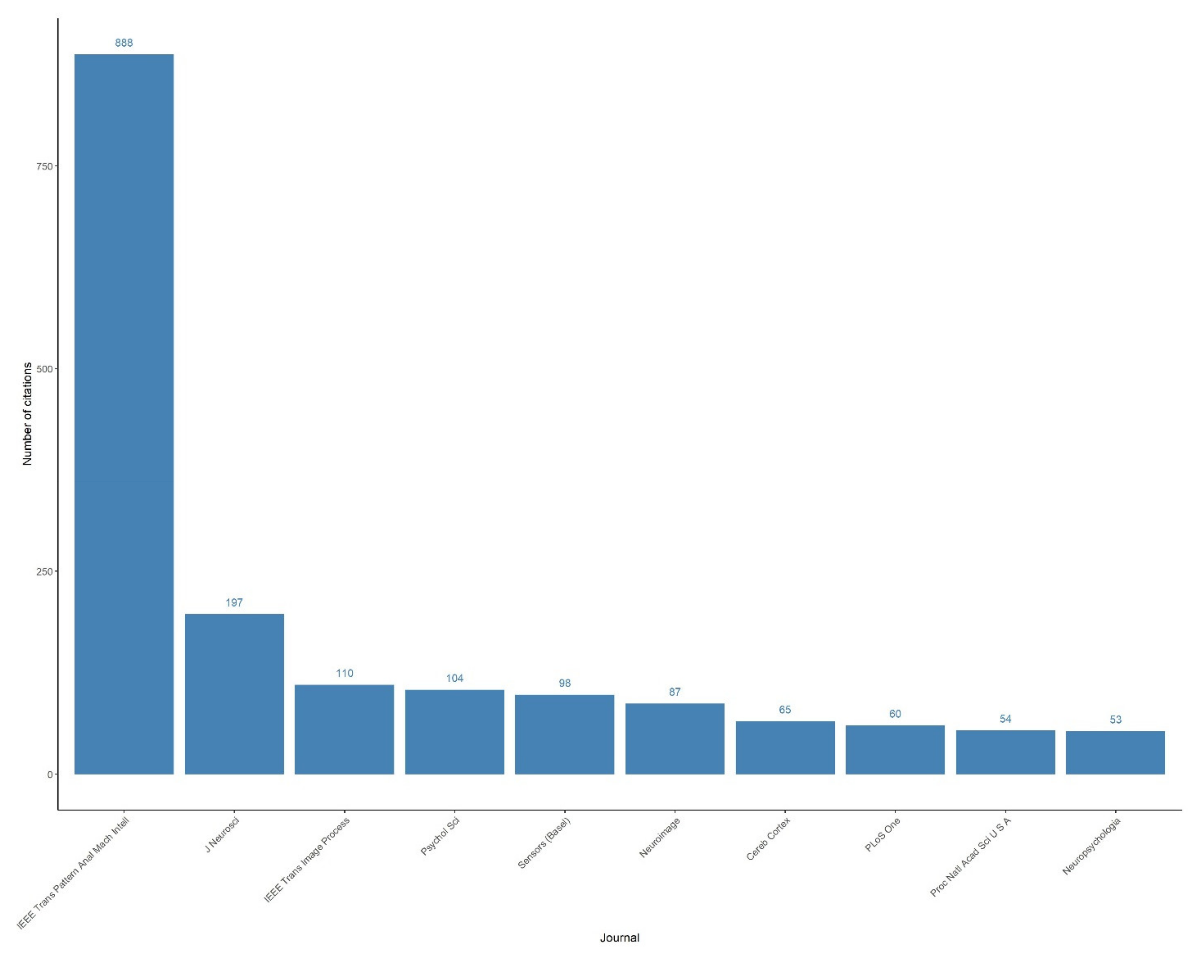
Many attempts have been made at object detection using machine learning and deep learning, as the goal of object detection is to create computational models and approaches that give one of the most fundamental bits of data required by computer vision applications. Furthermore, due to the adequateness of datasets and technologies in recent decades, machine learning, and deep learning have been employed in computer vision to extract knowledge and information from complex images [3]. Many attempts were made in the era of scene categorization using diverse methodologies, as shown in Figure 1.
The first subtask is object detection, in which algorithms can be classified into three main categories: traditional detectors, Conventional Neural Network (CNN)-based two-stage detectors, and CNN-based one-stage detectors [4]. Initially, classical detectors were inspired by P. Viola and M. Jones’ work 20 years ago, which designed a sliding window to iterate over picture pixels and recognize faces in any window.
Furthermore, to increase accuracy, a Histogram of Oriented Gradient (HOG) is utilized, which is computed on a dense grid of regularly spaced cells with overlapping local contrast normalization (on “blocks”) [5,6,7]. The deep learning approach relies on the architecture of Conventional Neural Networks (CNNs). It is an extension of the Neural Networks (NNs) but with modifications in the connections between layers to ignore less important features and include the vital features that will be used in the classification task. CNN is the most used algorithm in deep learning that extracts the vital features from the image using the Conventional layer that applies a filter to an image to produce a feature map that describes the detection of features in the input. Then, it passes the output features to the pooling layer that down-samples the feature map by sliding a two-dimensional filter over each channel of the feature map and summing the features inside the filter’s region. The last layer is the fully connected layer which is the feed-forward layer that compiles the final output as a probability assigned to each class of the input data representing the weights.
Moreover, as data and technology increased, CNN-based two-stage detectors were adopted due to their capacity to extract critical information from complicated pictures. Eventually, CNN-based one-stage detectors were utilized to achieve optimal accuracy in object recognition algorithms such as Single Shot multi-box Detector (SSD) and You Only Look Once (YOLO), which were extensively employed owing to their accurate time and accuracy performance [8,9].
The second subtask is object classification, in which researchers seek to educate the computer to mimic human brain functions by learning from past knowledge or experience. The learning process begins with feeding the model training data including labels for each image, and the model attempts to learn the pattern that maps the input images to their labels. Then, we use unseen test images to evaluate the learned model.
For image classification, various models were employed initiated by Alex Krizhevsky that was the primary designer of AlexNet. AlexNet rose to prominence after competing in the ImageNet Large Scale Visual Recognition Challenge [10,11]. It had a top-5 mistake rate of 15.3%. This was 10.8% less than the runner-up. The original paper’s main finding was that the depth of the model was definitely necessary for its excellent performance. This was highly computationally expensive, but it was made possible by GPUs, or Graphical Processing Units, during training. AlexNet has five convolutional layers, three max-pooling layers, two normalization layers, two fully connected layers, and one softmax layer. Convolutional filters and a nonlinear activation function ReLU are used in each convolutional layer. To maximize pooling, the pooling layers are utilized. The input size is mentioned at most of the places as 224 × 224 × 3 but due to some padding which happens it works out to be 227 × 227 × 3.
In 2013, ZFNet came out on top in the ImageNet Large Scale Visual Recognition Challenge (ILSVRC) with a substantial improvement over AlexNet. This work is a gold nugget that serves as a foundation for numerous concepts, including deep feature visualization, feature invariance, feature evolution, and feature significance. ZFNet is a modified version of AlexNet that provides more accuracy.
The techniques differed significantly in that ZF Net utilized 7 × 7 filters whereas AlexNet used 11 × 11 filters. The reasoning behind this is that they were losing a lot of pixel information by using larger filters, which can be kept by using lower filter sizes in the early conv layers. As they go deeper, the number of filters increases. This network, like others, uses ReLUs for activation and was trained using batch stochastic gradient descent [12]. In 2013, VGG was first proposed, and it finished second in the ImageNet competition in 2014. In comparison to AlexNet and ZFNet, it is commonly utilized as a basic design. VGG Net employed 3 × 3 filters, whereas AlexNet used 11 × 11 filters and ZFNet used 7 × 7 filters. The authors explain that having small repetitive fields of small filters as 3 × 3 filters offers an effective receptive field of 5 × 5, and 3–3 × 3 filters give a receptive field of 7 × 7 filters, but utilizing this we can train the network with a much less number of hyper-parameters [12].
In 2014, numerous excellent models were created, including VGG, however, GoogleNet emerged as the winner of the ImageNet competition. GoogleNet developed an inception module, which comprises skipping network connections to produce a tiny module, which is replicated throughout the network. GoogleNet employs nine inception modules and removes all fully connected layers by average pooling to reduce the size of the network from 7 × 7 × 1024 to 1 × 1 × 1024. This saves a large number of parameters [12].
The Microsoft ResNet protocol has 152 layers. The authors demonstrated empirically that when more layers are added, the error rate should decrease, in contrast to “simple nets,” by adding a few layers that lead to larger training and test mistakes. On an 8 GPU computer, it took two to three weeks to train. One apparent reason why residual blocks increase classification is the direct step from one layer to the next, and intuitively employing all of these skip steps builds a gradient highway where the gradients computed may directly alter the weights in the first layer, making updates have a greater effect [13]. ResNet-50, another version of ResNet is a convolutional neural network that is 50 layers deep and developed by some researchers from the Microsoft research group. The architecture is designed to overcome the theory of vanishing gradient phenomena in models, such as AlexNet and VGG. The input layers of this network are made up of many residual blocks, and the operating idea is to optimize a residual function. Furthermore, ResNet won first place in ILSVRC and COCO 2015 competitions [12,13].
The pre-trained version of the network is trained on more than a million images from the ImageNet dataset. The pre-trained network can classify images into 1000 object categories, such as keyboard, mouse, pencil, and many animals. As a result, the network has learned rich feature representations for a wide range of images. The network has an image input size of 224-by-224.
Other versions of ResNet architecture were proposed including ResNet-50 (Places architecture) which is the same architecture as ResNet-50 but is trained on the places dataset, ResNet-101 which is a convolutional neural network that is 101 layers deep, and Squeeze-and-Excitation (SE) ResNext 101 is a convolutional neural network that is 101 layers deep. The pre-trained version of the network is trained on more than a million images from the ImageNet dataset. Recently, various approaches and variants of the ResNet model were implemented and show a better performance than the original architecture [14,15,16]. The architectures are shown in Table 1 below.
2.2. Few-Shot Learning Approaches
Few-shot learning arises to solve the existing limitations of machine learning approaches. Despite the optimal performance of the existing machine and deep learning models in image understanding and scene classification, there are still major issues. First, the training phase for the models necessitates a large amount of data, which is a difficult and time-consuming task. Furthermore, most models are reliant on data previously seen in the training set, resulting in ineffective models that can only identify samples that are similar to the training set.
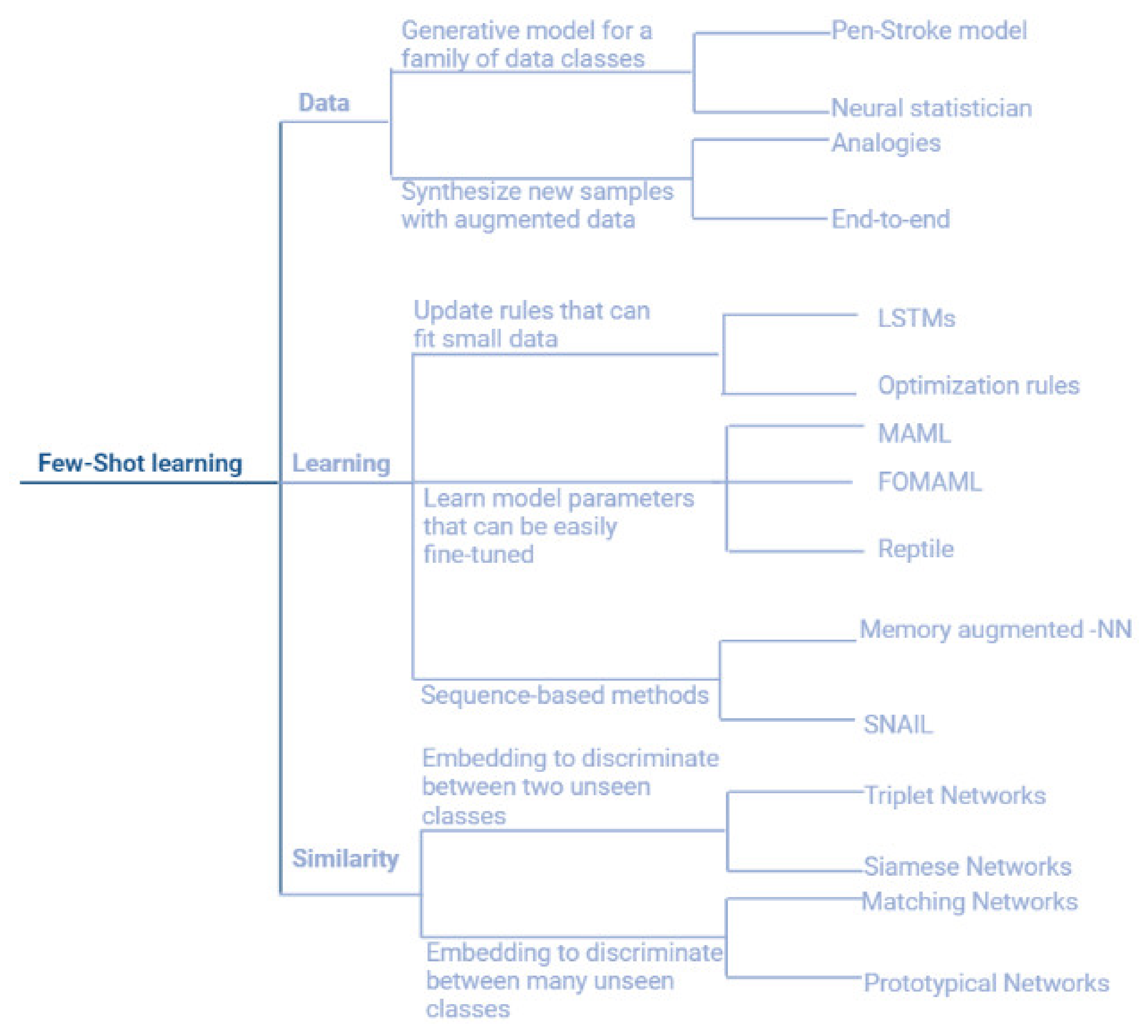
Few-shot learning can be categorized into three main approaches: data, similarity, and learning. The data approach exploits prior knowledge about the structure and the variability of the data, which enables the construction of viable models through a few samples. This category involves the Pen-Stroke models which are the smart interface that automatically extracts and refines pen strokes from images of hand-drawn sketches, and neural statistician, a variational autoencoder extension that can learn a method for computing unsupervised representations, or statistics, of datasets. For each dataset, the network is trained to create statistics that embody a generative model. As a result, the network is capable of learning from fresh datasets efficiently for both unsupervised and supervised tasks. Researchers demonstrate that networks can learn statistics for grouping datasets, transferring generative models to new datasets, picking representative dataset samples, and categorizing previously unknown classes. The model is referred to as a neural statistician, which refers to a neural network that can learn to generate summary statistics of datasets without being supervised [17,18]. Although the similarity approaches tend to learn patterns in training data that, even when not visible, tend to distinguish various classes traditional machine learning models cannot distinguish between classes that are not present in training datasets, whereas few-dimensional ML models can. Few-shot learning strategies allow machine learning models to distinguish between classes that are not represented in the training data. This category can be classified into two major classes, models that discriminate between two unseen classes, and models that discriminate against multiple unseen classes. The models that discriminate between two unseen classes are Siamese networks, and triplet networks [19,20]. In Siamese networks, an input image of a person is used to determine the encodings of that image, after which the same network is utilized without any weights or biases updates to predict the encodings of an image of a different person. Then, researchers compare the two encodings to see if there’s any similarity between the two images. These two encodings serve as a representation of the images’ latent features. Similar features/encodings can be found in images of the same person. Researchers may use this to compare and determine whether the two images depict the same person or not. On the other hand, triplet networks rely on the concept of similarity and dissimilarity in the Triplet Loss architecture aids in learning distributed embedding. It is a type of neural network design in which many parallel networks with shared weights are trained. Input data are transmitted through one network during prediction time to produce distributed embedding representations of input data. The goal is to build three identical networks with the same neural net design and weights that they can share. All of the networks, I repeat, should have the same underlying weight vectors. The deep network’s last layer contains a D-number of neurons for learning D-dimensional vector representation. Weight vectors are adjusted during backpropagation utilizing shared architecture, and anchor, positive, and negative images are sent over their respective networks. Any network is utilized to compute the vector representation of input data during prediction time.
For the category of the models that can disseminate among more than two classes, Matching networks in which each image from the support and the query set is fed to a CNN that outputs embedding for them, then each query image is classified using the softmax of the cosine distance from its embedding to the support-set embedding, and the Cross-Entropy Loss on the resulting classification is backpropagated through the CNN. Matching networks learn to compute image embedding in this way. MN can classify images using this method even if it has no prior knowledge of the classes. Matching networks compute attributes of the images that are relevant to discriminate across classes because the classes are distinct in each episode. In a normal classification, on the other hand, the algorithm learns the traits that are unique to each class [21].
The other approach in this category is prototypical networks, matching networks and prototypical networks (PN) are comparable. However, there are minor changes that aid the algorithm’s performance. PN actually outperforms MN in terms of results. The PN procedure is nearly the same, except that the query image embedding is not compared to every picture embedding in the support set. Prototypical networks, on the other hand, present a different strategy. You must create class prototypes in PN. They are basically class embedding created by averaging the embedding of this class’s images. Only these class prototypes are compared to the query image embedding. In addition, PN uses Euclidean distance rather than cosine distance. It is regarded as a critical component of the algorithm’s advancements [22].
Finally, in the learning category in which meta-learning is introduced; meta-learning deciphers these limitations as it does not require a large number of training samples and it generalizes the model to be learned and evaluated in novel classes as never seen before [23].
Meta-learning is based on the premise that if a child has seen one or two pictures of a cat, he will be able to classify new pictures proficiently, reflecting the theory of learning by experience. Meta-learning also incorporates the concept of “learning to learn”. The branch of meta-learning known as few-shot Learning (FSL) is observing a dramatic increase in research. Additionally, known as low-shot learning (LSL), it is a form of machine learning problem in which the training dataset contains only a small amount of data. The model is trained using well-defined episodes representing various classification tasks. The training set is split into two subsets (train; test) in each iteration to update the gradient and obtain the best weights for the learning process. Few-shot learning aims to generate a semi-generalized model that is able to classify novel classes using a low number of the training set and overcome the data collection and the time-consuming training process.
Based on the literature review, the few-shot learning algorithms development history is illustrated in Figure 2.
The best results in object recognition and classification reflect the accuracy of scene classification. Although machine learning is extensively used, it is still limited to data-driven models that cannot be generalized. The researchers’ goal is to create a model that can do a task independently of the dataset utilized. A popular approach to this problem is few-shot learning. There have been a few attempts to use few-shot learning for scene categorization tasks. Although the best results were obtained, they lacked generalizability since the researchers employed a produced dataset instead of testing their model on a benchmark dataset [24,25]. Therefore, in this work, we directed our research to scene classification comparing benchmark models versus the proposed model over benchmarked datasets.
3. Materials and Methods
In this work, we provide some insights into the generalizability of few-shot learning models for the scene classification task. We assessed our models using several metrics, including accuracy, as expressed by Formula (1).
Additionally, the formula is implemented throughout 1000 test iterations, with the ultimate accuracy measured using Formula (2) [23].
3.1. Datasets
The models were tested and evaluated using three benchmarked datasets: MiniSun, MiniPlaces, and MIT-Indoor 67 [25,26,27].
3.1.1. MiniSun Dataset
The MiniSun dataset contains 100 classes randomly chosen from Sun397 with 100 images of size 84 × 84 pixels per class. It is split into 64 base classes, 16 validation classes, and 20 novel classes [25].
3.1.2. MiniPlaces Dataset
The MiniPlaces dataset contains 100 classes randomly chosen from Places with 600 images of size 84 × 84 pixels per class. It is split into 64 base classes, 16 validation classes, and 20 novel classes [25].
3.1.3. MIT-Indoor 67 Dataset
The MIT-Indoor 67 dataset contains 67 indoor categories and a total of 15,620 images. The number of images varies across categories, but there are at least 100 images per category. All images are in jpg format. The images provided here are for research purposes only [27].
3.2. Benchmarked Models
3.2.1. Conv4
The Conv4 model’s architecture consists of four conventional layers, four batch normalization, four activation layers, and flatten and softmax layers [28].
3.2.2. Conv6
The Conv6 model’s architecture consists of six conventional layers, six batch normalization, six activation layers, and flatten and softmax layers [28].
3.2.3. Conv8
The Conv8 model’s architecture consists of eight conventional layers, eight batch normalization, eight activation layers, and flatten and softmax layers [29].
3.2.4. ResNet12
3.2.5. MobileBlock1
The MobileBlock1 model’s architecture is made up of a conventional layer, a batch normalization layer, and a Relu activation layer, which is then flattened with another Relu layer and lastly the final Softmax layer [25].
3.2.6. MobileConv
The MobileConv model’s architecture consists of two conventional layers, two batch normalization, two Relu activation layers, and flatten and softmax layers [25].
3.2.7. Proposed Model Pipeline
The proposed data processing model GenericConv contains four critical sequential processes (data pre-processing; feature extraction; model training and model evaluation).
The first step is to read the data from the path directory and then perform feature-wise normalization to each image using Equations (3) and (4) [30].
The second step is to apply feature extraction from the images using conventional neural networks that select and learn the crucial parameters from the input images. Furthermore, the model training process is applied by extracting the features from each image recursively and learning the pattern that matches the image to its label. Finally, the last step entails model evaluation by testing the model with unseen images and evaluating the results based on reference results, as shown in Figure 3.
3.2.8. Proposed Model
The proposed model GenericConv architecture consists of three conventional layers, three max-pooling layers, a dropout layer followed by an average-pooling layer and a flatten layer then a dense layer with a relu activation, and finally a dense layer with softmax activation, as shown in Figure 4.
The architecture of the proposed model is inspired by the best-performed architecture that was previously reported in scene classification MobileBlock1, and MobileConv. The architectures reported performing well on the benchmarked datasets. The architecture employs the CNN layers to extract the crucial features with the lowest parameters and depth compared to the aforementioned architectures, which will lead to gaining the most accurate results in the least training time taking memory management into consideration.
The architecture is designed by implementing a conventional layer that is a linear process that, like a regular neural network, involves multiplying a set of weights with the input. The multiplication is done between an array of input data and a two-dimensional array of weights, called a filter or a kernel, because the approach was created for two-dimensional input. The filter is smaller than the input data, and the dot product is the sort of multiplication used between a filter-sized patch of the input and the filter. A dot product is the element-wise multiplication of the input and filter’s filter-sized patches, which are then summed to produce a single value. A popular method for ordering layers within a convolutional neural network that may be repeated one or more times in a given model is to add a pooling layer after the convolutional layer. A summary version of the features discovered in the input is the outcome of applying a pooling layer and constructing downsampled or pooled feature maps. They are beneficial because slight changes in the location of the feature in the input that the convolutional layer detects result in a pooled feature map with the feature in the same place. Although the training data are too small even one or five shots that may lead to model overfitting, a drop-out layer is added to prevent the model from overfitting. The drop-out is working by randomly setting the outgoing edges of hidden units (neurons that make up hidden layers) to 0 at each update of the training phase. This resulted novel combination of layers is benchmarked against other models to be tested and evaluated.
3.2.9. Proposed Model Hyperparameters
The proposed model hyperparameters are explained in Table 2.
The hyperparameters are chosen using random hyperparameter optimization based on the comparison performed to other models (which use the same hyperparameters) to omit any variability in the experiment.
4. Results
Robust experiments were used to analyze and show the performance of the proposed GenericConv model in comparison to benchmarked models. Benchmarked datasets were utilized to demonstrate the generalizability of our model at various sizes. The accuracies were tracked across three datasets (MiniSun, MiniPlaces, and MIT Indoor-67) to monitor the model’s performance as the model depth and the number of parameters increased.
4.1. Mini-Sun
The proposed model GenericConv outperformed the best-reported accuracy on MiniSun datasets as the MobileConv architecture achieved 47.5 ± 0.0158 as the best accuracy for five-shot five-ways classification, while MobileBlock1 achieved 30.86 ± 0.013 as the best accuracy for one-shot five-ways accuracy, our model achieved 52.16 ± 0.015 for five-shots five-ways and 32.72 ± 0.014 for one-shot five-ways accuracy with a significant increase in accuracy as 0.098, and 0.060 increase for five-shots and one-shot, respectively, as shown in Table 3.
4.2. Mini-Places
The proposed model GenericConv outperformed the best-reported accuracy on MiniPlaces datasets as the MobileConv architecture achieved 34.64 ± 0.014 as the best accuracy for five-shot five-ways classification, our model achieved 35.86 ± 0.014 for five-shots five-ways and 23.80 ± 0.012 for one-shot five-ways accuracy with a significant increase in accuracy as 0.035 for five-shots five-ways, while Conv4 is still the best accuracy in one-shot five-ways on the MiniPlaces dataset as mentioned in Table 4.
4.3. MIT Indoor-67
The MIT-Indoor is used to ensure the benchmarking and generalization of our model compared to benchmarked models. Conv4 architecture achieved 28.7 ± 0.013 accuracies for five-shot five-ways classification, and 22.0 ± 0.012 for one-shot five-ways which decreased by 0.42, and 0.09 for five-shots, and one-shot, respectively, when we utilized Conv6 and deepened the model. To trace and confirm this behavior, we deepened the model one more fold by employing Conv8 architecture that achieved 22.18 ± 0.005 for five-shot five-ways, and 20.1 ± 0.003 for one-shot five-ways classification, a final confirmation step was performed by deepening the model more by employing ResNet-12 architecture which overfitted on the dataset. Meanwhile, the proposed model GenericConv outperformed all the aforementioned models by achieving 37.26 ± 0.014 accuracies on five-shot five-way classification, and 24.82 ± 0.013 accuracies on one-shot five-way classification with a variance of 0.92, and 0.0088 for five-shot and one-shot classification compared to the best-reported accuracy as shown in Table 5.
5. Conclusions
Scene classification is considered one of the most complex tasks in computer vision research as it involves the interconnection of object detection and object classification tasks. Few attempts were made by researchers to apply few-shot learning for scene classification tasks. The finest findings were obtained, but they lacked generalizability. Our proposed pipeline addresses the generalization of the scene classification task by implementing a novel model that achieved unprecedented performance compared to the previously reported models on three benchmarked datasets.
The proposed model GenericConv achieved 52.16 ± 0.015 for five-shots five-ways and 32.72 ± 0.014 for one-shot five-ways accuracy with a significant increase in accuracy as 0.098, and 0.060 increase for five-shots and one-shot, respectively, than the reported results on the MiniSun dataset, while our model achieved 35.86 ± 0.014 for five-shots five-ways with a significant increase in accuracy as 0.035 for five-shots five-ways than the reported results on the MiniPlaces dataset. Furthermore, our proposed model outperformed all the aforementioned models by achieving 37.26 ± 0.014 accuracies on five-shot five-way classification, and 24.82 ± 0.013 accuracies on one-shot five-way classification with a variance of 0.92, and 0.0088 for five-shot and one-shot classification compared to the best-reported accuracy on the Indoor-67 dataset. Furthermore, we aim to develop a Graphical User Interface (GUI) that is able to perform scene classification regardless of user programming experience.
Author Contributions
Data curation, M.S.; Formal analysis, Y.M.A.; Methodology, M.S.; Project administration, N.B.; Software, M.S.; Supervision, Y.M.A. and N.B.; Writing—original draft, M.S.; Writing—review & editing, Y.M.A. and N.B. All authors have read and agreed to the published version of the manuscript.
Funding
This research received no external funding.
Institutional Review Board Statement
Not applicable.
Informed Consent Statement
Not applicable.
Data Availability Statement
To contribute to the advance of SR research, our work is made available at: Data-preprocessing and models: https://github.com/MohmedSoudy/A-generic-approach-for-image-scene-classification-using-few-shot-learning (access on 5 April 2022).
Acknowledgments
I would like to thank Islam Ibrahim for his insights and motivating assistance in producing this work.
Conflicts of Interest
The authors declare no conflict of interest.
References
- Sonka, M.; Hlavac, V.; Boyle, R. Image Processing, Analysis, and Machine Vision; Cengage Learning: Boston, MA, USA, 2014. [Google Scholar]
- Singh, V.; Girish, D.; Ralescu, A. Image Understanding-a Brief Review of Scene Classification and Recognition. MAICS 2017, 85–91. [Google Scholar]
- Yao, J.; Fidler, S.; Urtasun, R. Describing the scene as a whole: Joint object detection, scene classification, and semantic segmentation. In Proceedings of the 2012 IEEE Conference on Computer Vision and Pattern Recognition, Washington, DC, USA, 16–21 June 2012; pp. 702–709. [Google Scholar]
- Zou, Z.; Shi, Z.; Guo, Y.; Ye, J. Object detection in 20 years: A survey. arXiv 2019, arXiv:1905.05055. [Google Scholar]
- Viola, P.; Jones, M. Rapid object detection using a boosted cascade of simple features. In Proceedings of the 2001 IEEE Computer Society Conference on Computer Vision and Pattern Recognition, Kauai, HI, USA, 8–14 December 2001; Volume 1, p. I. [Google Scholar]
- Viola, P.; Michael, J. Fast and Robust Classification Using Asymmetric Adaboost and a Detector Cascade. Advances in Neural Information Processing Systems 14. 2001. Available online: https://www.researchgate.net/publication/2539888_Fast_and_Robust_Classification_using_Asymmetric_AdaBoost_and_a_Detector_Cascade (accessed on 12 May 2022).
- Dalal, N.; Triggs, B. Histograms of Oriented Gradients for Human Detection. In Proceedings of the Computer Vision and Pattern Recognition, San Diego, CA, USA, 20–26 June 2005; pp. 886–893. [Google Scholar]
- Liu, W.; Anguelov, D.; Erhan, D.; Szegedy, C.; Reed, S.; Fu, C.Y.; Berg, A.C. Ssd: Single shot multibox detector. In European Conference on Computer Vision; Springer: Cham, Switzerland, 2016; pp. 21–37. [Google Scholar]
- Huang, R.; Pedoeem, J.; Chen, C. YOLO-LITE: A Real-Time Object Detection Algorithm Optimized for Non-GPU Computers. In Proceedings of the 2018 IEEE International Conference on Big Data, Seattle, WA, USA, 10–13 December 2018; pp. 2503–2510. [Google Scholar]
- Szegedy, C.; Vanhoucke, V.; Ioffe, S.; Shlens, J.; Wojna, Z. Rethinking the inception architecture for computer vision. In Proceedings of the IEEE Conference on Computer Vision and Pattern Recognition, Las Vegas, NV, USA, 27–30 June 2016; pp. 2818–2826. [Google Scholar]
- Russakovsky, O.; Deng, J.; Su, H.; Krause, J.; Satheesh, S.; Ma, S.; Huang, Z.; Karpathy, A.; Khosla, A.; Bernstein, M.; et al. Imagenet large scale visual recognition challenge. Int. J. Comput. Vis. 2015, 115, 211–252. [Google Scholar] [CrossRef] [Green Version]
- He, K.; Zhang, X.; Ren, S.; Sun, J. Deep residual learning for image recognition. In Proceedings of the IEEE Conference on Computer Vision and Pattern Recognition, Las Vegas, NV, USA, 27–30 June 2016; pp. 770–778. [Google Scholar]
- Simonyan, K.; Zisserman, A. Very deep convolutional networks for large-scale image recognition. arXiv 2014, arXiv:1409.1556. [Google Scholar]
- Zhou, B.; Lapedriza, A.; Khosla, A.; Oliva, A.; Torralba, A. Places: A 10 million image database for scene recognition. IEEE Trans. Pattern Anal. Mach. Intell. 2017, 40, 1452–1464. [Google Scholar] [CrossRef] [PubMed] [Green Version]
- Chollet, F. Xception: Deep learning with depthwise separable convolutions. In Proceedings of the IEEE Conference on Computer Vision and Pattern Recognition, Honolulu, HI, USA, 21–26 July 2017; pp. 1251–1258. [Google Scholar]
- Huang, G.; Liu, Z.; Van Der Maaten, L.; Weinberger, K.Q. Densely connected convolutional networks. In Proceedings of the IEEE Conference on Computer Vision and Pattern Recognition, Honolulu, HI, USA, 21–26 July 2017; pp. 4700–4708. [Google Scholar]
- Srinivas, A.; Lin, T.Y.; Parmar, N.; Shlens, J.; Abbeel, P.; Vaswani, A. Bottleneck transformers for visual recognition. In Proceedings of the IEEE/CVF Conference on Computer Vision and Pattern Recognition, Nashville, TN, USA, 20–25 June 2021; pp. 16519–16529. [Google Scholar]
- Wightman, R.; Touvron, H.; Jégou, H. Resnet strikes back: An improved training procedure in timm. arXiv 2021, arXiv:2110.00476. [Google Scholar]
- Koch, G.; Zemel, R.; Salakhutdinov, R. Siamese neural networks for one-shot image recognition. In ICML Deep Learning Workshop; ICML: Lille, France, 2015; Volume 2. [Google Scholar]
- Hoffer, E.; Ailon, N. Deep metric learning using triplet network. In International Workshop on Similarity-Based Pattern Recognition; Springer: Cham, Switzerland, 2015; pp. 84–92. [Google Scholar]
- Vinyals, O.; Blundell, C.; Lillicrap, T.; Wierstra, D. Matching networks for one shot learning. In Advances in Neural Information Processing Systems 29 (NIPS 2016); Curran Associates: Red Hook, NY, USA, 2016; Available online: https://proceedings.neurips.cc/paper/2016/hash/90e1357833654983612fb05e3ec9148c-Abstract.html (accessed on 12 May 2022).
- Snell, J.; Swersky, K.; Zemel, R. Prototypical networks for few-shot learning. Adv. Neural Inf. Process. Syst. 2017, 30. [Google Scholar]
- Zhu, J.; Jang-Jaccard, J.; Singh, A.; Welch, I.; Ai-Sahaf, H.; Camtepe, S. A few-shot meta-learning based siamese neural network using entropy features for ransomware classification. Comput. Secur. 2022, 117, 102691. [Google Scholar] [CrossRef]
- Sobti, P.; Nayyar, A.; Nagrath, P. EnsemV3X: A novel ensembled deep learning architecture for multi-label scene classification. PeerJ Comput. Sci. 2021, 7, e557. [Google Scholar] [CrossRef] [PubMed]
- Soudy, M.; Yasmine, A.; Nagwa, B. Insights into few shot learning approaches for image scene classification. PeerJ Comput. Sci. 2021, 7, e666. [Google Scholar] [CrossRef] [PubMed]
- Tripathi, A.S.; Danelljan, M.; Van Gool, L.; Timofte, R. Few-Shot Classification by Few-Iteration Meta-Learning. arXiv 2020, arXiv:2010.00511. [Google Scholar]
- Quattoni, A.; Antonio, T. Recognizing indoor scenes. In Proceedings of the 2009 IEEE Conference on Computer Vision and Pattern Recognition, Miami, FL, USA, 22–24 June 2009; pp. 413–420. [Google Scholar]
- Hong, J.; Fang, P.; Li, W.; Zhang, T.; Simon, C.; Harandi, M.; Petersson, L. Reinforced attention for few-shot learning and beyond. In Proceedings of the IEEE/CVF Conference on Computer Vision and Pattern Recognition, Nashville, TN, USA, 20–25 June 2021; pp. 913–923. [Google Scholar]
- Li, X.; Wu, J.; Sun, Z.; Ma, Z.; Cao, J.; Xue, J.H. BSNet: Bi-Similarity Network for Few-shot Fine-grained Image Classification. IEEE Trans. Image Process. 2020, 30, 1318–1331. [Google Scholar] [CrossRef] [PubMed]
- Purkait, N. Hands-On Neural Networks with Keras: Design and Create Neural Networks Using Deep Learning and Artificial Intelligence Principles; Packt Publishing Ltd: Birmingham, UK, 2019. [Google Scholar]
Figure 1.
The distribution of publications and their citations over journals was collected using “Machine learning in scene classification” as a search query on the PubMed database.
Figure 1.
The distribution of publications and their citations over journals was collected using “Machine learning in scene classification” as a search query on the PubMed database.

Figure 2.
The development history of few-shot learning and its classes.

Figure 3.
The pipeline of the proposed model GenericConv.

Figure 4.
The architecture of the proposed model GenericConv.


Table 1.
Summary of machine learning models for image processing and scene classification.
| Year | Model | Number of Layers | Developed by | Top5-Error Rate | # of Parameters |
|---|---|---|---|---|---|
| 1998 | LeNet | 8 | Yann LeCun et al. | NA | 60 thousand |
| 2012 | AlexNet | 7 | Krizhevsky, Geoffrey Hinton, llya Sutskever | 15.3% | 60 million |
| 2013 | ZFNetO | NA | Matthew Zeiler and Rob Fergus | 14.8% | NA |
| 2014 | GoogLeNet | 19 | 6.67% | 4 million | |
| 2014 | VGG Net | 16 | Simonyan, Zisserman | 7.3% | 138 million |
| 2015 | ResNet | 152 | Kaiming He | 3.6% | 60.4 million |
| 2017 | Inception-ResNet | NA | Szegedy, Christian et al. | 3.08% | 55.9 million |
| 2018 | ResNet | 50 | Jiang, Yun et al. | NA | 25.6 million |
| 2020 | ReXNet_2.0 | NA | Zhou, Daquan et al. | NA | 19 million |
| 2021 | SENet | 101 | Srinivas, Aravind et al. | NA | 49 million |
| 2021 | ResNet | 152 | Wightman, Ross et al. | NA | 60 million |
Table 2.
The proposed model’s hyperparameters.
| Learning Rate | Meta Step Size | Inner Batch Size | Evaluation Batch Size | Meta Iterations | Inner Iterations | Evaluation Iterations | Shots | Classes |
|---|---|---|---|---|---|---|---|---|
| 0.003 | 0.25 | 25 | 25 | 2000 | 4 | 5 | 1/5 | 5 |
Table 3.
Five-ways accuracies on MiniSun.
| Backbone Model | Parameters Fine-Tuning | Optimizer | 5 Shots | 1 Shot |
|---|---|---|---|---|
| MobileNetV2 | Reptile | SGD | 20.16 ± 0.011 | |
| Conv4 | 39.14 ± 0.015 | 26.03 ± 0.013 | ||
| Conv6 | 33.42 ± 0.0155 | 24.58 ± 0.012 | ||
| Conv8 | 29.32 ± 0.012 | 21.48 ± 0.011 | ||
| ResNet-12 | 20.16 ± 0.015 | |||
| MobileBlock1 | 40.12 ± 0.015 | 30.86 ± 0.013 | ||
| MobileConv | 47.5 ± 0.0158 | 30.72 ± 0.013 | ||
| Proposed GenericConv | 52.16 ± 0.015 | 32.72 ± 0.014 |
Table 4.
Five-ways accuracies on MiniPlaces.
| Backbone Model | Parameters Fine-Tuning | Optimizer | 5 Shots | 1 Shot |
|---|---|---|---|---|
| Conv4 | Reptile | SGD | 27.9 ± 0.014 | 29.62 ± 0.013 |
| Conv6 | 19.84 ± 0.007 | 21.42 ± 0.009 | ||
| Conv8 | 25.2 ± 0.011 | 21.14± 0.004 | ||
| ResNet-12 | 20.16 ± 0.011 | |||
| MobileBlock1 | 20.1 ± 0.001 | |||
| MobileConv | 34.64 ± 0.014 | 26.36 ± 0.013 | ||
| Proposed GenericConv | 35.86 ± 0.014 | 23.80 ± 0.012 |
Table 5.
Five-ways accuracies on MIT-Indoor 67.
| Backbone Model | Parameters Fine-Tuning | Optimizer | 5 Shots | 1 Shot |
|---|---|---|---|---|
| Conv4 | Reptile | SGD | 28.7 ± 0.013 | 22.0 ± 0.012 |
| Conv6 | 20.16 ± 0.003 | 20.0 ± 0.0014 | ||
| Conv8 | 22.18 ± 0.005 | 20.10 ± 0.003 | ||
| ResNet-12 | 20 ± 0.00011 | 20 ± 0.00011 | ||
| MobileBlock1 | 34.1 ± 0.014 | 24.6 ± 0.012 | ||
| MobileConv | 33.18 ± 0.014 | 23.82 ± 0.012 | ||
| Proposed GenericConv | 37.26 ± 0.014 | 24.82 ± 0.013 |
Publisher’s Note: MDPI stays neutral with regard to jurisdictional claims in published maps and institutional affiliations. |
© 2022 by the authors. Licensee MDPI, Basel, Switzerland. This article is an open access article distributed under the terms and conditions of the Creative Commons Attribution (CC BY) license (https://creativecommons.org/licenses/by/4.0/).
Share and Cite
MDPI and ACS Style
Soudy, M.; Afify, Y.M.; Badr, N. GenericConv: A Generic Model for Image Scene Classification Using Few-Shot Learning. Information 2022, 13, 315. https://doi.org/10.3390/info13070315
AMA Style
Soudy M, Afify YM, Badr N. GenericConv: A Generic Model for Image Scene Classification Using Few-Shot Learning. Information. 2022; 13(7):315. https://doi.org/10.3390/info13070315
Chicago/Turabian StyleSoudy, Mohamed, Yasmine M. Afify, and Nagwa Badr. 2022. "GenericConv: A Generic Model for Image Scene Classification Using Few-Shot Learning" Information 13, no. 7: 315. https://doi.org/10.3390/info13070315
Note that from the first issue of 2016, this journal uses article numbers instead of page numbers. See further details here.