An Evaluation of Feature Selection Robustness on Class Noisy Data

Abstract

With the increasing growth of data dimensionality, feature selection has become a crucial step in a variety of machine learning and data mining applications. In fact, it allows identifying the most important attributes of the task at hand, improving the efficiency, interpretability, and final performance of the induced models. In recent literature, several studies have examined the strengths and weaknesses of the available feature selection methods from different points of view. Still, little work has been performed to investigate how sensitive they are to the presence of noisy instances in the input data. This is the specific field in which our work wants to make a contribution. Indeed, since noise is arguably inevitable in several application scenarios, it would be important to understand the extent to which the different selection heuristics can be affected by noise, in particular class noise (which is more harmful in supervised learning tasks). Such an evaluation may be especially important in the context of class-imbalanced problems, where any perturbation in the set of training records can strongly affect the final selection outcome. In this regard, we provide here a two-fold contribution by presenting (i) a general methodology to evaluate feature selection robustness on class noisy data and (ii) an experimental study that involves different selection methods, both univariate and multivariate. The experiments have been conducted on eight high-dimensional datasets chosen to be representative of different real-world domains, with interesting insights into the intrinsic degree of robustness of the considered selection approaches.

1. Introduction

In recent years, the dimensionality of data has grown exponentially, and with it, the need to use sophisticated computational techniques for the extraction of meaningful patterns from data. In this scenario, the process of feature selection, which involves decreasing the number of features by choosing a subset of them, plays a crucial role in reducing the dimensionality and complexity of the problems at hand [1]. Indeed, it allows the selection of an appropriate subset of features while preserving all the most predictive information. By removing irrelevant and redundant features, it may significantly facilitate the learning process, with important benefits in terms of computational efficiency, model interpretability, and domain understanding.

On the other hand, in a variety of application areas, high dimensionality often comes with other issues embedded in the nature of the data, including noise [2,3]. In the context of supervised learning tasks, in particular, the presence of incorrectly labeled instances can strongly affect the model induction process and the resulting generalization performance. In turn, the outcome of a feature selection process can be affected by noisy data values introduced in a random, and sometimes unpredictable, way into the dataset [4,5]. Since these errors often cannot be identified and corrected later, it is very important to study the impact of noise on the algorithms used at each stage of the learning process, including feature selection, in order to understand which techniques can be more reliable and robust, i.e., less sensitive to noise.

Actually, several research works have investigated the intrinsic robustness of different classification approaches, both on real-world and synthetic datasets, with a main focus on class noise [6,7,8,9,10]. Conversely, a limited amount of research has been performed to study the extent to which the available feature selection algorithms can be affected by common data quality issues such as noise. In the context of feature selection studies, indeed, attention has been mainly devoted to identifying small subsets of features that can maximize the final predictive performance, and only recently the overall robustness of the feature selection process, with respect to both variations in the input data and data quality issues, has been pointed out as a crucial aspect for real-world applications [11,12,13,14]. Although this topic is unquestionably relevant, investigations on the robustness of feature selection methods are limited. Recent studies have addressed this issue by exploring the robustness of feature selection in relation to the change of the input data; for instance, due to the random variations introduced by the sampling procedure, or by proposing some methods and metrics for assessing how much feature selection can produce consistent results. Additional experimental research investigated the stability of feature selection on training data with different compositions in various application scenarios, giving the foundation and methodological insights for researching the stability of feature selection in the presence of noise.

This work aims to give a contribution to this field by presenting an evaluation of feature selection robustness on class noisy data. In this research, we intended noise as the distortion of the class label instances. Specifically, our study focuses on the impact of noise on both (a) the composition of selected feature subsets, and (b) the final performance of models induced using these subsets. To conduct such an evaluation, a methodology has been devised that involves injecting artificial noise into the training data in a random but controlled manner; specifically, the class labels of part of the records are perturbed without modifying the overall class distribution, i.e., the fraction of records that belong to each class (proportional random corruption). The noise injection process is repeated several times in order to assess the average impact of noise on the selected feature subsets: the more robust the selection method, the more similar the subsets selected from the perturbed data will be to those selected from the original data. The differences in the composition of the selected subsets will also impact the final performance of the prediction model, although such a performance may also be highly dependent on the intrinsic robustness of the learning algorithm used to induce the model itself.

In the context of different experimental protocols (specifically, simple holdout and cross-validation), the proposed methodology has been applied to eight high-dimensional datasets representative of learning scenarios with different characteristics in terms of dimensionality, instances-to-features ratio, and distribution of classes. In particular, we considered seven feature selection methods well known in the literature, both univariate approaches (that evaluate every single feature independently of the others) and multivariate ones (that can capture the inter-dependencies among the features). For each of them, the selection robustness was evaluated for different levels of data perturbation, as well as for feature subsets of different cardinalities, in order to achieve a better understanding of their behavior and practical applicability in the presence of noise.

Despite the specificity of each application domain and of every single dataset, the results of our study provide interesting insights into the noise robustness of the different methods considered, paving the way for deeper investigations in this field.

The remainder of this paper is structured as follows. Section 2 briefly presents some background concepts and related works relevant to our research. The adopted methodology is described in Section 3, while Section 4 illustrates all the materials and methods involved in our study, including the feature selection methods and the datasets considered for the experimental evaluation. The results of our analysis are summarized and discussed in Section 5. Finally, Section 6 gives some concluding remarks and outlines future research directions.

2. Background and Related Work

Most machine learning works are conducted with the implicit assumption that the input data is noise-free or that noise in the data is negligible. Such an assumption, however, is often highly optimistic since real-world datasets may be affected by several data quality problems, including noise, that may significantly impact the models induced from the data [3]. The term noise, in general, is used to refer to any random error introduced in the values measured for the attributes that characterize the data at hand. Specifically, in the context of supervised learning tasks, we usually distinguish between noise in the attributes used for prediction (attribute noise) and noise in the target attribute (label or class noise). Compared to class noise, attribute noise is typically less harmful [2,10], but it may still bring problems to data modeling and analysis.

Two main approaches have been investigated in the literature to address the issue of noise: (i) data cleaning and (ii) the use of robust learning techniques. As regards data cleaning, it involves the identification of instances that present noisy values and their subsequent correction or elimination [15,16,17,18]. In many real-life datasets, however, the identification of noisy values may be problematic, especially in the case of incorrectly assigned class labels, due to the different potential sources of such kinds of errors [10]. On the other hand, several research efforts have focused on studying the robustness of different classification approaches in a variety of problem settings [8,19,20,21] in order to understand which of them can perform reliably even in the presence of noise. Despite the contributions in this field, however, noise remains a critical issue, especially when the data presents an inherent complexity due to factors such as class imbalance and high dimensionality [9,22].

In particular, very few works have investigated the impact of noise on dimensionality reduction techniques, such as feature selection, that are almost indispensable in several application scenarios. In this respect, Zhang et al. [23] showed that label noise can strongly affect the outcome of feature selection for microarray data. In the same domain, the robustness of feature selection with varying levels of noise was explored in [13,24]. A feature selection approach for classification tasks polluted by class noise is presented in [4], based on a probabilistic label noise model combined with a nearest neighbors-based entropy estimator. Similarly, He et al. [22] proposed an ensemble selection approach to select reliable features in the presence of label noise.

However, an in-depth investigation of the degree of robustness of different feature selection heuristics with respect to noise is still lacking, despite the undoubted relevance of this issue in knowledge discovery tasks [1]. From a slightly different perspective, recent literature has explored the robustness of feature selection with respect to changes in the input data, e.g., due to random variations introduced by the sampling procedure or the specific experimental protocols used to build the training data. In this respect, a number of methodologies and metrics have been proposed to evaluate the extent to which feature selection can lead to stable outcomes [12,25,26]. Also, in various application scenarios, a number of experimental studies have investigated the stability of feature selection on training data with varying composition [27,28,29,30,31,32]. These stability studies provide methodological insights and practical guidelines, which could also be useful for studying the robustness of feature selection to noise. This is indeed the context in which our study is grounded, as detailed in what follows.

3. Methodology

As in most studies devoted to investigating the impact of noise on the adopted learning algorithms, our methodological framework involves a binary classification setting, with a positive and a negative class. Note that this does not imply a loss of generality since a multi-class problem can always be reduced to a set of binary subproblems. Basically, our approach involves corrupting a given set of training instances, with multiple iterations of noise injection, and then evaluating the average impact of noise on the composition of the selected feature subsets: the less the selected subsets change in the presence of noise, the higher the stability of the selection process. Also, the feature subsets selected from the original and the corrupted data are compared in terms of predictive performance by using them to train a proper classifier. Note that the overall study focuses on the impact of class noise, which is recognized as the most influential and harmful noise source in supervised learning tasks.

3.1. Noise Injection

The noise injection procedure consists in randomly modifying the class label of a certain number of training instances. Specifically, we adopt the proportional random corruption approach devised by Zhu et al. [33]. Thanks to this approach, we can perturb the input data without changing the original distribution of the classes, i.e., the fraction of positive and negative instances, allowing us to evaluate the impact of noise on the outcome of feature selection without it being affected by other factors introduced by the perturbation such as a different level of class imbalance.

Specifically, following the notation commonly adopted in the literature, we denote the minority class as positive and the majority class as negative. The total number of records to be perturbed is determined based on the number numP of positive instances. More precisely, chosen a noiseP fraction of positive instances to be corrupt, a number $noiseP·numP$ of positive instances are randomly selected from the input dataset, whose class is made negative. To keep the original distribution of the classes unchanged, the same number $noiseP·numP$ of negative instances, chosen randomly, is made positive. The total number of perturbed instances is therefore given by 2 $·noiseP·numP$. Note that, with an equal noiseP, the overall fraction of noise introduced into the dataset (i.e., the ratio between the number of perturbed instances and the total number of instances) depends on the level of imbalance of the dataset itself.

3.2. Evaluating the Impact of Noise on Feature Selection

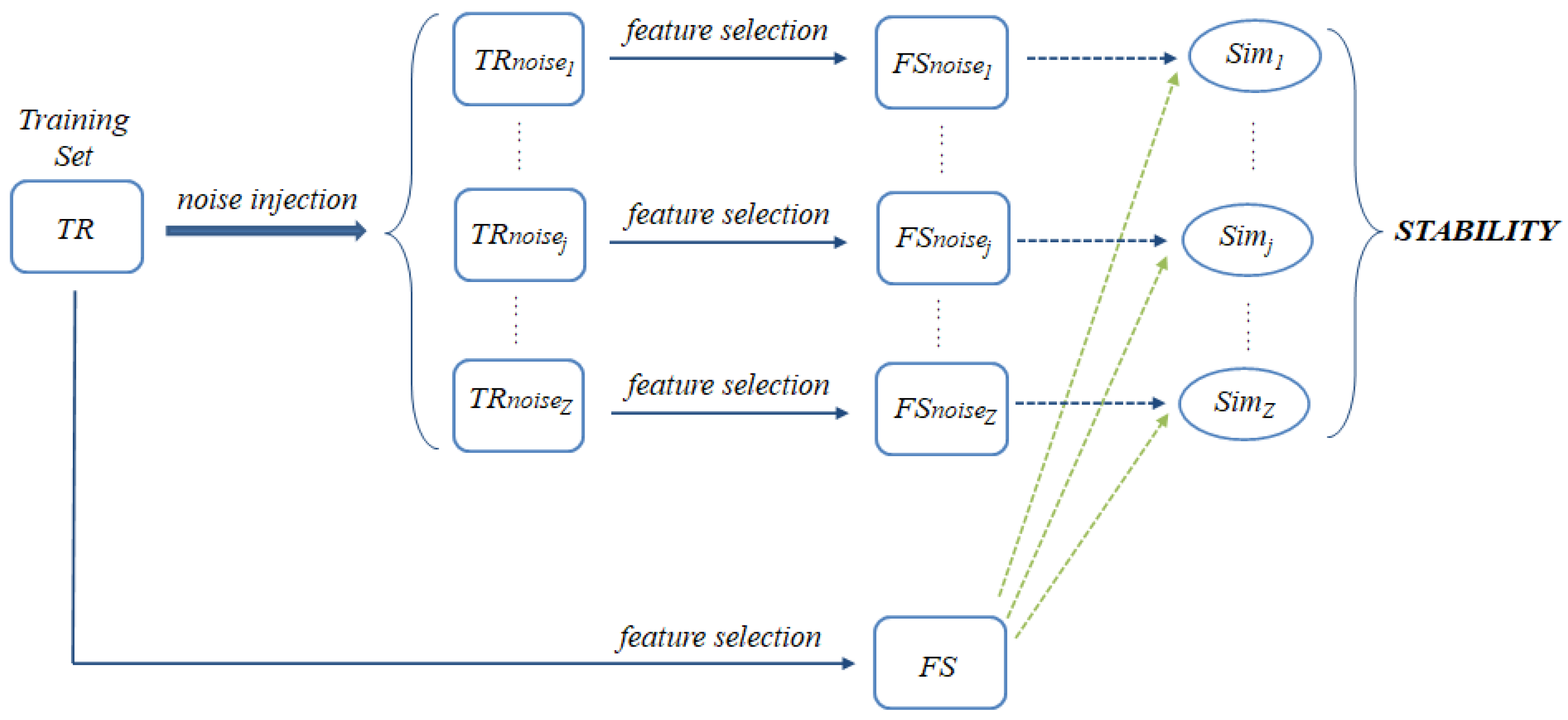
Regardless of the specific algorithm adopted for feature selection, the methodology used to evaluate the impact of noise on the selected feature subsets and on the overall learning process involves the following steps.

• The original training data ($TR$) are perturbed according to the noise injection mechanism described in Section 3.1. Being such a mechanism completely random, the noise injection procedure is repeated several times (Z iterations), resulting in different perturbed training sets $TRnois{e}_j,j=1,\dots ,Z$. The considered feature selection method is then applied to the original training set $TR$ as well as to each perturbed training set $TRnois{e}_j$, as shown in Figure 1. The feature subset selected from the original and the perturbed data are denoted, respectively, as $FS$ and $FSnois{e}_j,j=1,\dots ,Z$.
• To evaluate the impact of noise on the composition of the selected subsets, a proper consistency index is applied to compute the similarity [34] between each $FSnois{e}_j$ and $FS$, resulting in Z similarity scores $Si{m}_j,j=1,\dots ,Z$, which are finally averaged to obtain an overall stability measure: the more similar the selection outcome obtained with and without noise injection, the more stable (robust) the selection process.
• Finally, to also evaluate the impact of noise on the final classification performance, a suitable learning algorithm is applied to the original training data $TR$, filtered to retain only the features in $FS$, as well as to each perturbed training set $TRnois{e}_j$, in turn, filtered to retain only the features in $FSnois{e}_j$. The induced models are evaluated on the same noise-free test set $TS$ in order to compare the resulting performance (see Figure 2). Specifically, the average performance over the Z noise injection iterations is measured: the more similar it is to the performance without noise, the lower the overall impact of noise on the learning process.

The methodology detailed above is meant to be general enough to be implemented with different selection algorithms and different classifiers. The specific methods included in our experimental study are introduced in the next section.

4. Materials and Methods

All materials and methods involved in our investigation are presented in the following, including the metrics used for evaluating the impact of noise in terms of selection stability and predictive performance (see Section 4.1), as well as the algorithms and datasets chosen for the experiments (see Section 4.2 and Section 4.3, respectively).

4.1. Stability and Performance Metrics

Evaluating the robustness of the feature selection process, as schematized in Figure 1, involves comparing the feature subsets obtained after noise injection ($FSnois{e}_j,j=1,\dots ,Z$) with the one ($FS$) selected from the original training data. For such a comparison, we leveraged the Kuncheva measure [35], which has proved to be a suitable choice for high-dimensional datasets such as those considered in this study. More precisely, a similarity score is computed as follows:

$$Si{m}_j=\frac{|FS\cap FSnois{e}_j|-n^2/N}{n-n^2/N}$$

(1)

where $|FS\cap FSnois{e}_j|$ is the number of features common to $FS$, and $FSnois{e}_j$, N represents the dimensionality of the data at hand, i.e., the original number of features, and n is the cardinality of the selected subsets (note that the experimental analysis was performed for feature subsets of different cardinalities, as detailed later in Section 5). Essentially, $Si{m}_j$ expresses the amount of overlap between the compared subsets, properly corrected by the probability that a feature is included in both subsets simply by chance (this probability grows as n approaches N). The overall stability of the selection process is then obtained as

$$Stability=\frac{1}{Z}\sum _{j=1}^{Z}Si{m}_j$$

(2)

i.e., as the average similarity across the Z noise injection iterations.

On the other hand, to evaluate the impact of noise injection on the quality of the selected subsets, i.e., on their ability to produce good classification models, we employed a well-known metric, namely the F-measure, widely used in the presence of imbalanced data distributions:

$$F\text{-}measure=\frac{2·precision·recall}{precision+recall}$$

(3)

where the recall (sensitivity) represents the rate of true positives, i.e., the fraction of positive instances classified correctly, while the precision represents the fraction of instances that are actually positive among those classified as positive.

More precisely, as schematized in Figure 2, we compared the average F-measure computed over Z iterations of noise injections with that obtained without data perturbation.

4.2. Selection and Classification Methods

As previously introduced in Section 1, the feature selection adopted in this study involves decreasing the number of features by choosing a subset of them following a ranking strategy.

A large variety of feature selection methods have been proposed and discussed in the literature [1], exploiting different search strategies to build candidate solutions as well as different heuristics to evaluate them. In this paper, we focus on a simple yet effective, ranking-based approach that is commonly employed when the dimensionality of the problem makes the use of more sophisticated techniques infeasible. Basically, we build a ranking of the N original features by ordering them based on their predictive power, as measured by a suitable relevance criterion; then, a subset containing the n top-ranked features is selected. Note that, if needed, this subset can be further refined through wrapper approaches that make a fine selection tuned to a specific classifier [36,37] (and which often require a preliminary dimensionality reduction due to their computational cost).

Specifically, we experimented with different criteria to rank the features, both univariate approaches that assign a relevance score to each feature, independently of the others, and multivariate approaches that also consider the inter-dependencies among the features to derive the final ranking.

Among the univariate approaches, we chose:

• Pearson’s Correlation (Correl): evaluates the importance of each feature by measuring its linear correlation with the target class [38]. The stronger the correlation, the more relevant the feature is for prediction. More in detail, it is defined as:

  $$\rho (X,Y)=\frac{{\sigma }_{XY}}{{\sigma }_X{\sigma }_Y}$$

  (4)

  where X is a generic feature, Y is the class label, ${\sigma }_{XY}$ is the covariance of X and Y while ${\sigma }_X$ and ${\sigma }_Y$ are, respectively, the standard deviations of X and Y.
• Information Gain (InfoG): assesses the extent to which we can reduce the entropy of the class (i.e., the degree of uncertainty about its prediction) by observing the value of a given feature [39]:

  $$InfoG\left(X\right)=H\left(Y\right)-H\left(Y\right|X)$$

  (5)

  where $H\left(Y\right)$ and $H\left(Y\right|X)$ represent the entropy of the class Y before and after observing the feature X, respectively.
• Gain Ratio (GainR): basically, this is a variant of InfoG that attempts to compensate for its inherent tendency to favor features with more values [39]. Specifically, the InfoG definition is changed as follows:

  $$GainR\left(X\right)=\frac{InfoG\left(X\right)}{SplitInfo\left(X\right)}$$

  (6)

  i.e., through a normalization factor expressing how broadly X splits the data:

  $$SplitInfo\left(X\right)=-\sum _{i=1}^r\frac{|X_i|}{R}lo{g}_2\frac{|X_i|}{R}$$

  (7)

  where $|X_i|$ is the number of instances in which X assumes the value $X_i$, r is the number of distinct values of X, and R is the total number of training instances.
• One Rule (OneR): is a representative of embedded feature selection methods [40], which exploit a classifier to derive a relevance score for the features. Basically, for each feature in the training data, a one-level decision tree is generated based on that feature: this involves creating a simple classification rule by determining the majority class for each feature value. The accuracy of each rule is then computed, and the features are ranked based on the quality of the corresponding rules.
  Furthermore, among the multivariate approaches, we considered the following:
• ReliefF: evaluates the relevance of the features based on their ability to distinguish between data instances that are close to each other [41]. More in detail, the algorithm iteratively draws a sample instance $R_i$ from the training set in a repeated process, as per its original two-class formulation. Then, its nearest neighbors are considered, one from the same class (nearest hit H) and one from the opposite class (nearest miss M). For each feature X, a weight $W\left(X\right)$ is then computed as follows:

  $$W\left(X\right)=\sum _{i=1}^m\left[\frac{diff(X,R_i,M)}{m}-\frac{diff(X,R_i,H)}{m}\right]$$

  (8)

  where m is the number of sample instances considered (which may coincide with the size of the training set), while $diff(X,R_i,M)$ represents the difference between the values of X in $R_i$ and M, and $diff(X,R_i,H)$ is the difference computed for $R_i$ and H. The rationale is that “good” features should have the same value for instances that belong to the same class and different values for instances of different classes.
• SVM-AW: exploits a linear SVM classifier to assign a weight to each feature, thus relying on the embedded feature selection paradigm [42]. In particular, a feature $X_j$ is ranked based on the weight $w_j$ given to the feature in the hyperplane function induced by the classifier:

  $$f\left(\mathit{X}\right)=\mathit{w}·\mathit{X}+b$$

  (9)

  where $\mathit{X}=(X_1,\dots ,X_N)$ is the N-dimensional feature vector, b is a bias constant, and $\mathit{w}=(w_1,\dots ,w_N)$ is the weight vector (note that the absolute value of each weight, AW, is considered for feature ranking).
• SVM-RFE: also uses a linear SVM classifier to assign a weight to the features but adopts a recursive feature elimination (RFE) strategy that consists of removing the features with the lowest weights and repeating the evaluation on the remaining features, as originally proposed in [43]. The ranking process involves multiple iterations, in each of which a fixed percentage p of features is removed: the lower p, the higher the computational cost of the method (since more iterations occur). Given the high dimensionality of the datasets involved in our analysis, we set $p=50\%$ to keep the computational cost contained.

In this field of study, all of the aforementioned feature selection techniques are widely used. Correlation, Information Gain, Gain Ratio, One Rule, ReliefF, and SVM-RFE in particular, were chosen with the importance of these methods to the state of the art [27,28,29,30]. We also chose to introduce the SVM-AW method in order to conduct a thorough examination. As mentioned in Section 3.1, the stability analysis included a study on the predictive performance. Random Forest is an ensemble classifier obtained by the bagging of decision trees [44]. In particular, the construction of each tree involves using diverse training data, which is derived by partitioning the original training set using the bootstrap algorithm, i.e., an approach for resampling with replacement. As highlighted in the work of Breiman et al. [44], utilizing an ensemble of multiple trees yields superior performance compared to relying on a single decision tree. Regarding the classification process, each decision tree produces its own class prediction. The model’s final prediction is determined by selecting the class that is most frequently predicted across the ensemble of trees.

4.3. Datasets

For our experiments, we chose eight high-dimensional datasets from different benchmarks, which characteristics are summarized in

Table 1. Datasets used in this study. The table lists their names, the number of features and instances, and their respective types.

Datasets	Number of Features	Number of Instances	Type of Datasets
Earn	9499	12,897	text categorization
Acq	7494	12,897	text categorization
Money	7756	12,897	text categorization
Leukemia	7129	72	microarray
Lymphoma	7129	77	microarray
Lung	7129	96	microarray
Ovarian	15,155	253	proteomics
Lsvt	310	126	biomedical

. In particular, the renowned Reuters-21,578 corpus serves as a prominent benchmark in the field of text categorization, and it encompasses datasets such as Earning and Earnings Forecasts (Earn), Mergers/Acquisitions (Acq), and Money/Foreign Exchange (Money). These datasets are utilized for the automatic assignment of predefined categories or labels to textual documents based on their content.

In the domain of genomics research, we chose three microarray datasets Leukemia [45], DLBCL Tumor (Lymphoma) [46] and Lung Cancer (Lung) [47], which comprise gene expression data obtained from experiments conducted using microarray technology.

The dataset Ovarian-Cancer (Ovarian) [48] consists of proteomic spectra obtained through mass spectrometry, enabling the identification of distinctive proteomic patterns in serum that differentiate between ovarian cancer and non-cancerous conditions.

Lastly, the LSVT Voice Rehabilitation (LSVT) dataset was the result of a study conducted on patients with Parkinson’s disease [49]. This dataset is employed to assess the effectiveness and the level of acceptability of vocal rehabilitation treatment.

5. Experimental Analysis

This section describes the experimental investigation, following the methodology outlined in Section 3. We aimed to examine the stability of the feature selection techniques described in Section 4.2 when applied to datasets subjected to varying degrees of perturbation. The experimental setup is outlined in Section 5.2, while Section 5.3, Section 5.4 and Section 5.5 present and describe the results obtained on the different dataset types. Finally, a discussion is drawn in Section 5.6.

5.1. Methodological Implementation

The experiments were conducted with the packages available in the WEKA machine learning workbench [50]. Specifically, we utilized the packages for the implementation of feature selection methods, dataset sampling, attributes filter, and classification algorithm. Due to the WEKA versatility, we were able to create a customized software package to overcome the limitations of WEKA in handling all the specified methodology phases mentioned in Section 3. Specifically, our software package focuses on three main aspects:

• The implementation of an algorithm to introduce perturbations in the training set;
• The creation of procedures for applying iterative protocols such as simple holdout, repeated holdout, and cross-validation;
• The implementation of methods to calculate and generate output for stability and performance measures.

This package was created in the Eclipse (https://www.eclipse.org/ide/, accessed on 31 July 2023) environment using the JAVA (https://www.java.com/) programming language.

5.2. Settings

The experimental settings in our work varied depending on the benchmark datasets.

Text categorization. We opted to solely use the univariate feature selection methods (Correlation, Information Gain, Gain Ratio, and One Rule) for the text categorization datasets (Earn, Acq, and Money) because of their lower computational cost and wide use within this benchmark [51].

To evaluate stability, we examined different thresholds ranging from 0.5% to 10%. However, when analyzing performance, we only considered 1% of the original features, as the datasets in this benchmark had a large number of attributes.

In the case of these datasets, it is common practice to use a standard dataset split into training and test sets. Therefore, we chose the simple holdout experimental protocol, which uses only one set each for training and testing. Due to the large number of instances in these datasets, repetition is unnecessary. Specifically, we performed a ModApte split [52], which is a common practice in the field of text categorization. More details in

Table 2. Datasets ModApte split for the text categorization benchmark.

Datasets	Number of Total Instances	Number of Training Instances	Number of Test Instances
Earn	12,897	9598	3299
Acq	12,897	9598	3299
Money	12,897	9598	3299

.

We followed a protocol involving five rounds of noise injection, with two rumor levels introduced: 10% and 20%. In our implementation, we referred to the percentage of positive instances that needed to be perturbed in the training set as $noiseP$. At the same time, the term $noiseT$ represented the overall perturbation level in the dataset. These perturbation levels were selected based on the typical percentage of noise found in datasets. It is important to note that the degree of class imbalance affects the overall perturbation level when the same noise level is applied to the positive class. In datasets with higher imbalance, where the number of positive instances is lower than the negatives, the overall noise level (noiseT) is consequently lower. The total degree of perturbation for each dataset from this benchmark is documented in

Table 3. Number of instances and perturbation levels for each dataset of the text categorization benchmark.

Datasets	Number of Instances (Training Set)	Number of Positive Instances (Training Set)	noiseP	noiseT
Earn	9598	2877	10% 20%	6% 12%
Acq	9598	1650	10% 20%	3.5% 7%
Money	9598	538	10% 20%	1% 2%

.

Microarray. A distinctive characteristic of microarray datasets is the presence of a limited number of instances in a high-dimensionality space. To address this condition, it is essential to use a repeated evaluation protocol.

For the purpose of this work, we employed a 5-fold cross-validation protocol (80% of instances for the training set and 20% for the test) and conducted five iterations of noise injection with noise levels of 10% and 20% for each training set. Analogously with Table 3,

Table 4. Number of instances and perturbation levels for each dataset of the microarray benchmark.

Datasets	Number of Instances (Training Set)	Number of Positive Instances (Training Set)	noiseP	noiseT
Leukemia	57	20	10% 20%	7% 14%
Lymphoma	61	15	10% 20%	6% 10%
Lung	76	8	10% 20%	2.5% 5%

shows how the level of total perturbation in each dataset depends on the level of class imbalance. Instead,

Table 5. 5-fold dataset split for the microarray benchmark.

Datasets	Number of Total Instances	Number of Training Instances	Number of Test Instances
Leukemia	72	57	15
Lymphoma	77	61	16
Lung	96	76	20

shows the datasets split.

In this benchmark, we employed a total of seven feature selection methods, including four univariate approaches (Information Gain, Correlation, Gain Ratio and One Rule) and three multivariate approaches (ReliefF, SVM-AW, SVM-RFE).

Consistent with the previous benchmark, the stability analysis in this study involved thresholds ranging from 0.5% to 10% for feature selection. Similarly, for the performance analysis, we focused on feature selection subsets comprising 1% of the original features.

Others. Despite the intrinsic diversity of the remaining two datasets (Ovarian and LSVT), we utilized the same settings adopted for the microarray datasets due to the small number of instances in relation to the number of features. However, because the LSVT dataset has fewer features than the other datasets, we had to select 2% of the original features for the performance tests to ensure sufficient coverage and to avoid performance degradation, as empirically evaluated.

Table 6. Number of instances and perturbation levels for each dataset of the other benchmark.

Datasets	Number of Instances (Training Set)	Number of Positive Instances (Training Set)	noiseP	noiseT
Ovarian	201	72	10% 20%	7% 14%
LSVT	100	33	10% 20%	6% 13%

illustrates each dataset’s total perturbation level, while

Table 7. 5-fold dataset split for the “others” benchmark.

Datasets	Number of Total Instances	Number of Training Instances	Number of Test Instances
Ovarian	253	201	52
LSVT	126	100	26

shows the datasets split.

5.3. Results on Text Categorization Datasets

Stability results. The results in terms of stability are summarized in Figure 3.

In the case of the Earn dataset, it is evident that the feature selection methods of Correlation and Information Gain exhibit the highest stability, and Gain Ratio and One Rule have the worst stability of all the approaches. Notably, One Rule demonstrates good stability at smaller thresholds, while Gain Ratio does not. However, this behavior reverses with larger thresholds, where Gain Ratio becomes more stable than One Rule. It is worth noting that the robustness of One Rule tends to decrease as the number of selected features increases.

Considering the dataset Acq, the previously made observations are reaffirmed apart from minor fluctuations. Correlation and Information Gain consistently exhibit a high level of stability. In contrast, the behavior of Gain Ratio and One Rule remains unvaried. The observed trend from previous cases is also confirmed in the Money dataset.

After taking into account all the considerations mentioned above, a clear pattern can be extrapolated from this benchmark. In particular, both Correlation and Information Gain exhibit almost identical stability curves for the two levels of perturbation (10% and 20%), indicating a consistent and reliable response in terms of stability. As previously mentioned, Gain Ratio and One Rule methods are more sensitive to increasing perturbation, with significantly different values for very low thresholds (<5%).

Performance results. 

Table 8. The analysis of the text categorization benchmark using the Random Forest classifier produced results at varying noise levels, with the F-Measure as the evaluation metric. The subsets were created by selecting 1% of the original set of features using four different feature selection techniques (Correl, InfoG, GainR, OneR) and compared with the results obtained without feature selection (NO FS).

Dataset	1% of Features	NO FS	Correl	InfoG	GainR	OneR
Earn	clean	0.96	0.98	0.97	0.96	0.97
	noiseP = 10% (noiseT = 6%)	0.96	0.97	0.97	0.95	0.96
	noiseP = 20% (noiseT = 12%)	0.95	0.94	0.95	0.94	0.93
Acq	clean	0.84	0.86	0.86	0.77	0.80
	noiseP = 10% (noiseT = 3.5%)	0.74	0.83	0.83	0.51	0.77
	noiseP = 20% (noiseT = 7%)	0.58	0.78	0.79	0.17	0.70
Money	clean	0.36	0.62	0.66	0.33	0.49
	noiseP = 10% (noiseT = 1%)	0.33	0.56	0.60	0.17	0.41
	noiseP = 20% (noiseT = 2%)	0.28	0.49	0.54	0.13	0.32

summarizes the performance achieved in the experiments. The metric used to evaluate the model’s effectiveness is the F-measure.

Analyzing the Earn dataset results, the noise influences high performance in a contained way. Indeed, the F-measure values are not inferior to 0.93. Notice that with the Information Gain, there are no differences between the selector’s performances when applied to the clean and the perturbed dataset with $noiseP=10\%$. The other cases have minimal variations in the F-measure values (max 0.04). Correlation and Information Gain are the feature selection methods with the best performances, which confirms their good stability shown in Figure 3.

The aforementioned selectors demonstrate efficiency even when applied to the Acq dataset. However, there is a slight degradation in the performance of the One Rule selector and a substantial decline in the performance of the Gain Ratio, which reaches an F-measure value of 0.17 where the dataset is perturbed with $noiseP=20\%$.

The class imbalance of Money dataset led to degraded performance for all feature selectors. In this case, too, Correlation and Information Gain resulted in the most efficient selectors while Gain Ratio had the worst performances.

To sum up, the feature selection methods Correlation and Information Gain have strong stability with good performance and are minimally affected by the presence of noise. The stability of One Rule is notable at lower thresholds; however, its performances may not be satisfactory in specific classification contexts, such as for the Money dataset where the F-measure value arrives at 0.41. In addition, Gain Ratio is susceptible to noise with low thresholds, especially with Acq and Money datasets where it has an F-measure value inferior to 0.20.

5.4. Results on Microarray Datasets

Stability results. The stability of the selected feature selection methods in this benchmark is depicted in Figure 4.

Among the univariate approaches, Correlation demonstrates the highest stability, although its results do not match those of the text categorization benchmark. Information Gain exhibits good stability, comparable to Correlation, particularly at lower thresholds and with less imbalanced datasets such as Leukemia and Lymphoma. Alternatively, the stability of the Gain Ratio and One Rule varies depending on the dataset, generally yielding lower results.

Regarding multivariate feature selection, ReliefF is the most robust. In contrast, SVM-AW and SVM-RFE obtained the worst stability, consistently scoring below 0.4 on the Kuncheva index.

Performance results. The results of the experiments are summarized in

Table 9. The analysis of the microarray benchmark using the Random Forest classifier produced results at varying noise levels, with the F-Measure as the evaluation metric. The subsets were created by selecting 1% of the original set of features using seven different feature selection techniques (Correl, InfoG, GainR, OneR, SVM-AW, SVM-RFE, and ReliefF) and compared with the results obtained without feature selection (NO FS).

Dataset	1% of Features	NO FS	Correl	InfoG	GainR	OneR	SVM-AW	SVM-RFE	ReliefF
Leukemia	clean	0.78	0.94	0.91	0.96	0.91	0.89	0.95	0.96
	noiseP = 10% (noiseT = 7%)	0.70	0.91	0.92	0.90	0.93	0.86	0.87	0.90
	noiseP = 20% (noiseT = 14%)	0.63	0.86	0.87	0.82	0.81	0.59	0.78	0.85
Lymphoma	clean	0.47	0.83	0.70	0.75	0.74	0.84	0.91	0.78
	noiseP = 10% (noiseT = 6%)	0.34	0.75	0.63	0.56	0.66	0.55	0.66	0.73
	noiseP = 20% (noiseT = 10%)	0.25	0.71	0.62	0.49	0.46	0.44	0.42	0.72
Lung-cancer	clean	0.67	1.00	1.00	1.00	1.00	0.93	0.93	1.00
	noiseP = 10% (noiseT = 2.5%)	0.51	0.93	0.91	0.84	0.88	0.74	0.80	0.94
	noiseP = 20% (noiseT = 5%)	0.13	0.81	0.87	0.74	0.85	0.48	0.59	0.85

, where the performance of the models is evaluated using the F-measure metric.

When analyzing the Leukemia dataset, it is observed that the performances of the feature selection methods applied to the clean dataset and the noise dataset do not exhibit a significant difference. The presence of perturbances significantly affected the performance of the Gain Ratio, SVM-AW, and SVM-RFE selectors. With a noise level of 20%, they underwent considerable performance degradation. For example, SVM-AW achieved an F-measure value of 0.59 with noise, much lower than the value of 0.89 obtained without any noise.

Considering the Lymphoma dataset, the noise impact can be observed on the less stable feature selection methods, such as Gain Ratio and One Rule for univariate methods, as well as SVM-AW and SVM-RFE for multivariate methods.

The perturbations heavily influence the performance with the Lung dataset, particularly the SVM-based selectors. In conclusion, we can state that in this domain, Correlation, Information Gain, and ReliefF demonstrate consistent performance even in the presence of noises.

5.5. Results on Others Dataset

Stability results. The stability trends of the last two datasets can be observed in Figure 5. Due to the different nature of these datasets, the stability tendencies also differ.

For the Ovarian dataset, similar considerations can be made as for the microarray benchmark. Specifically, among the univariate methods, Correlation exhibits the highest level of robustness across all considered thresholds. ReliefF emerges as the most stable method when considering the multivariate approaches, while the SVM-based methods demonstrate the lowest stability.

Regarding the results obtained with the LSVT dataset, fluctuations are observed depending on the number of selected features. Overall, Correlation and ReliefF are the most robust methods in this context. Nevertheless, One Rule and the SVM-based selectors are the most vulnerable for all thresholds.

Performance results. The summarized results of the experiments conducted on the last two datasets can be found in

Table 10. The analysis of the “others” benchmark using the Random Forest classifier produced results at varying noise levels, with the F-Measure as the evaluation metric. The feature subsets of the Ovarian dataset consist of 1% of the original set of features, whereas the feature subsets of the LSVT dataset comprise 2% of the original features. For this benchmark, we used seven different feature selection techniques (Correl, InfoG, GainR, OneR, SVM-AW, SVM-RFE, and ReliefF) and compared them with the results obtained without feature selection (NO FS).

Dataset	Setting	NO FS	Correl	InfoG	GainR	OneR	SVM-AW	SVM-RFE	ReliefF
Ovarian (1% of features)	clean	0.93	0.98	0.98	0.98	0.98	0.98	0.99	0.98
	noiseP = 10% (noiseT = 7%)	0.89	0.97	0.98	0.98	0.97	0.93	0.97	0.97
	noiseP = 20% (noiseT = 14%)	0.88	0.94	0.95	0.96	0.93	0.81	0.92	0.95
LSVT (2% of features)	clean	0.77	0.70	0.64	0.60	0.77	0.63	0.71	0.75
	noiseP = 10% (noiseT = 6%)	0.72	0.70	0.66	0.58	0.66	0.59	0.68	0.66
	noiseP = 20% (noiseT = 13%)	0.63	0.64	0.60	0.55	0.61	0.52	0.58	0.66

. The evaluation of feature selection methods in combination with random forest with a clean and perturbed dataset was carried out using the F-measure metric.

The performance of the Ovarian dataset demonstrates strong results with high F-measure values. However, the impact of noise becomes apparent when using the SVM-based selectors. Indeed, the F-measure value decreases by 0.17. This result demonstrates that these selectors are unstable when employed with perturbed datasets.

For the LSVT dataset, there are no selectors superior to others; generally speaking, they all exhibit a reasonable sensitivity to noise. The One Rule and SVM-RFE selectors, which were discovered to be the most unstable, have an explicit dependency on the perturbation level.

5.6. Discussion

In this study, an extensive experimental study was conducted on three benchmarks with distinct characteristics. The datasets for text categorization have numerous instances in a high-dimensionality space, while microarray datasets exhibit a scarcity of instances described by a substantial number of features. This condition also characterizes the Ovarian dataset, framed within the “others” datasets. In the latter category, the LSVT dataset, on the other hand, has a limited number of instances and features.

We examined different levels of class balance in various contexts. We found that perturbations significantly impact feature selection, especially in situations where using a limited number of features is essential, such as in the medical field. Our research shows that selectors like the univariate One Rule and Gain Ratio, along with multivariate SVM-based methods, are highly dependent on perturbations (see Figure 4 and Table 9). These observations emphasize the need for careful consideration when using feature selection methods in scenarios where stability is crucial.

Our analysis found that the most reliable method for selecting individual features from a dataset is the Correlation. This method consistently performed well across various datasets, including Earn, Acq, Leukemia, Ovarian, and LSVT. The Information Gain method also showed good stability in these datasets.

Among the multivariate methods, ReliefF was consistently the most stable. Gain Ratio and One Rule were generally found to be less reliable than the other univariate methods. Interestingly, our study revealed that the SVM-based selectors, specifically SVM-AW and SVM-RFE, were highly sensitive to noise and therefore performed poorly in terms of stability in datasets such as Lung, Leukemia, and Ovarian. Based on the experimental results, the stability of a selector is closely associated with its performance. Additionally, the level of class imbalance in a dataset affects the impact of noise on the selector. These observations suggest that a stable selector tends to exhibit better performance, and the impact of noise on this selector may vary based on the imbalance of classes in the dataset. For instance, we observed that the Correlation selector, known for its high stability, exhibited its lowest performance when applied to the Money dataset, which has the highest level of class imbalance among all the datasets in our study.

Additionally, using a selection in conjunction with a classifier is more reliable than using a classifier alone in seven of eight datasets. This condition is demonstrated clearly in the microarray benchmark. Regardless of the specific conditions or combinations, we consistently found that the classifier’s performance was always better when used in conjunction with any selector, as shown in Table 9.

6. Conclusions and Future Work

In this work, we presented an evaluation of feature selection robustness on class noisy data. We defined a methodology that examines how noise affects the composition of feature subsets and the performance of models created using those subsets. To conduct the experiments, we implemented software that enabled an extensive comparative study of different datasets based on their domain, dimensionality, instances-to-features ratio, and distribution of classes. In particular, we used three different cases of study, represented by three benchmarks (text categorization, microarray and others) for a total of 8 datasets (Earn, Acq, Money, Leukemia, Lymphoma, Lung, Ovarian, and LSVT).

Considering the results reported and discussed in Section 5.3, Section 5.4, Section 5.5 and Section 5.6, it can be deduced that specific feature selection methods exhibit natural robustness, regardless of the domain’s characteristics. In particular, the univariate methods Correlation and Information Gain, as well as the multivariate approach ReliefF, consistently demonstrate their robustness. Conversely, the performance of methods like Gain Ratio and One Rule varies depending on the dataset’s structure. Among the feature selection methods, the multivariate SVM-based selectors, namely SVM-AW and SVM-RFE, show high sensitivity to noise across all domains considered. Despite performing well without perturbations, these methods exhibit weak robustness when exposed to noise. Numerous experiments have also shown that using a selector-classifier combination offers more noise resistance than using a single classifier (i.e., trained without feature selection).

On the one hand, these results align with the few studies published in the literature on this particular topic. On the other hand, this topic still requires further research and in-depth comparative studies on a wide range of case studies. However, our study provides a new and interesting perspective by analyzing how noise affects selection stability and performance in two dimensions (selection stability and performance). The results are encouraging for dealing with high-dimensional data.

Our research has the potential for expansion in several areas. One such area is the inclusion of new feature selection methods to facilitate a more thorough analysis of different techniques’ performance. Currently, the performance evaluation of the feature selection methods with or without the presence of perturbation has been limited to a single classifier. Indeed, an important improvement regards the inclusion of multiple classifiers to broaden and enrich our research.

Additionally, it would be beneficial to explore the integration of alternative noise injection methods and different similarity metrics. This would enable a more thorough investigation of the impact of noise on feature selection by providing a broader set of perturbation techniques.

Another potential limitation concerns the examination of feature selection stability using artificial noise rather than natural noise. Nevertheless, it is essential to acknowledge that obtaining datasets containing only one type of noise, such as class noise in our study, can be challenging. Finally, to validate the patterns identified in our study, it would be useful to expand the analysis by including other datasets from various benchmarks to test the generalizability of our results and provide further robustness to the insights found in this work.

References

1. Bolón-Canedo, V.; Alonso-Betanzos, A.; Morán-Fernández, L.; Cancela, B. Feature Selection: From the Past to the Future. In Advances in Selected Artificial Intelligence Areas: World Outstanding Women in Artificial Intelligence; Springer International Publishing: Cham, Switerland, 2022; pp. 11–34. [Google Scholar] [CrossRef]
2. Gupta, S.; Gupta, A. Dealing with Noise Problem in Machine Learning Data-sets: A Systematic Review. Procedia Comput. Sci. 2019, 161, 466–474. [Google Scholar] [CrossRef]
3. García, S.; Luengo, J.; Herrera, F. Dealing with Noisy Data. In Data Preprocessing in Data Mining; Springer International Publishing: Cham, Switerland, 2015; pp. 107–145. [Google Scholar] [CrossRef]
4. Frénay, B.; Doquire, G.; Verleysen, M. Estimating mutual information for feature selection in the presence of label noise. Comput. Stat. Data Anal. 2014, 71, 832–848. [Google Scholar] [CrossRef]
5. Wald, R.; Khoshgoftaar, T.M.; Shanab, A.A. The effect of measurement approach and noise level on gene selection stability. In Proceedings of the 2012 IEEE International Conference on Bioinformatics and Biomedicine, Philadelphia, PA, USA, 4–7 October 2012; pp. 1–5. [Google Scholar] [CrossRef]
6. Saseendran, A.; Setia, L.; Chhabria, V.; Chakraborty, D.; Barman Roy, A. Impact of Noise in Dataset on Machine Learning Algorithms. Mach. Learn. Res. 2019; early-review. [Google Scholar] [CrossRef]
7. Shanthini, A.; Vinodhini, G.; Chandrasekaran, R.M.; Supraja, P. A taxonomy on impact of label noise and feature noise using machine learning techniques. Soft Comput. 2019, 23, 8597–8607. [Google Scholar] [CrossRef]
8. Fawzi, A.; Moosavi-Dezfooli, S.M.; Frossard, P. Robustness of Classifiers: From Adversarial to Random Noise. Adv. Neural Inf. Process. Syst. 2016, 29, 1632–1640. [Google Scholar]
9. Anyfantis, D.; Karagiannopoulos, M.; Kotsiantis, S.; Pintelas, P. Robustness of learning techniques in handling class noise in imbalanced datasets. In Artificial Intelligence and Innovations 2007: From Theory to Applications; Springer: Boston, MA, USA, 2007; Volume 247, pp. 21–28. [Google Scholar] [CrossRef] [Green Version]
10. Frenay, B.; Verleysen, M. Classification in the Presence of Label Noise: A Survey. IEEE Trans. Neural Netw. Learn. Syst. 2014, 25, 845–869. [Google Scholar] [CrossRef]
11. Bolón-Canedo, V.; Sánchez-Maroño, N.; Alonso-Betanzos, A. A review of feature selection methods on synthetic data. Knowl. Inf. Syst. 2013, 34, 483–519. [Google Scholar] [CrossRef]
12. Nogueira, S.; Sechidis, K.; Brown, G. On the Stability of Feature Selection Algorithms. J. Mach. Learn. Res. 2018, 18, 1–54. [Google Scholar]
13. Altidor, W.; Khoshgoftaar, T.M.; Napolitano, A. A noise-based stability evaluation of threshold-based feature selection techniques. In Proceedings of the 2011 IEEE International Conference on Information Reuse & Integration, Las Vegas, NV, USA, 3–5 August 2011; pp. 240–245. [Google Scholar] [CrossRef]
14. Pes, B. Evaluating Feature Selection Robustness on High-Dimensional Data. In Hybrid Artificial Intelligence Systems; Springer: Boston, MA, USA, 2018. [Google Scholar]
15. Gamberger, D.; Lavrac, N.; Džeroski, S. Noise Detection and Elimination in data Preprocessing: Experiments in Medical Domains. Appl. Artif. Intell. 2000, 14, 205–223. [Google Scholar] [CrossRef]
16. Sánchez, J.; Barandela, R.; Marqués, A.; Alejo, R.; Badenas, J. Analysis of new techniques to obtain quality training sets. Pattern Recognit. Lett. 2003, 24, 1015–1022. [Google Scholar] [CrossRef]
17. Zhu, X.; Wu, X.; Yang, Y. Error Detection and Impact-Sensitive Instance Ranking in Noisy Datasets. Proc. Natl. Conf. Artif. Intell. 2004, 1, 378–384. [Google Scholar]
18. Kim, S.; Zhang, H.; Wu, R.; Gong, L. Dealing with noise in defect prediction. In Proceedings of the 2011 33rd International Conference on Software Engineering (ICSE), Honolulu, HI, USA, 21–28 May 2011; pp. 481–490. [Google Scholar] [CrossRef]
19. Van Hulse, J.; Khoshgoftaar, T. Knowledge discovery from imbalanced and noisy data. Data & Knowl. Eng. 2009, 68, 1513–1542. [Google Scholar] [CrossRef]
20. Nettleton, D.F.; Orriols-Puig, A.; Fornells, A. A study of the effect of different types of noise on the precision of supervised learning techniques. Artif. Intell. Rev. 2010, 33, 275–306. [Google Scholar] [CrossRef]
21. Johnson, J.M.; Khoshgoftaar, T.M. A Survey on Classifying Big Data with Label Noise. J. Data Inf. Qual. 2022, 14, 1–43. [Google Scholar] [CrossRef]
22. He, S.; Chen, H.; Zhu, Z.; Ward, D.G.; Cooper, H.J.; Viant, M.R.; Heath, J.K.; Yao, X. Robust twin boosting for feature selection from high-dimensional omics data with label noise. Inf. Sci. 2015, 291, 1–18. [Google Scholar] [CrossRef]
23. Zhang, W.; Rekaya, R.; Bertrand, K. A method for predicting disease subtypes in presence of misclassification among training samples using gene expression: Application to human breast cancer. Bioinformatics 2006, 22, 317–325. [Google Scholar] [CrossRef] [Green Version]
24. Abu Shanab, A.; Khoshgoftaar, T. Filter-Based Subset Selection for Easy, Moderate, and Hard Bioinformatics Data. In Proceedings of the 2018 IEEE International Conference on Information Reuse and Integration (IRI), Salt Lake City, UT, USA, 6–9 July 2018; pp. 372–377. [Google Scholar] [CrossRef]
25. Pes, B. Feature Selection for High-Dimensional Data: The Issue of Stability. In Proceedings of the 2017 IEEE 26th International Conference on Enabling Technologies: Infrastructure for Collaborative Enterprises (WETICE), Poznan, Poland, 21–23 June 2017; pp. 170–175. [Google Scholar] [CrossRef]
26. Khaire, U.M.; Dhanalakshmi, R. Stability of feature selection algorithm: A review. J. King Saud Univ.-Comput. Inf. Sci. 2022, 34, 1060–1073. [Google Scholar] [CrossRef]
27. Li, F.; Mi, H.; Yang, F. Exploring the stability of feature selection for imbalanced intrusion detection data. In Proceedings of the 2011 9th IEEE International Conference on Control and Automation (ICCA), Santiago, Chile, 19–21 December 2011; pp. 750–754. [Google Scholar] [CrossRef]
28. Dessì, N.; Pes, B. Stability in Biomarker Discovery: Does Ensemble Feature Selection Really Help? In Proceedings of the Current Approaches in Applied Artificial Intelligence; Springer International Publishing: Cham, Switerland, 2015; pp. 191–200. [Google Scholar]
29. Dessì, N.; Pes, B.; Angioni, M. On Stability of Ensemble Gene Selection. In Proceedings of the Intelligent Data Engineering and Automated Learning—IDEAL 2015; Springer International Publishing: Cham, Switerland, 2015; pp. 416–423. [Google Scholar]
30. Wang, H.; Khoshgoftaar, T.M.; Seliya, N. On the Stability of Feature Selection Methods in Software Quality Prediction: An Empirical Investigation. Int. J. Softw. Eng. Knowl. Eng. 2015, 25, 1467–1490. [Google Scholar] [CrossRef]
31. Jiang, L.; Haiminen, N.; Carrieri, A.P.; Huang, S.; Vázquez-Baeza, Y.; Parida, L.; Kim, H.C.; Swafford, A.D.; Knight, R.; Natarajan, L. Utilizing stability criteria in choosing feature selection methods yields reproducible results in microbiome data. Biometrics 2022, 78, 1155–1167. [Google Scholar] [CrossRef]
32. Manca, M.M.; Pes, B.; Riboni, D. Exploiting Feature Selection in Human Activity Recognition: Methodological Insights and Empirical Results Using Mobile Sensor Data. IEEE Access 2022, 10, 64043–64058. [Google Scholar] [CrossRef]
33. Zhu, X.; Wu, X. Cost-guided class noise handling for effective cost-sensitive learning. In Proceedings of the Fourth IEEE International Conference on Data Mining (ICDM’04), Brighton, UK, 1–4 November 2004; pp. 297–304. [Google Scholar] [CrossRef]
34. Cannas, L.M.; Dessì, N.; Pes, B. Assessing similarity of feature selection techniques in high-dimensional domains. Pattern Recognit. Lett. 2013, 34, 1446–1453. [Google Scholar] [CrossRef] [Green Version]
35. Kuncheva, L. A stability index for feature selection. In Proceedings of the 25th IASTED International Multi-Conference: Artificial Intelligence and Applications, Innsbruck, Austria, 12–14 February 2007; ACTA Press: Anaheim, CA, USA, 2007; pp. 390–395. [Google Scholar]
36. Almugren, N.; Alshamlan, H. A survey on hybrid feature selection methods in microarray gene expression data for cancer classification. IEEE Access 2019, 7, 78533–78548. [Google Scholar] [CrossRef]
37. Cannas, L.M.; Dessì, N.; Pes, B. A filter-based evolutionary approach for selecting features in high-dimensional micro-array data. In Intelligent Information Processing V, Proceedings of the 6th IFIP TC 12 International Conference, IIP 2010, Manchester, UK, 13–16 October 2010; Proceedings 6; Springer: Berlin/Heidelberg, Germany, 2010; pp. 297–307. [Google Scholar]
38. Tan, P.N.; Steinbach, M.; Karpatne, A.; Kumar, V. Introduction to Data Mining; Pearson: London, UK, 2019. [Google Scholar]
39. Witten, I.H.; Frank, E.; Hall, M.A.; Pal, C.J. Data Mining: Practical Machine Learning Tools and Techniques, 4th ed.; Morgan Kaufmann: San Francisco, CA, USA, 2016. [Google Scholar]
40. Dessì, N.; Pes, B. Similarity of feature selection methods: An empirical study across data intensive classification tasks. Expert Syst. Appl. 2015, 42, 4632–4642. [Google Scholar] [CrossRef]
41. Urbanowicz, R.J.; Meeker, M.; La Cava, W.; Olson, R.S.; Moore, J.H. Relief-based feature selection: Introduction and review. J. Biomed. Inform. 2018, 85, 189–203. [Google Scholar] [CrossRef]
42. Bolón-Canedo, V.; Sánchez-Maroño, N.; Alonso-Betanzos, A. Feature Selection for High-Dimensional Data; Springer: Berlin/Heidelberg, Germany, 2015. [Google Scholar]
43. Guyon, I.; Weston, J.; Barnhill, S.; Vapnik, V. Gene Selection for Cancer Classification using Support Vector Machines. Mach. Learn. 2002, 46, 389–422. [Google Scholar] [CrossRef]
44. Breiman, L. Random Forests. Mach. Learn. 2001, 45, 5–32. [Google Scholar] [CrossRef] [Green Version]
45. Golub, T.R.; Slonim, D.K.; Tamayo, P.; Huard, C.; Gaasenbeek, M.; Mesirov, J.P.; Coller, H.A.; Loh, M.L.; Downing, J.R.; Caligiuri, M.A.; et al. Molecular classification of cancer: Class discovery and class prediction by gene expression monitoring. Science 1999, 286, 531–537. [Google Scholar] [CrossRef] [Green Version]
46. Shipp, M.; Ross, K.; Tamayo, P.; Weng, A.; Kutok, J.; Aguiar, T.; Gaasenbeek, M.; Angelo, M.; Reich, M.; Pinkus, G.; et al. Diffuse large B-cell lymphoma outcome prediction by gene-expression profiling and supervised machine learning. Nat. Med. 2002, 8, 68–74. [Google Scholar] [CrossRef]
47. Beer, D.; Kardia, S.; Huang, C.; Giordano, T.; Levin, A.; Misek, D.; Lin, L.; Chen, G.; Gharib, T.; Thomas, D.; et al. Gene-expression profiles predict survival of patients with lung adenocarcinoma. Nat. Med. 2002, 8, 816–824. [Google Scholar] [CrossRef]
48. Petricoin, E.F.; Ardekani, A.M.; Hitt, B.A.; Levine, P.J.; Fusaro, V.A.; Steinberg, S.M.; Mills, G.B.; Simone, C.; Fishman, D.A.; Kohn, E.C.; et al. Use of proteomic patterns in serum to identify ovarian cancer. Lancet 2002, 359, 572–577. [Google Scholar] [CrossRef]
49. Tsanas, A.; Little, M.A.; Fox, C.; Ramig, L.O. Objective Automatic Assessment of Rehabilitative Speech Treatment in Parkinson’s Disease. IEEE Trans. Neural Syst. Rehabil. Eng. 2014, 22, 181–190. [Google Scholar] [CrossRef] [Green Version]
50. Witten, I.H.; Frank, E.; Hall, M.A.; Pal, C.J. (Eds.) Appendix B—The WEKA workbench. In Data Mining, 4th ed.; Morgan Kaufmann: San Francisco, CA, USA, 2017; pp. 553–571. [Google Scholar] [CrossRef]
51. Forman, G. An Extensive Empirical Study of Feature Selection Metrics for Text Classification. J. Mach. Learn. Res. 2003, 3, 1289–1305. [Google Scholar]
52. Debole, F.; Sebastiani, F. An Analysis of the Relative Hardness of Reuters-21578 Subsets: Research Articles. J. Am. Soc. Inf. Sci. Technol. 2005, 56, 584–596. [Google Scholar] [CrossRef] [Green Version]
Figure 1. Evaluation of feature selection stability in the presence of noise.
Information 14 00438 g001
Figure 2. Evaluation of classification performance with and without noise injection.
Information 14 00438 g002
Figure 3. Stability results obtained with different thresholds ranging from 0.5% to 10% using Correlation, Information Gain, Gain Ratio and One Rule as selectors in the text categorization benchmark.
Information 14 00438 g003
Figure 4. Stability results obtained with different thresholds ranging from 0.5% to 10% using Correlation, Information Gain, Gain Ratio, One Rule, SVM-AW, SVM-RFE and ReliefF as selectors in the microarray benchmark.
Information 14 00438 g004
Figure 5. Stability results obtained with different thresholds ranging from 0.5% to 10% using Correlation, Information Gain, Gain Ratio, One Rule, SVM-AW, SVM-RFE and ReliefF as selectors in the others benchmark.
Information 14 00438 g005