An Extensive Performance Comparison between Feature Reduction and Feature Selection Preprocessing Algorithms on Imbalanced Wide Data

Abstract

The most common preprocessing techniques used to deal with datasets having high dimensionality and a low number of instances—or wide data—are feature reduction (FR), feature selection (FS), and resampling. This study explores the use of FR and resampling techniques, expanding the limited comparisons between FR and filter FS methods in the existing literature, especially in the context of wide data. We compare the optimal outcomes from a previous comprehensive study of FS against new experiments conducted using FR methods. Two specific challenges associated with the use of FR are outlined in detail: finding FR methods that are compatible with wide data and the need for a reduction estimator of nonlinear approaches to process out-of-sample data. The experimental study compares 17 techniques, including supervised, unsupervised, linear, and nonlinear approaches, using 7 resampling strategies and 5 classifiers. The results demonstrate which configurations are optimal, according to their performance and computation time. Moreover, the best configuration—namely, k Nearest Neighbor (KNN) + the Maximal Margin Criterion (MMC) feature reducer with no resampling—is shown to outperform state-of-the-art algorithms.

1. Introduction

Within the machine learning field, the term “wide data” [1] refers to datasets containing a much greater number of features than instances. This type of data is common in bioinformatics [2,3], and usually presents two main problems that affect the performance of learning algorithms: the curse of dimensionality and data imbalance.

The curse of dimensionality [4] refers to the difficulty of accurately generalizing problems with high-dimensional datasets when using machine learning algorithms. This increases both the processing time and required space, as well as the risk of overfitting, as it makes it difficult to distinguish meaningful patterns from noise.

Considering the low number of instances, wide data are prone to imbalance caused by the large difference in the number of instances per class [5]. The algorithms trained with this data may be biased towards the majority class, making it difficult to accurately classify data belonging to the minority classes.

One of the solutions that may mitigate these problems is the use of preprocessing techniques. In particular, the curse of dimensionality can be addressed with feature selection (FS) [6] and feature reduction (FR) [7] methods. FS methods identify and select the most informative and relevant features from a given dataset, discarding the noisy or redundant data. In contrast, FR methods transform the original feature space into a lower-dimensional one using the information present in the original features.

Resampling methods [8] solve the imbalanced data problem through removing instances from the majority class or creating new ones for the minority class.

There are many application examples of these methods in different areas. For example, in medicine, FR improves the accuracy of epilepsy diagnosis through analyzing electroencephalography signals, avoiding invasive techniques [9]. FS has been also used for breast cancer detection [10] analyzing microarray data. Regarding engineering, the authors of [11] used Principal Component Analysis (PCA) in several predictors to remove noise from building energy consumption datasets. In another example, in fault diagnosis, FS was applied to select the best features extracted from magnet DC motors [12] or rotating machinery [13]. Furthermore, FR techniques are valuable in text mining tasks, such as document classification, e.g., in [14] PCA and Latent Semantic Indexing (LSI) were used to extract useful features for an SVM classifier.

This study aims to find the best strategies to process wide datasets, composed of combinations of FS or FR, resampling, and classifiers, through evaluating their performance and computation time. In the literature, studies comparing dimensionality reduction techniques with resampling methods have been limited to the use of FS [15]. In this case, new FR experiments are compared to the best results from [16], which extensively compared various FS, resampling methods, and classifiers on a wide dataset.

As mentioned in Section 2, the use of FR techniques with wide datasets requires thorough research to identify compatible approaches. For example, applying nonlinear transformations requires estimation to handle out-of-sample instances.

The scope of this study excludes the use of wrapper FS methods. As detailed in Section 3, their high computational cost is a crucial factor when processing wide data, as it presents a large number of features. Both the FS and FR algorithms used require the dimensionality to be set, which simplifies the comparison and visibility of the results, as the dimensionality can be set to be the same. The obtained results are analyzed to address the following objectives of this study:

1.

To find an FR method that is compatible with wide data and provides a means to perform nonlinear transformations over out-of-data instances.

2.

To compare the two previously mentioned types of preprocessing techniques (FR and FS) and determine which is more suitable to use on wide datasets.

3.

To determine whether balancing is important while using FR methods and, if so, whether it is more convenient to use it before or after the FR step.

4.

To determine the best FR method for each classifier.

While previous studies have included some comparisons of FS and FR algorithms over the same datasets [17], these evaluations are not particularly exhaustive. They predominantly focus on basic and widely used FR techniques, avoiding the use of nonlinear approaches. Furthermore, the lack of use of wide datasets makes it impossible to discern which techniques are optimal in such cases, as not all algorithms are compatible with such data.

Performing a large number of experiments to compare FS and FR approaches for wide datasets is one of the main novelties of this study. Due to the high presence of the imbalance problem in wide data, this study also focuses on resampling techniques in combination with FR and FS preprocessing methods. The code for all of the algorithms, allowing for their standardized use, can be found on GitHub (https://github.com/Ismael-rp/feature_reduction_feature_selection_wide_data_comparison, accessed on 15 May 2024).

The remainder of this paper is organized as follows. First, in Section 2, Section 3 and Section 4 the background for all the preprocessing methods used (i.e., FR, FS, and resampling) is provided. In Section 5, the experimental setup is detailed, while the results are shown in Section 6. Finally, the conclusions, limitations, and future work are presented in Section 7, Section 8 and Section 9, respectively. Finally, the conclusions and future work are presented in Section 7.

2. Feature Reduction

Feature reduction (FR) or manifold learning [7] methods are preprocessing techniques used to reduce the number of dimensions of high-dimensional datasets. This is useful for improving the performance of learning algorithms, enhancing data visualization, and facilitating feature extraction from images. The present study focuses on FR for wide data classification.

As previously explained, high dimensionality poses a significant challenge to classification algorithms, as it complicates the distinction between useful and noisy features. FR methods attempt to solve this problem through creating a new dataset with the desired dimensionality, combining all the original features. A good FR method should be able to determine the structure of the original dataset (manifold) and preserve it in a lower dimensional representation. This structure is divided into local and global structures. Preserving the local structure refers to preserving the distance of all individual points to their nearest neighbors, whereas the global structure refers to the rest of the further points. Preserving both structures simultaneously is difficult [18], and in FR methods, usually, only one is well retained.

There are some taxonomies that can be used to discriminate FR algorithms according to their behavior, and some of them can be very extensive, such as the one presented in the study [7]. The present manuscript divides FR methods according to two properties: supervised/unsupervised and linear/nonlinear. Unsupervised methods ignore the data labels when creating the new dataset, which makes them useful for clustering problems. On the other hand, supervised methods utilize data labels, allowing classes to be separated more effectively and, therefore, making these methods more suitable for classification problems.

Linear FR methods transform the data using a linear transformation which minimizes or maximizes some criteria and, at the same time, reduces the dimensionality as desired. As shown in Equation (1), matrix A with dimensions of $(r\times c)$ is reduced to a B matrix with k dimensions using a kernel or linear transformation K.

(1)

Non-linear transformations are required to uncover the hidden manifold in nonlinear data. As most of these algorithms are unsupervised, all of the methods used in this study are unsupervised. Unlike their linear alternatives, due to their intrinsic behavior, nonlinear methods do not provide a way to reproduce the transformation on out-of-sample data; however, the authors of [19] presented a generalized and accurate approximation to solve this issue.

Based on the fact that every point in the space is linearly relocated to a new position in the lower-dimensional space under a nonlinear transformation, this linear transformation can be approximated through the following three steps. (1) Retrieve the K out-of-sample nearest neighbor instances from the training dataset. As the authors recommend, the K value was set to 5. (2) Reduce this neighbor sub-dataset to the desired dimensionality using Principal Component Analysis (PCA). (3) Using linear regression, obtain the linear projection to transpose the neighbor sub-dataset into the final positions obtained with the FR method.

The PCA and linear regression models are applied to the out-of-sample instance to be transformed. This process is repeated for each out-of-sample instance.

Unlike traditional datasets, wide data has a much greater number of columns than rows ($r<<c$), preventing some of the most popular linear and nonlinear FR algorithms from being able to calculate the projection.

The FR methods used in this study are listed below, following the taxonomy mentioned above:

• Linear

  -

  Unsupervised

  ∗

  Principal Component Analysis (PCA) [20] is the most popular FR method, which reduces the feature dimensionality while maintaining the maximum data variance.

  ∗

  Locality Pursuit Embedding (LPE) [21] respects the local structure through maximizing the variance of each local patch according to Euclidean distances (unlike PCA, which preserves the global structure).

  ∗

  Parameter-Free Locality Preserving Projection (PFLPP) [22] is a parameter-free version of the Locality Preserving Projection (LPP) algorithm [23], which is a linear version of the nonlinear graph-based Laplacian Eigenmaps method [24].

  ∗

  Random Projection (RNDPROJ) [25] projects the data into a new random spherical hyperplane that is randomly selected using the origin. It is not a trivial computation problem.

  -

  Supervised

  ∗

  Fisher Score (FSCORE) [26] finds the projection that maximizes the ratio between each feature mean and the standard deviation of each class.

  ∗

  Locality Sensitive Laplacian Score (LSLS) [27] is based on the Laplacian score FS method [28]. It adjusts the Laplacian graph using the class label to simultaneously minimize the local within-class information and maximize the local between-class information.

  ∗

  Local Fisher Discriminant Analysis (LFDA) [29] is an improved version of the FDA-supervised FR method, which is suitable for reducing datasets in which individual classes are separated into several clusters.

  ∗

  Maximum Margin Criterion (MMC) [30] projects the data while maximizing the average margin between classes.

  ∗

  Sliced Average Variance Estimation (SAVE) [31] calculates the projection matrix by averaging the covariance of the data of each slice in which the whole dataset has been divided.

  ∗

  Supervised Locality Pursuit Embedding (SLPE) [32] is a supervised version of the LPE algorithm, which enhances the model using label data.

• Non-linear

  -

  Classical Multidimensional Scaling (MDS) [33] computes the dissimilarities between pairs of objects (assuming Euclidean distance). This matrix serves as the input for the algorithm that outputs a coordinate that minimizes a loss function called strain.

  -

  Metric Multidimensional Scaling (MMDS) [34] is a superset of the previous method. It iteratively updates the weights given by the MDS using the SMACOF algorithm, in order to minimize a stress function such as the residual sum of squares.

  -

  Locally Linear Embedding (LLE) [35] bases its performance on producing low-dimensional vectors that best reconstruct the original objects through computing the kNN and using this information to weight them.

  -

  Neighborhood Preserving Embedding (NPE) [36] first identifies the structure of the data neighborhood in the original space, then determines a linear subspace minimizing the reconstruction error of the local neighborhood structure [37].

  -

  Locally Embedded Analysis (LEA) [34] aims to preserve the local structure of the original data in the computed embedding space.

  -

  Stochastic Neighbor Embedding (SNE) [38] is a probabilistic approach that places the data in a low-dimensional space that optimally preserves the neighborhood of the original space.

  -

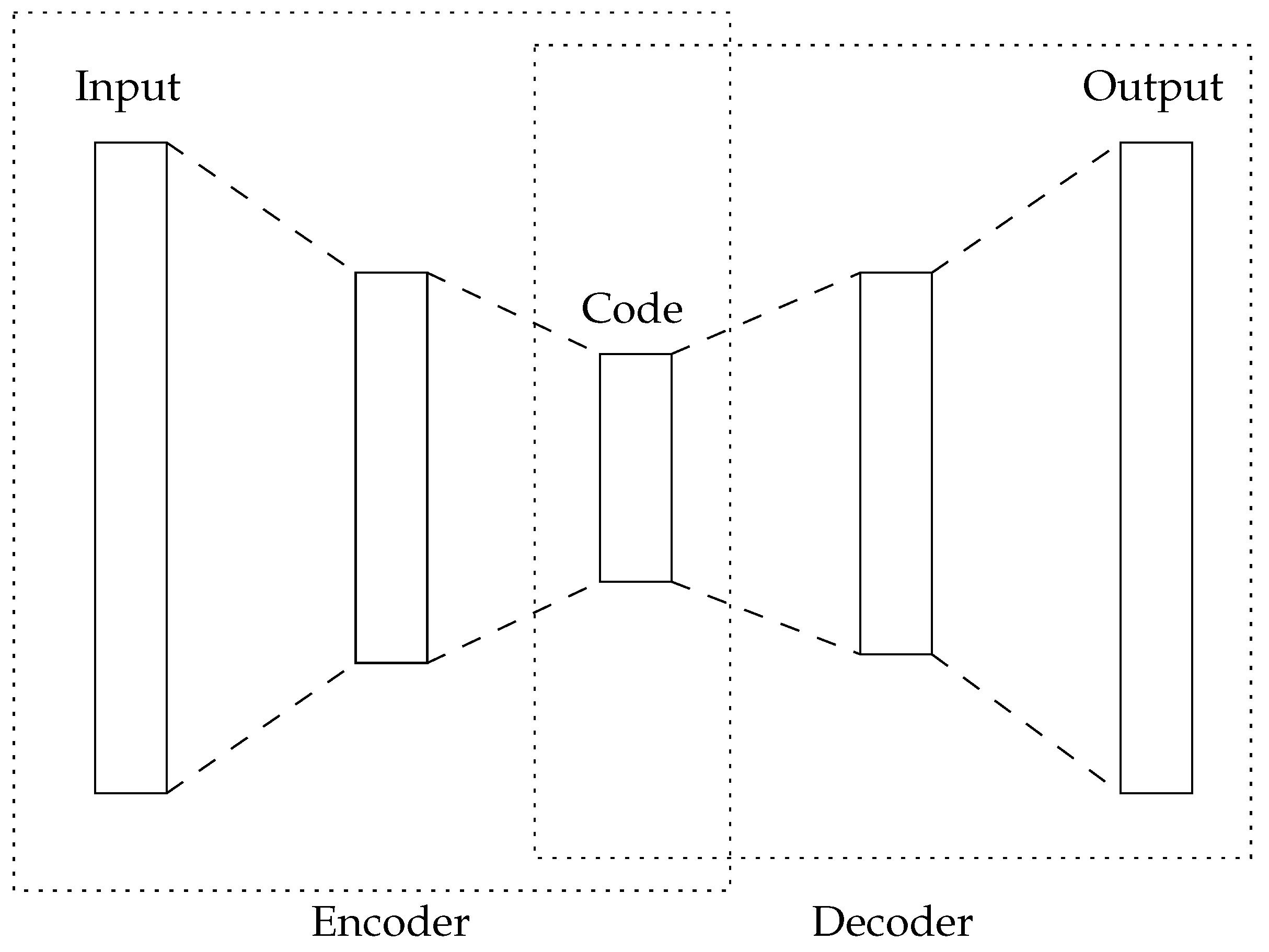
  An Autoencoder [39,40] is a kind of artificial neural network that is trained in an unsupervised manner. The aim of the autoencoder is to capture the hidden information in the high-dimensional input space of the dataset. Autoencoders have the same number of artificial neurons in their first (input) and last (output) layers, while having less in their center layers (see Figure 1). During training, Autoencoders attempt to generate the same information in the output layer that is presented in the input layer. Therefore, the center layer aims to capture the intrinsic information of the dataset and, thus, can be used for feature reduction.

3. Feature Selection

Feature selection [6] is an alternative preprocessing approach to FR, which aims to solve the curse of dimensionality. Instead of combining all features into a completely new low-dimensional dataset, FS methods identify which features are the most suitable for the classification step. These methods attempt to discard the noisy, irrelevant, and redundant features that limit the performance of the classifier.

Machine learning models that only use a few features are more interpretable than those that combine all original features into a new dataset. Generally speaking, the three types of feature selectors are filters, wrappers, and embedded:

• Filter methods [41] are mainly based on statistical measures. They analyze the features and rank them in an ordinal or numerical way according to their importance. Although these methods do not usually achieve the best performance for any classifier, they evade overfitting.
• Wrapper methods [42] perform any search algorithm to find the best feature subset for a specific classifier, according to a certain metric. Some of the most common methods are the recursive feature elimination (RFE) and genetic implementation methods. These methods obtain better performance than others; however, they tend to overfit and their computational cost is usually too high.
• Embedded methods [43] take advantage of the properties of classifiers such as support vector machines or decision trees to determine the importance of a feature subset. Although the selected subset can be used to train any model, it may perform better on the base classifier used to obtain it.

The method used for comparison with the best FR configuration is the SVM-RFE [44], the superior performance of which on wide data has been proven in a previous study [16] when compared with six of the most popular filters and embedded approaches (i.e., Ttest, Chi-squared, Random forest importance, ANOVA, Information gain, and ReliefF). SVM-RFE is an embedded FR method that recursively eliminates features according to their performance contribution, removing the feature whose associated weight in the current iteration is the minimum.

4. Imbalanced Data

There is a great chance that wide data suffer from imbalance due to the associated low number of instances. As previously stated, having a great difference in the number of instances between classes often causes a problem for the classifier [45], as its output may be biased with respect to the most-represented class. This problem can be solved through the use of any of the three types of resampling methods: removing instances from the majority class (undersampling methods), creating new instances for the minority class (oversampling methods), or combining both methods (hybrid methods).

The methods used in this study, which are the most popular ones, are described as follows:

• Random Undersampling (RUS) [46] removes instances randomly selected from the majority class.
• Random Oversampling (ROS) [46] duplicates instances randomly selected from the minority class.
• Synthetic Minority Over-sampling Technique (SMOTE) [47] creates synthetic instances of the minority class. For the creation of new instances, SMOTE randomly selects instances from the minority class. The feature values of the new instances are computed through interpolating the features of two instances randomly selected from the k nearest neighbors of the original instance (k being a parameter of the algorithm).

5. Experimental Setup

In this section, the experimental setup is explained. Some of the decisions made, such as datasets, classifiers, or balancing strategies applied, were the same as in our previous study [16].

5.1. Cross-Validation

For this study, $5\times 2$-fold cross-validation was performed, where the original dataset was randomly split into 2 parts 5 times, and each part was used for training and testing; thus, every instance was used for both training and testing 5 times.

This type of cross-validation is particularly appropriate for imbalanced data as, considering the low number of instances for some classes, performing the usual 10-fold cross-validation would leave a small number of the minority class instances on the training set [48].

5.2. Data Sets

A total of 14 wide datasets were used to compare the methods, the main characteristics of which are listed in

Table 1. Data sets used in the experimental study. Datasets 1–9 were used in [51], while 10–14 were used in [52]. The column names refer to dataset name, number of examples, number of features, ratio features/examples, minority and majority class labels, min and max percentage of instances for the minority and majority classes, and imbalance ratio. ¹ https://jundongl.github.io/scikit-feature/datasets.html, ² http://csse.szu.edu.cn/staff/zhuzx/Datasets.html, accessed on 7 April 2024.

	Data Set	#Ex.	#Feat.	$\frac{\#\mathbf{Feat}.}{\#\mathbf{Ex}.}$	Class (min.; maj.)	%min.; %maj.	IR
1	Colon 1	62	2,000	32.26	(Normal; Tumor)	0.35; 0.65	1.86
2	MLL_ALL 1	72	12,582	174.75	(ALL; rem)	0.33; 0.67	2.03
3	MLL_AML 1	72	12,582	174.75	(AML; rem)	0.39; 0.61	1.56
4	MLL_MLL 1	72	12,582	174.75	(MLL; rem)	0.28; 0.72	2.57
5	SRBCT_1 1	83	2,308	27.81	(1; rem)	0.35; 0.65	1.86
6	SRBCT_4 1	83	2,308	27.81	(4; rem)	0.30; 0.70	2.33
7	Lung_1 1	203	12,600	62.07	(rem; 1)	0.32; 0.68	2.12
8	Lung_4 1	203	12,600	62.07	(rem; 4)	0.10; 0.90	9.00
9	Lung_5 1	203	12,600	62.07	(rem; 5)	0.10; 0.90	9.00
10	Leukemia_BM 2	72	7,130	99.03	(BM; rem)	0.29; 0.71	2.45
11	TOX_171_1 2	171	5,748	33.61	(1; rem)	0.26; 0.74	2.85
12	TOX_171_2 2	171	5,748	33.61	(2; rem)	0.26; 0.74	2.85
13	TOX_171_3 2	171	5,748	33.61	(3; rem)	0.23; 0.77	3.35
14	TOX_171_4 2	171	5,748	33.61	(4; rem)	0.25; 0.75	3.00

. In addition to information commonly used in the field, we include the ratio between features and instances, due to their wide nature. All of them contained two classes and their features were numeric. Every fold from the cross-validation was standardized, setting its mean to zero and standard deviation to one. The test folds were standardized using the mean and standard deviation obtained from the training folds. The imbalance ratio [49,50] in the table was computed as the number of instances in the majority class divided by the number of instances in the minority class.

5.3. Dimensionality and Number of Features

For fairness when comparing FR and FS methods, it is appropriate to configure them to obtain datasets with the same dimensionality as the output. However, the number of features is limited in some of the nonlinear FR methods (SNE, MDS, MMDS, and LLE). Therefore, in such cases, the maximum dimensionality was set to the number of instances belonging to each fold.

5.4. Resampling Strategies

Each one of the three resampling methods detailed in Section 4 was used in two ways: (1) balancing before performing dimensionality reduction or (2) balancing after dimensionality reduction. Therefore, there were a total of seven strategies, including the option of not performing resampling.

5.5. Classifiers

According to [53], the most popular algorithms for high-dimensional data are as follows: k-nearest neighbors (KNN), SVM-Gaussian, C4.5 trees, Random Forest, and Naive Bayes. For this reason, these five classifiers were used in this study.

5.6. Parameters

After preliminary experiments involving tuning the algorithm parameters, the parameters of the algorithms were set as stated in

Table 2. All the algorithms used in the study are grouped according to their type, including their parameters (when applicable) and their corresponding R packages, all of then have been accessed on June 2023. * The asterisk indicates that, in the method, the parameter K was set to 5 in the transformation estimator needed for the nonlinear feature reducers explained in Section 2. ¹ https://cran.r-project.org/web/packages/class/index.html; ² https://cran.r-project.org/web/packages/e1071/index.html; ³ https://cran.r-project.org/web/packages/RWeka/index.html; ⁴ https://cran.r-project.org/web/packages/randomForest/randomForest.html; ⁵ https://cran.r-project.org/web/packages/naivebayes/index.html; ⁶ https://cran.r-project.org/web/packages/Rdimtools/index.html; ⁷ https://www.bioconductor.org/packages/release/bioc/html/sigFeature.html; ⁸ https://cran.r-project.org/web/packages/unbalanced/index.html, accessed on 7 April 2024.

	Algorithms	Parameters	Package
Classifier	KNN	$k=1$	class 1
	SVM-G	$c={10}^9$, $\gamma ={10}^7$	e1071 2
	C4.5	Default	RWeka 3
	Random Forest	Default	randomForest 4
	Naive Bayes	Default	naivebayes 5
Feature reduction	PCA	-	Rdimtools 6
Linear—Unsupervised	LPE	Default	Rdimtools 6
	PFLPP	-	Rdimtools 6
	RNDPROJ	Default	Rdimtools 6
Feature reduction	FSCORE	-	Rdimtools 6
Linear—Supervised	LSLS	Default	Rdimtools 6
	LFDA	Default	Rdimtools 6
	MMC	-	Rdimtools 6
	SAVE	Default	Rdimtools 6
	SLPE	-	Rdimtools 6
Feature reduction	MDS	-	Rdimtools 6
Non-linear *	MMDS	-	Rdimtools 6
	LLE	Default	Rdimtools 6
	NPE	Default	Rdimtools 6
	LEA	Default	Rdimtools 6
	SNE	Default	Rdimtools 6
	AUTOENCODER	epoch = 10, activation = “Tanh”	h2o
Feature selection	SVM-RFE		sigFeature 7
Balancing	ROS	Ratio 1:1	Own impl.
	RUS	Ratio 1:1	Own impl.
	SMOTE	Ratio 1:1, $k=5$	unbalanced 8

. This table lists all the algorithms used, as well as their corresponding parameters and implementation packages. Most parameters were set as defaults while others, such as the SVM-G classifier and SMOTE, were optimized as detailed in [16].

The SVM-G classifier was optimized using a grid parameter search, with $c={10}^9$ and $\gamma ={10}^7$, resulting in optimal performance on all datasets. For SMOTE, values of k ranging from 1 to 20 were tested, and the performance was slightly better when the recommended value of 5 was used. Regarding the balancing algorithms, the balancing ratio was set to 1 for all datasets, such that the number of instances for both the majority and minority classes was the same.

As explained in Section 2, an algorithm to approximate the transformation on out-of-sample instances on nonlinear FR is needed; this is denoted “transformation approximation” in the table and, as the authors recommended, the parameter k was set to 5. Finally, autoencoders had a single inner layer with as many neurons as the desired output dimensionality size. Several well-known functions (linear, rectilinear uniform, sigmoidal, and tangential) were considered. The tangential function learned the fastest, requiring only 10 epochs to reach the best performance on the training fold; hence, it was selected as the activation function.

5.7. Metrics

Multiple metrics are commonly used to assess the performance of machine learning classifiers. In order to provide an unbiased set of performance metrics, five metrics are used in this study: Area Under the ROC Curve (AUC), F₁6-Score, G-Mean, Matthews correlation coefficient, and Cohen’s kappa.

Some of these metrics use the confusion matrix, which consists of a $2\times 2$ matrix (in binary classification) that summarizes the hits and misses of the classifier regarding a classification problem (see

Table 3. Confusion matrix: true positive (TP), false positive (FP), false negative (FN), and true negative (TN).

		Actual Value
		Positive	Negative
Pred.	Positive	TP	FP
	Negative	FN	TN

). The class of interest (usually the less-represented one) is called the positive class, while the other is called the negative class. The diagonal captures the hits of the classifier, while the other two cells contain the misses. These can be either a false positive (FP), when the classifier predicts positive but the actual label is negative, or a false negative (FN) in the opposite case.

To compute most of the aforementioned measures, some intermediate metrics that rely on the confusion matrix are needed:

• Recall, or the true positive rate, is the probability of classifying a positive instance as positive.

  $$\mathit{recall}=\frac{\mathit{TP}}{\mathit{TP}+\mathit{FN}}$$

  (2)
• Specificity, as opposed to recall, is the probability of considering a negative instance as negative.

  $$\mathit{specificity}=\frac{\mathit{TN}}{\mathit{TN}+\mathit{FP}}$$

  (3)
• Fall-out, or the false positive rate, is the probability of the probability of a false alarm occurring.

  $$\mathit{\text{fall-out}}=\frac{\mathit{FP}}{\mathit{TN}+\mathit{FP}}$$

  (4)
• Precision is the probability that an instance is classified as positive.

  $$\mathit{precision}=\frac{\mathit{TP}}{\mathit{TP}+\mathit{TN}+\mathit{FP}+\mathit{FN}}$$

  (5)

Finally, the five metrics used for the experiment are defined as follows:

• The Area Under the ROC Curve can be calculated in different ways. Although ROC can also be used to evaluate multiple possible classifier thresholds, in this study, only one per fold is evaluated using the formula based on the true positive rate (recall) and the false positive rate (fall-out) from [54].

  $$\mathrm{AUC}=\frac{\mathit{1}+\mathit{recall}-\mathit{\text{fall-out}}}{2}$$

  (6)
• The F₁-Score is the harmonic mean between precision and recall.

  $$F_1\mathrm{\text{-Score}}=2\times \frac{\mathit{precision}\times \mathit{recall}}{\mathit{precision}+\mathit{recall}}$$

  (7)
• The G-Mean, which is widely used for imbalanced problems, is the geometric mean between recall and specificity.

  $$\mathrm{\text{G-Mean}}=\sqrt{\mathit{recall}\times \mathit{specificity}}$$

  (8)
• The Matthews correlation coefficient (MCC – Do not confuse with the feature reduction method called Maximum Margin Criterion (MMC).) was originally presented by Matthews [55] and introduced to the Machine Learning community in [56]. The MCC has become a well-known performance measure of binary classification not affected by imbalanced datasets, and the authors of [57,58] have recommended this metric over AUC and F₁-Score.

  $$\mathrm{MCC}=\frac{TN\times TP-FN\times FP}{\sqrt{(TP+FP)(TP+FN)(TN+FP)(TN+FN)}}$$

  (9)
• The Cohen’s kappa measure compensates for the random hits that are usually observed in classification problems [59].

  $$\mathrm{K}=\frac{P_0-P_e}{1-P_e}$$

  (10)

  where $P_0$ is the ratio of success of the classifier and $P_e$ is the ratio of success expected by chance.

Finally, average rankings [60,61] were calculated to compare the performances of the different algorithm combination strategies. To compute the rankings, the strategy that achieved the best results on a specific dataset received a score of one, the strategy that achieved the second-best results received a score of two, and so on. In the case of a tie, the rankings of the tied methods were averaged. Average rankings were then computed through taking the average of the rankings computed on all datasets.

6. Results

This section attempts to answer the questions presented in Section 1. The performance of all feature reduction methods was compared, indicating the difference when any balancing method was used. Finally, the best algorithm configuration (i.e., FR or FS and classifier) was identified, including the feature selectors.

In order to reduce the number of figures and tables in this section, only the results for the MCC metric are shown for the advantages explained in Section 5.7. The Supplementary Materials contain the information for all other metrics, from which it can be assessed that the results obtained for them were similar.

6.1. Best Feature Reducers

Table 4. Comparison of average ranks using the MCC metric, the 90 possible configurations when mixing our 5 classifiers and the 18 FR preprocessing methods, including as baseline the non-preprocessing option. The color code indicates the type of algorithm, linear unsupervised, linear supervised, or nonlinear unsupervised.

Classifier	FR Algorithm	Average Rank
KNN	MMC	1.96
SVM-G	No	2.54
SVM-G	FSCORE	9.21
KNN	FSCORE	9.29
KNN	No	10.71
SVM-G	LLE	10.71
SVM-G	MDS	10.71
SVM-G	MMDS	10.71
RF	FSCORE	13.39
KNN	LLE	13.57
NBayes	FSCORE	14.79
NBayes	No	15.36
KNN	MDS	15.43
KNN	MMDS	15.43
SVM-G	NPE	15.43
KNN	PCA	16.64
SVM-G	SNE	19.36
RF	No	19.39
KNN	NPE	21.00
NBayes	LLE	21.64
SVM-G	Autoencoder	21.86
KNN	SNE	22.07
KNN	LPE	22.79
NBayes	MDS	26.50
NBayes	MMDS	26.50
C4.5	FSCORE	28.11
NBayes	NPE	29.57
NBayes	SNE	29.93
KNN	Autoencoder	30.36
C4.5	No	30.68
C4.5	NPE	30.86
NBayes	PCA	31.36
C4.5	MDS	34.14
SVM-G	LSLS	34.21
KNN	SAVE	34.36
RF	NPE	34.43
NBayes	Autoencoder	34.64
C4.5	PCA	35.21
C4.5	LLE	35.57
C4.5	MMDS	37.00
RF	Autoencoder	38.71
SVM-G	LPE	38.79
C4.5	LPE	40.07
KNN	LSLS	40.50
NBayes	LSLS	42.86
RF	LSLS	43.93
C4.5	Autoencoder	46.00
C4.5	LSLS	49.64
C4.5	MMC	49.93
RF	LPE	50.43
SVM-G	SAVE	52.14
RF	SAVE	52.36
SVM-G	LEA	53.43
RF	MMDS	56.64
SVM-G	RNDPROJ	56.64
C4.5	SNE	57.21
RF	MDS	57.64
RF	PCA	58.50
NBayes	LPE	59.43
RF	LLE	59.50
NBayes	LEA	61.29
NBayes	SAVE	62.14
RF	LEA	62.21
RF	MMC	62.50
KNN	LEA	63.21
C4.5	SAVE	65.00
KNN	RNDPROJ	67.43
NBayes	RNDPROJ	67.50
NBayes	MMC	67.93
RF	RNDPROJ	70.50
KNN	LFDA	71.93
RF	SNE	73.89
C4.5	RNDPROJ	76.07
KNN	SLPE	77.00
C4.5	SLPE	78.11
RF	LFDA	78.14
RF	SLPE	78.21
KNN	PFLPP	78.43
RF	PFLPP	78.64
SVM-G	SLPE	78.75
C4.5	LEA	79.29
C4.5	PFLPP	79.29
NBayes	PFLPP	79.29
SVM-G	LFDA	79.29
SVM-G	MMC	79.29
SVM-G	PCA	79.29
SVM-G	PFLPP	79.29
NBayes	SLPE	79.43
C4.5	LFDA	79.79
NBayes	LFDA	80.11

compares the performance (average ranks) of all 90 possible configurations, obtained when combining the 5 classifiers with the 17 feature reducers plus the classifiers themselves without any preprocessing method (i.e., 18 configurations). The option without preprocessing, where the classifier was trained with all the features, was used as a baseline.

As can be seen from the table, the best configuration combined the supervised FR algorithm MMC and the KNN classifier. The second-best configuration was SVM-G using no preprocessing method. As in our previous study [16], the best results were obtained with the KNN and SVM-G classifiers.

Not all classifiers performed in the same way with all FR methods. The most suitable FR algorithm for each classifier is presented in

Table 5. Comparison of average ranks using the MCC metric, the 18 FR preprocessing methods, including as baseline the non preprocessing option. Each ranking is performed by a different classifier in order to detect what is more suitable. The color code indicates the type of algorithm, linear unsupervised, linear supervised, or nonlinear unsupervised.

	Feature Reducer	Average Rank
(a) KNN
	MMC	1.07
	FSCORE	3.86
	No	4.57
	LLE	5.29
	MDS	5.93
	MMDS	5.93
	PCA	6.29
	SNE	7.50
	LPE	7.86
	NPE	8.07
	Autoencoder	10.79
	SAVE	11.29
	LSLS	12.57
	LEA	14.57
	RNDPROJ	15.43
	LFDA	16.14
	SLPE	16.79
	PFLPP	17.07
(b) SVM-G
	No	1.07
	FSCORE	3.86
	LLE	4.21
	MDS	4.21
	MMDS	4.21
	NPE	5.93
	Autoencoder	6.64
	SNE	7.21
	LSLS	8.79
	LPE	9.71
	SAVE	11.57
	LEA	11.86
	RNDPROJ	12.43
	SLPE	15.71
	LFDA	15.89
	MMC	15.89
	PCA	15.89
	PFLPP	15.89
(c) C4.5
	FSCORE	3.46
	NPE	3.57
	MDS	4.43
	No	4.54
	LLE	4.71
	PCA	5.36
	MMDS	5.64
	LPE	6.14
	Autoencoder	8.79
	LSLS	9.64
	MMC	9.93
	SNE	11.93
	SAVE	13.36
	RNDPROJ	15.25
	SLPE	15.82
	LEA	16.04
	PFLPP	16.04
	LFDA	16.36
(d) RF
	FSCORE	1.29
	No	2.07
	NPE	3.50
	Autoencoder	4.50
	LSLS	6.14
	LPE	7.43
	SAVE	8.36
	MMDS	9.36
	MDS	9.64
	PCA	10.14
	LEA	11.00
	LLE	11.00
	MMC	11.36
	RNDPROJ	12.93
	SNE	14.93
	LFDA	15.64
	SLPE	15.64
	PFLPP	16.07
(e) NBayes
	FSCORE	2.86
	No	3.14
	LLE	3.79
	MDS	5.71
	MMDS	5.71
	NPE	6.14
	SNE	6.21
	PCA	6.29
	Autoencoder	7.00
	LSLS	9.43
	LPE	12.50
	SAVE	12.71
	LEA	13.00
	MMC	13.86
	RNDPROJ	14.00
	PFLPP	16.14
	SLPE	16.21
	LFDA	16.29

(the average ranks were computed independently for each classifier). Although the MMC and the KNN were positioned at the top of the ranking. MMC only outperformed the rest when coupled with KNN. For SVM-G, the best option was not using FR, whereas for the rest of the classifiers, FSCORE performed the best.

6.2. Best Preprocessing Algorithm

Having identified the best FR and classifier combination (i.e., MMC with KNN), before comparing it with the best FS method (SVM-RFE with SVM-G), we determined which of the seven balancing techniques was the best for each combination, in order to conduct a fairer comparison.

One of the objectives of this study is to compare FR and FS methods on wide datasets. In the previous section, the best FR and classifier combination (i.e., MMC with KNN) was identified, whereas the best FS and classifier combination in our previous study [16] was SVM-RFE with SVM-G. In order to carry out a fair comparison between these two configurations, it was necessary to determine the most suitable balancing technique for each of them. The seven possible balancing strategies were described in Section 4.

The resampling technique was chosen last as, as stated in [16], it is the least influential preprocessing step, which is highly dependent on the number of selected features.

In

Table 6. Average ranks using the MCC metric of the balancing strategies for (a) the best configuration that uses an FS method and (b) the best configuration that uses an FR method.

	Balacing		Average Rank
	Prior	Posterior
(a) SVM-RFE + SVM-G
	ROS	No	3.11
	No	ROS	3.11
	No	SMOTE	3.46
	No	No	3.57
	SMOTE	No	3.86
	No	RUS	4.25
	RUS	No	6.64
(b) MMC + KNN
	No	No	3.50
	No	ROS	3.50
	No	SMOTE	3.50
	No	RUS	3.68
	SMOTE	No	4.00
	ROS	No	4.29
	RUS	No	5.54

, average ranks for both configurations (including the no-balancing approach) are shown. For the FR method, there was a tie between not using any balancing at all and using resampling (ROS or SMOTE) as a post-balancing method. For the sake of simplicity, the option of not balancing was chosen.

For the FS method, there was again a tie using ROS balancing either before or after preprocessing. The selection of either of the two options was arbitrary and, so, the initial balancing option was used.

With the aim of assessing whether or not the differences between these two configurations are significant, Bayesian tests [62] were used to compare them one vs. one.

This hypothesis test is conducted to compare two different methods, obtaining the probability that one is better than the other, or that both have practically equivalent performance. In this test, this equivalence is represented by the so-called region of practical equivalence (ROPE). A parameter for the ROPE is needed, in order to declare the size of this region. If the difference between two parameters is in the ROPE, it is considered that there is no significant difference between them. If this area is too big, the test indicates that there is no statistical difference between the methods.

The results of performing the Bayesian tests when setting the ROPE to $0.01$ for comparison of the best configurations under each of the five metrics are provided in Figure 2. The left side of the triangles corresponds to the use of an FS configuration (balancing using ROS before the FS with SVM-RFE and using SVM-G as a classifier), whereas the right side corresponds to the FR alternative (using the FR method MMC with the KNN classifier). For three out of the five metrics (F₁-Score, MCC, and Kappa), the FR combination performed significantly better than the FS combination; meanwhile, the other two (AUC and G-Mean) did not show any significant differences. As none of the tests supported the left side (SVM-RFE) and most of the tests suggested that the right side (MMC) performed better, it can be determined that, for these datasets, the FR option was the best one.

The execution times of the 18 preprocessing methods (i.e., 17 FR methods and the best FS method) are shown in Figure 3, sorted according to the average time needed to process all of the dataset folds. The best FS method (SVM-RFE) and the preprocessing methods that performed the best for at least one classifier are highlighted in blue. Their averages are listed in

Table 7. Average execution time (hours, minutes, and seconds) for each preprocessing method to compute every fold, sorted in ascending order.

Preprocessing	Time
	Hours	Minutes	Seconds
LSLS			3
FSCORE			3
AUTOENCODER			15
PCA		5	16
RNDPROJ		21	17
SVM-RFE	1	24	56
LPE	2	23	15
SAVE	2	36	4
MMC	4	8	58
PFLPP	6	7	9
MMDS	6	55	17
SLPE	8	42	3
LLE	10	27	7
SNE	10	46	2
MDS	11	11	34
LFDA	11	43	20
NPE	12	3	17
LEA	19	11	8

. The high variance between execution times obtained for the same preprocessing method was due to the varying size of the datasets. The most accurate methods (MMC and SVM-RFE) were also among the fastest, being considerably faster than the worst method; however, MMC was generally slower than SVM-RFE. Finally, the FSCORE method, which showed promising performance relative to the baseline, completed processing within a few seconds.

7. Discussion and Conclusions

In this research paper, the question of whether FR or FS performs better when considering wide data was answered. It was empirically proven that the best configuration of an FR algorithm determined in this study (MMC + KNN) outperformed the best FS algorithm (SVM-RFE + ROS + SVM-G) in the previous literature [16].

During the search for the best FR algorithm for use on wide data, it was found that not all the FR methods perform in the same way for all the classifiers. In this study, the best FR method was the MMC for KNN and FSCORE for the other classifiers, except SVM-G, which ranked second after the no-preprocessing stage.

As a general recommendation, our suggestions for practitioners dealing with wide data problems can be summarized as follows: (1) Start with the FSCORE method, as it is very fast and shows good performance. (2) When higher classification performance is desired, the MMC + KNN or ROS + SVM-RFE + SVM-G configuration can be used, with MMC providing better performance without the need for resampling and evading the time required for parameter tuning in the SVM-G classifier. Nevertheless, it must be noted that MMC has a higher processing time than SVM-RFE.

Different classifiers may benefit from different preprocessing methods. This study also provides performance results for FR methods, which are some of the most popular algorithms for high-dimensional data. If any of the classifiers used in this study are more suited to a specific problem, it is suggested that the results are checked to determine the best preprocessing method for that particular classifier.

8. Limitations

As with the majority of studies, the design of the current research is subject to limitations. When assessing machine learning strategies on extensive datasets, the limited number of instances for testing raises the risk of selecting a sub-optimal model as the top performer [63]. We have attempted to address this problem by using a relatively large number of datasets and applying $5\times 2$-fold cross-validation (i.e., splitting the dataset into 2 folds and repeating the process 5 times).

Although we have found a very effective model configuration, the algorithms used during both studies are a relatively small representative collection of each of the applied domains (FS, FR, resampling, and classification). Therefore, there could be other configurations equally even more suitable for these and other broad data problems.

Finally, it is important to remember that the data used in the experimentation are exclusively from microarrays. Therefore, their applicability in other contexts may produce different results. Nonetheless, we consider that these results can serve as a reference.

9. Future Work

Different approaches to reduce the data dimensionality of wide data, such as wrapper FS methods or combinations of FR and FS, can be explored in future work.

A future research direction is the use of FR or FS in other areas, for example, in meta-learning, where data characteristics are studied in order to determine the most suitable preprocessing and classifier algorithms.

Another unexplored area is the analysis of feature reduction and feature selection methods in semi-supervised contexts, where there are only a few labeled instances and usually a large number of unlabeled instances [64]. These preprocessing algorithms may take advantage of the manifold assumption that the data lie on or near a low-dimensional manifold within the high-dimensional input space.

References

1. Lai, K.; Twine, N.; O’brien, A.; Guo, Y.; Bauer, D. Artificial intelligence and machine learning in bioinformatics. Encycl. Bioinform. Comput. Biol. ABC Bioinform. 2018, 1, 272–286. [Google Scholar]
2. Hao, Z.; Lv, D.; Ge, Y.; Shi, J.; Weijers, D.; Yu, G.; Chen, J. RIdeogram: Drawing SVG graphics to visualize and map genome-wide data on the idiograms. PeerJ Comput. Sci. 2020, 6, e251. [Google Scholar] [CrossRef] [PubMed]
3. Salesi, S.; Cosma, G.; Mavrovouniotis, M. TAGA: Tabu Asexual Genetic Algorithm embedded in a filter/filter feature selection approach for high-dimensional data. Inf. Sci. 2021, 565, 105–127. [Google Scholar] [CrossRef]
4. Keogh, E.J.; Mueen, A. Curse of dimensionality. Encycl. Mach. Learn. Data Min. 2017, 2017, 314–315. [Google Scholar]
5. He, H.; Garcia, E.A. Learning from imbalanced data. IEEE Trans. Knowl. Data Eng. 2009, 21, 1263–1284. [Google Scholar]
6. Saeys, Y.; Inza, I.; Larrañaga, P. A review of feature selection techniques in bioinformatics. Bioinformatics 2007, 23, 2507–2517. [Google Scholar] [CrossRef] [PubMed]
7. Ayesha, S.; Hanif, M.K.; Talib, R. Overview and comparative study of dimensionality reduction techniques for high dimensional data. Inf. Fusion 2020, 59, 44–58. [Google Scholar] [CrossRef]
8. Mohammed, R.; Rawashdeh, J.; Abdullah, M. Machine learning with oversampling and undersampling techniques: Overview study and experimental results. In Proceedings of the 2020 11th International Conference on Information and Communication Systems (ICICS), Irbid, Jordan, 7–9 April 2020; IEEE: Piscataway, NJ, USA, 2020; pp. 243–248. [Google Scholar]
9. Wijayanto, I.; Humairani, A.; Hadiyoso, S.; Rizal, A.; Prasanna, D.L.; Tripathi, S.L. Epileptic seizure detection on a compressed EEG signal using energy measurement. Biomed. Signal Process. Control 2023, 85, 104872. [Google Scholar] [CrossRef]
10. Sachdeva, R.K.; Bathla, P.; Rani, P.; Kukreja, V.; Ahuja, R. A Systematic Method for Breast Cancer Classification using RFE Feature Selection. In Proceedings of the 2022 2nd International Conference on Advance Computing and Innovative Technologies in Engineering, ICACITE 2022, Greater Noida, India, 28–29 April 2022; pp. 1673–1676. [Google Scholar] [CrossRef]
11. Parhizkar, T.; Rafieipour, E.; Parhizkar, A. Evaluation and improvement of energy consumption prediction models using principal component analysis based feature reduction. J. Clean. Prod. 2021, 279, 123866. [Google Scholar] [CrossRef]
12. Wang, W.; Lu, L.; Wei, W. A Novel Supervised Filter Feature Selection Method Based on Gaussian Probability Density for Fault Diagnosis of Permanent Magnet DC Motors. Sensors 2022, 22, 7121. [Google Scholar] [CrossRef] [PubMed]
13. Zhao, X.; Jia, M. Fault diagnosis of rolling bearing based on feature reduction with global-local margin Fisher analysis. Neurocomputing 2018, 315, 447–464. [Google Scholar] [CrossRef]
14. Ayadi, R.; Maraoui, M.; Zrigui, M. LDA and LSI as a dimensionality reduction method in arabic document classification. Commun. Comput. Inf. Sci. 2015, 538, 491–502. [Google Scholar] [CrossRef]
15. Pes, B. Learning from High-Dimensional and Class-Imbalanced Datasets Using Random Forests. Information 2021, 12, 286. [Google Scholar] [CrossRef]
16. Ramos-Pérez, I.; Arnaiz-González, A.; Rodríguez, J.J.; García-Osorio, C. When is resampling beneficial for feature selection with imbalanced wide data? Expert Syst. Appl. 2022, 188, 116015. [Google Scholar] [CrossRef]
17. Mendes Junior, J.J.A.; Freitas, M.L.; Siqueira, H.V.; Lazzaretti, A.E.; Pichorim, S.F.; Stevan, S.L. Feature selection and dimensionality reduction: An extensive comparison in hand gesture classification by sEMG in eight channels armband approach. Biomed. Signal Process. Control 2020, 59, 101920. [Google Scholar] [CrossRef]
18. Muntasa, A.; Sirajudin, I.A.; Purnomo, M.H. Appearance global and local structure fusion for face image recognition. TELKOMNIKA (Telecommun. Comput. Electron. Control) 2011, 9, 125–132. [Google Scholar] [CrossRef]
19. Yang, Y.; Nie, F.; Xiang, S.; Zhuang, Y.; Wang, W. Local and global regressive mapping for manifold learning with out-of-sample extrapolation. In Proceedings of the AAAI Conference on Artificial Intelligence, Atlanta, GA, USA, 11–13 October 2010; pp. 649–654. [Google Scholar]
20. Pearson, K. LIII. On lines and planes of closest fit to systems of points in space. Lond. Edinb. Dublin Philos. Mag. J. Sci. 1901, 2, 559–572. [Google Scholar] [CrossRef]
21. Min, W.; Lu, K.; He, X. Locality pursuit embedding. Pattern Recognit. 2004, 37, 781–788. [Google Scholar] [CrossRef]
22. Dornaika, F.; Assoum, A. Enhanced and parameterless Locality Preserving Projections for face recognition. Neurocomputing 2013, 99, 448–457. [Google Scholar] [CrossRef]
23. He, X.; Niyogi, P. Locality Preserving Projections. Adv. Neural Inf. Process. Syst. 2003, 16. [Google Scholar]
24. Belkin, M.; Niyogi, P. Laplacian eigenmaps for dimensionality reduction and data representation. Neural Comput. 2003, 15, 1373–1396. [Google Scholar] [CrossRef]
25. Achlioptas, D. Database-friendly random projections: Johnson-Lindenstrauss with binary coins. J. Comput. Syst. Sci. 2003, 66, 671–687. [Google Scholar] [CrossRef]
26. Fisher, R.A. The use of multiple measurements in taxonomic problems. Ann. Eugen. 1936, 7, 179–188. [Google Scholar] [CrossRef]
27. Liao, B.; Jiang, Y.; Liang, W.; Zhu, W.; Cai, L.; Cao, Z. Gene selection using locality sensitive Laplacian score. IEEE/ACM Trans. Comput. Biol. Bioinform. 2014, 11, 1146–1156. [Google Scholar] [CrossRef] [PubMed]
28. He, X.; Cai, D.; Niyogi, P. Laplacian score for feature selection. Adv. Neural Inf. Process. Syst. 2005, 18. [Google Scholar]
29. Sugiyama, M. Local fisher discriminant analysis for supervised dimensionality reduction. ACM Int. Conf. Proceeding Ser. 2006, 148, 905–912. [Google Scholar] [CrossRef]
30. Li, H.; Jiang, T.; Zhang, K. Efficient and robust feature extraction by maximum margin criterion. IEEE Trans. Neural Netw. 2006, 17, 157–165. [Google Scholar] [CrossRef] [PubMed]
31. Dennis Cook, R. SAVE: A method for dimension reduction and graphics in regression. Commun.-Stat.-Theory Methods 2000, 29, 2109–2121. [Google Scholar] [CrossRef]
32. Zheng, Z.; Yang, F.; Tan, W.; Jia, J.; Yang, J. Gabor feature-based face recognition using supervised locality preserving projection. Signal Process. 2007, 87, 2473–2483. [Google Scholar] [CrossRef]
33. Kruskal, J.B. Multidimensional scaling by optimizing goodness of fit to a nonmetric hypothesis. Psychometrika 1964, 29, 1–27. [Google Scholar] [CrossRef]
34. Borg, I.; Groenen, P.J. Modern Multidimensional Scaling: Theory and Applications; Springer: New York, NY, USA, 2005. [Google Scholar]
35. Roweis, S.T.; Saul, L.K. Nonlinear dimensionality reduction by locally linear embedding. Science 2000, 290, 2323–2326. [Google Scholar] [CrossRef] [PubMed]
36. He, X.; Cai, D.; Yan, S.; Zhang, H.J. Neighborhood preserving embedding. In Proceedings of the Tenth IEEE International Conference on Computer Vision (ICCV’05) Volume 1, Beijing, China, 17–21 October 2005; pp. 1208–1213. [Google Scholar] [CrossRef]
37. Yao, C.; Guo, Z. Revisit Neighborhood Preserving Embedding: A New Criterion for Measuring the Manifold Similarity in Dimension Reduction. Available online: https://ssrn.com/abstract=4349051 (accessed on 7 April 2024).
38. Hinton, G.E.; Roweis, S. Stochastic neighbor embedding. Adv. Neural Inf. Process. Syst. 2002, 15. [Google Scholar]
39. Rumelhart, D.E.; Hinton, G.E.; Williams, R.J. Learning Internal Representations by Error Propagation; Technical Report; California Univ San Diego La Jolla Inst for Cognitive Science: La Jolla, CA, USA, 1985. [Google Scholar]
40. Hinton, G.E.; Salakhutdinov, R.R. Reducing the dimensionality of data with neural networks. Science 2006, 313, 504–507. [Google Scholar] [CrossRef]
41. Bommert, A.; Sun, X.; Bischl, B.; Rahnenführer, J.; Lang, M. Benchmark for filter methods for feature selection in high-dimensional classification data. Comput. Stat. Data Anal. 2020, 143, 106839. [Google Scholar] [CrossRef]
42. Kohavi, R.; John, G.H. Wrappers for feature subset selection. Artif. Intell. 1997, 97, 273–324. [Google Scholar] [CrossRef]
43. Lal, T.N.; Chapelle, O.; Weston, J.; Elisseeff, A. Embedded methods. In Feature Extraction: Foundations and Applications; Springer: Berlin/Heidelberg, Germany, 2006; pp. 137–165. [Google Scholar]
44. Guyon, I.; Weston, J.; Barnhill, S.; Vapnik, V. Gene selection for cancer classification using support vector machines. Mach. Learn. 2002, 46, 389–422. [Google Scholar] [CrossRef]
45. Luque, A.; Carrasco, A.; Martín, A.; de las Heras, A. The impact of class imbalance in classification performance metrics based on the binary confusion matrix. Pattern Recognit. 2019, 91, 216–231. [Google Scholar] [CrossRef]
46. Japkowicz, N. The Class Imbalance Problem: Significance and Strategies. In Proceedings of the 2000 International Conference on Artificial Intelligence (ICAI), Vancouver, BC, Canada, 13–15 November 2000; pp. 111–117. [Google Scholar]
47. Chawla, N.V.; Bowyer, K.W.; Hall, L.O.; Kegelmeyer, W.P. SMOTE: Synthetic minority over-sampling technique. J. Artif. Intell. Res. 2002, 16, 321–357. [Google Scholar] [CrossRef]
48. Dietterich, T.G. Approximate Statistical Tests for Comparing Supervised Classification Learning Algorithms. Neural Comput. 1998, 10, 1895–1923. [Google Scholar] [CrossRef] [PubMed]
49. García, V.; Sánchez, J.S.; Mollineda, R.A. On the effectiveness of preprocessing methods when dealing with different levels of class imbalance. Knowl.-Based Syst. 2012, 25, 13–21. [Google Scholar] [CrossRef]
50. Orriols-Puig, A.; Bernadó-Mansilla, E. Evolutionary rule-based systems for imbalanced datasets. Soft Comput. 2009, 13, 213–225. [Google Scholar] [CrossRef]
51. Zhu, Z.; Ong, Y.S.; Dash, M. Markov blanket-embedded genetic algorithm for gene selection. Pattern Recognit. 2007, 40, 3236–3248. [Google Scholar] [CrossRef]
52. Li, J.; Cheng, K.; Wang, S.; Morstatter, F.; Trevino, R.P.; Tang, J.; Liu, H. Feature selection: A data perspective. ACM Comput. Surv. (CSUR) 2018, 50, 1–45. [Google Scholar] [CrossRef]
53. Bolón-Canedo, V.; Alonso-Betanzos, A. Recent Advances in Ensembles for Feature Selection; Springer: Berlin/Heidelberg, Germany, 2018; Volume 147. [Google Scholar] [CrossRef]
54. Galar, M.; Fernandez, A.; Barrenechea, E.; Bustince, H.; Herrera, F. A review on ensembles for the class imbalance problem: Bagging-, boosting-, and hybrid-based approaches. IEEE Trans. Syst. Man Cybern. Part C (Appl. Rev.) 2011, 42, 463–484. [Google Scholar] [CrossRef]
55. Matthews, B. Comparison of the predicted and observed secondary structure of T4 phage lysozyme. Biochim. Biophys. Acta (BBA)-Protein Struct. 1975, 405, 442–451. [Google Scholar] [CrossRef]
56. Baldi, P.; Brunak, S.; Chauvin, Y.; Andersen, C.A.F.; Nielsen, H. Assessing the accuracy of prediction algorithms for classification: An overview. Bioinformatics 2000, 16, 412–424. [Google Scholar] [CrossRef] [PubMed]
57. Chicco, D.; Jurman, G. The advantages of the Matthews correlation coefficient (MCC) over F1 score and accuracy in binary classification evaluation. BMC Genom. 2020, 21, 6. [Google Scholar] [CrossRef]
58. Chicco, D.; Jurman, G. The Matthews correlation coefficient (MCC) should replace the ROC AUC as the standard metric for assessing binary classification. Biodata Min. 2023, 16, 4. [Google Scholar] [CrossRef] [PubMed]
59. Cohen, J. A coefficient of agreement for nominal scales. Educ. Psychol. Meas. 1960, 20, 37–46. [Google Scholar] [CrossRef]
60. Demšar, J. Statistical comparisons of classifiers over multiple datasets. J. Mach. Learn. Res. 2006, 7, 1–30. [Google Scholar]
61. Garcia, S.; Herrera, F. An Extension on “Statistical Comparisons of Classifiers over Multiple Data Sets” for all Pairwise Comparisons. J. Mach. Learn. Res. 2008, 9, 2677–2694. [Google Scholar]
62. Benavoli, A.; Corani, G.; Mangili, F.; Zaffalon, M.; Ruggeri, F. A Bayesian Wilcoxon signed-rank test based on the Dirichlet process. In Proceedings of the International Conference on Machine Learning, Beijing, China, 22–24 June 2014; PMLR; pp. 1026–1034. [Google Scholar]
63. Kuncheva, L.I.; Matthews, C.E.; Arnaiz-González, A.; Rodríguez, J.J. Feature selection from high-dimensional data with very low sample size: A cautionary tale. arXiv 2020, arXiv:2008.12025. [Google Scholar]
64. Van Engelen, J.E.; Hoos, H.H. A survey on semi-supervised learning. Mach. Learn. 2020, 109, 373–440. [Google Scholar] [CrossRef]
Figure 1. Schematic representation of an Autoencoder.
Information 15 00223 g001
Figure 2. Results of performing Bayesian tests for each of the five metrics comparing the best FS and FR configurations. The best FS configuration is represented on the left side (balancing using ROS before selecting the features with SVM-RFE and using SVM-G as classifier), whereas the best FR configuration is shown on the right side (reducing dimensionality with MMC and KNN as classifier).
Information 15 00223 g002
Figure 3. Box plots in the y-axis with the 18 preprocessing methods shown alongside the time taken to process each fold (in seconds). The methods are sorted according to their average execution time (shown as a central red dot). The preprocessing methods with highest-ranking performances for at least one classifier are highlighted in blue, and the best FS method (SVM-RFE) is also highlighted.
Information 15 00223 g003