Article

Multi-Objective Advantage Actor-Critic Algorithm for Hybrid Disassembly Line Balancing with Multi-Skilled Workers

1
Department of Computer Science and Software Engineering, Monmouth University, West Long Branch, NJ 07764, USA
2
College of Information and Control Engineering, Liaoning Petrochemical University, Fushun 113001, China
3
Research Center of the Economic and Social Development of Henan East Provincial Joint, Shangqiu Normal University, Shangqiu 476000, China
4
School of Engineering & Computer Science, Baylor University, Waco, TX 76798, USA
*
Author to whom correspondence should be addressed.
Information 2024, 15(3), 168; https://doi.org/10.3390/info15030168
Submission received: 20 February 2024 / Revised: 11 March 2024 / Accepted: 15 March 2024 / Published: 19 March 2024
(This article belongs to the Special Issue Feature Papers in Information in 2023)

Abstract

:
The scheduling of disassembly lines is of great importance to achieve optimized productivity. In this paper, we address the Hybrid Disassembly Line Balancing Problem that combines linear disassembly lines and U-shaped disassembly lines, considering multi-skilled workers, and targeting profit and carbon emissions. In contrast to common approaches in reinforcement learning that typically employ weighting strategies to solve multi-objective problems, our approach innovatively incorporates non-dominated ranking directly into the reward function. The exploration of Pareto frontier solutions or better solutions is moderated by comparing performance between solutions and dynamically adjusting rewards based on the occurrence of repeated solutions. The experimental results show that the multi-objective Advantage Actor-Critic algorithm based on Pareto optimization exhibits superior performance in terms of metrics superiority in the comparison of six experimental cases of different scales, with an excellent metrics comparison rate of 70%. In some of the experimental cases in this paper, the solutions produced by the multi-objective Advantage Actor-Critic algorithm show some advantages over other popular algorithms such as the Deep Deterministic Policy Gradient Algorithm, the Soft Actor-Critic Algorithm, and the Non-Dominated Sorting Genetic Algorithm II. This further corroborates the effectiveness of our proposed solution.

1. Introduction

With the increasing scarcity of resources and environmental problems, the promotion of sustainable development has been widely emphasized on a global scale. Disassembly lines promote the reuse and recycling of discarded products, thus effectively extending the utilization cycle of resources and reducing resource waste. Through the disassembly process, valuable materials and parts can be reused, while hazardous substances from the separated materials can be eliminated, ultimately achieving the goal of green remanufacturing. During the disassembly of recycled products, tasks need to be allocated between workstations based on specific rules and constraints to achieve a balanced work line that improves productivity and reduces costs. Reinforcement learning algorithms can be embedded in the automation unit of the task assignment center to achieve an automated disassembly solution with intelligent decision making.
The Disassembly Line Balancing Problem (DLBP) [1] is a well-researched NP problem. The typical arrangements of disassembly lines include linear, U-shaped [2], two-sided [3], and parallel [1,4] layouts. Linear disassembly line (LDL) is primarily employed for disassembling small-scale products. LDL is usually suitable for long and narrow working areas, while U-shaped disassembly line (UDL) is suitable for a wider working area. By combining the two to form a hybrid disassembly line, the space utilization can be optimized to the greatest extent and the working areas of different shapes and sizes can be adapted. The hybrid disassembly line can better adapt to different disassembly products. Moreover, a LDL is suitable for sequential tasks, such as the handling of continuous items, while a UDL is suitable for cyclic tasks, such as work steps that require rework or multiple processing. Combining the two types of disassembly lines, the disassembly process can be optimized and the production efficiency can be improved. An illustrative example of a hybrid disassembly line layout is depicted in Figure 1.
In this paper, we propose a new multi-objective A2C (MO-A2C) algorithm for solving the hybird disassembly balancing problem (HDLBP) considering multi-skilled workers, with the objective of maximizing profits and minimizing carbon emissions. Different from other multi-objective reinforcement learning algorithms, the non-dominated sorting method is combined with A2C to change the exploration of agents through dynamic rewards. Major accomplishments include:
(1) This study presents a novel approach to a hybrid disassembly system, integrating LDL and UDL. The research introduces a mathematical model for the HDLBP that aims to maximize disassembly profit while simultaneously minimizing carbon emissions. Furthermore, the model takes into account personnel that possess multiple skills and their allocation of disassembly duties.
(2) A new MO-A2C algorithm for solving multi-objective problems is established. The algorithm combines the following three innovative parts with multi-objective problems [5]. The first is the encoding of multi-objective problems, using different numbers to represent different allocation schemes as shown in Algorithm 1. The second is to correct the wrong actions of the agent and re-encode the actions as shown in Algorithm 2. The third is to use non-dominated sorting to define reinforcement learning rewards. By using the scale factor, the dynamic adjusted reward reduces the occurrence of repeated solutions, and guides the agent to explore other solutions or better solutions along the same Pareto frontier, as shown in Algorithm 3.
(3) Furthermore, simulation studies are conducted to address real-world disassembly problems. The results show that the MO-A2C algorithm outperforms the Deep Deterministic Policy Gradient (DDPG) [6], the Soft Actor-Critic (SAC) [7] algorithm, and the Non-Dominated Sorting Genetic Algorithm II (NSGAII) [8] in solving the HDLBP.
This paper builds on our previous work presented in paper [9] and introduces substantial improvements. Initially, we developed a mathematical model called HDLBP, which aims to maximize dismantling profits and minimize carbon emissions based on the characteristics of the dismantling line architecture. In previous papers, we used a reinforcement learning algorithm to solve the single-objective problem, and the SAC algorithm performed better. In this paper, we use a reinforcement learning algorithm with a typical multi-objective approach to the model. Experiments demonstrate that the MO-A2C algorithm has some advantages in solving HDLBP, thus further validating the effectiveness of the reinforcement concept.
Algorithm 1: Action for disassembly task
Information 15 00168 i001
Algorithm 2: Action correction and decoding
Information 15 00168 i002
The subsequent sections of this paper are structured in the following manner. Section 2 discusses the HDLBP. Section 3 introduces the MO-A2C algorithm. Section 4 shows the empirical findings and the efficacy of the MO-A2C algorithm. Section 5 concludes this work and addresses the future studies direction.    
Algorithm 3: Framework of Non-dominated sort in A2C
Information 15 00168 i003

2. Literature Review

Wang et al. [10] conducts an investigation into the partial DLBP within the context of a LDL. Li et al. [11] compares LDL and UDL, revealing that U-shaped configurations exhibit greater versatility and efficiency and require fewer operators.
At present, although part of the disassembly work is performed by robots, manual disassembly cannot be completely replaced in the recycling of precision instruments. Therefore, the factor of workers cannot be ignored in the disassembly process. Zhu et al. [12] take into account hazardous components within the disassembly line, highlighting the potential threats posed by dangerous products to workers’ physical and mental well-being. Given the pressing issue of global warming, it is imperative to acknowledge the significant impact of carbon emissions arising from dismantling processes. Zhang et al. [13] systematically analyze and compute the carbon emissions associated with specific actions performed during the disassembly process. Yang [14] measures the carbon emissions from dismantling specific parts of the product and calculates the carbon emissions of different dismantling scenarios. Considering the characteristics of multi-skilled workers and the impact of carbon emissions on the environment, this paper proposes the Hybrid Disassembly Line Problem (HDLBP) for the first time with the goal of maximizing disassembly profits and minimizing carbon emissions.
HDLBP is an NP problem class that exhibits exponential growth in its solution space as the problem size increases. Different heuristic search approaches have been used to find optimal solutions. These include genetic, neighborhood search, and swarm intelligence algorithms [15,16]. Furthermore, HDLBP represents a combinatorial optimization problem. Conventional algorithms adopt sequential heuristic-based solution construction, which may prove suboptimal with rising problem complexity. Conversely, reinforcement learning offers an alternative paradigm by training agents to autonomously explore such heuristics through supervised or self-supervised approaches. Nina Mazyavkina [17] provides an up-to-date exposition of the current state and emerging trends in utilizing reinforcement learning for combinatorial optimization within the research field. The fusion of reinforcement learning and combinatorial optimization holds extensive potential for application in practical problem domains, including but not limited to route planning, scheduling optimization, and resource allocation. For instance, in the work of Zhao et al. [18], an optimal disassembly sequence is investigated, considering uncertainty in the end-of-life (EOL) product structure and the study employs a reinforcement learning approach to address DLBP, enabling operation in stochastic environments characterized by determinism. In [19], Guo et al. reviewed deep reinforcement learning methods in solving the optimization problem. Presently, the majority of reinforcement learning algorithms, such as Deep Q Network and Actor-Critic, are primarily utilized for addressing discrete problems. However, in this paper, we have enhanced the mapping of the action space, thereby expanding the applicability of reinforcement learning algorithms originally designed for continuous problems to also encompass discrete problem domains.
A typical multi-objective reinforcement learning method is a scalarization method, which constructs scalar rewards according to the combination of competitive rewards, and then applies the single-objective RL algorithm. Salman et al. [20] propose a multi-objective Advantage Actor-Critic (A2C) algorithm that sets the balance between two goals by only determining the priority percentage of minimizing capacity expansion cost and minimizing the number of denial of service, making it suitable for decision makers with different abilities, preferences, and needs to solve medical expansion planning solutions. Mohsen [21] proposes a multi-objective reinforcement learning algorithm for solving continuous-valued state-action space without considering different target preferences. The majority of the aforementioned approaches for addressing multi-objective problems involve transforming them into single-objective ones, necessitating a meticulous examination of the weighting mechanism. In this study, we endeavor to expand the scope of multi-objective solutions by guiding the intelligent agent to explore various alternatives through the comparison of dominance relationships among solutions and the subsequent assignment of corresponding rewards.
Table 1 shows a comparison between our work and these mostly related works.

3. Multiobjective Hybrid Disassembly Line Balancing Problem

3.1. Problem Description

The hybrid disassembly line examined in this study is a fusion of a LDL and a UDL. Both disassembly lines allow for simultaneous disassembly of several products. Each configuration of the disassembly line possesses distinct advantages, and when grouped together, they can accommodate the disassembly of various items.
Various components exhibit varying levels of complexity during the disassembly procedure, necessitating workers to possess distinct disassembly proficiencies. For instance, the act of dismantling intricate components and disassembling hazardous parts necessitates individuals to possess distinct yet specific expertise. If a worker lacks the necessary abilities for a disassembly task, they must undergo further skill training before being able to carry out the task. Alternatively, assignments can be allocated to individuals possessing pertinent disassembling expertise.
The fundamental components of HDLBP are the assignment of tasks and disassembly lines. Tasks assignment refers to the allocation of the disassembly of various products to workers possessing diverse skill sets, while disassembly line assignment pertains to the allocation of several products to distinct disassembly lines. Through reinforcement learning, the agent acquires knowledge of the hybrid disassembly line environment and applies a decision-making strategy to control the conveyor belt and product delivery station. Products are distributed to disassembly lines through the product distribution station, and the conveyor belt transports components to the right workstation. The primary aim of this study is to optimize the HDLBP by maximizing profit and minimizing carbon emissions.
The initiation of the disassembly product information model serves as the initial phase in investigating the HDLBP. The AND/OR graph provides a hierarchical method to precisely and comprehensively represent the connections among the different disassembly sequences, components, and tasks. Nevertheless, as the intricacy of a product escalates, the issue of combo explosion becomes increasingly probable. The utilization of a precedence graph provides a lucid representation of the hierarchical relationship among disassembly tasks, offering an easily comprehensible depiction of task precedence. Consequently, this paper adopts the precedence graph as a means to articulate the precedence relationships inherent in disassembly tasks.
Table 2 presents the task of dismantling a computer [22], whose parts are listed in the Figure 2a, and the computer wiring and screws are not given. Figure 2b is the precedence graph of these tasks. According to the graph, task 1 is executed before task 25, task 2 before task 3, and task 26 can be executed only if tasks 24 and 25 are completed.
Two matrices are created: one to depict the correlation between tasks, and another to indicate the correlation between tasks and skills.
(1) Task precedence relationship matrix
The task precedence relationship matrix D = [ d j k p ] defines the correlation between two tasks, denoted by task indexes j and k and product ID p.
d j k p = 1 , if task j executed prior to task k in regard to product p 0 , otherwise .
For instance, considering the production ID of the computer as 1, according to Figure 2, we have
d 88 1 = 0 ;
d 8 k 1 = 1 , for k = 9 , 10 .
(2) Task and skill relationships matrix
The task and skill relationships matrix B = [ b j n p ] is used to delineate the correlation between tasks and skills.  
b j n p = 1 , if disassembly task j necessitates skill n for product p 0 , if disassembly task j does not necessitates skill n for product p
It is expected that certain jobs involved in the disassembly process necessitate specific disassembly skills. Skill 1 entails disassembling precision parts, whereas skill 2 involves disassembling hazardous parts. When carrying out task 17, it is necessary to have individuals who are experienced in handling hazardous materials due to the combustible and explosive nature of the power supply. Their role will involve dismantling the battery. For task 28, due to the presence of numerous minuscule electronic components on the circuit board, it is imperative that personnel possess the expertise to extract precision components.
(3) Worker and skill relationship matrix
The worker and skill relationship matrix A = [ a w n l ] is utilized to delineate the correlation between workers and their respective skills.
a w n l = 1 , if Worker w possesses skill n on line l 0 , if Worker w does not possesses skill n on line l
For instance, the correlation between workers and skills is depicted in Table 3.
(4) Grid carbon emission factor
E F e l c is the grid carbon emission factor.
In order to establish a hybrid disassembly line, we make the assumption that
① The matrices D, A, and B are already identified [23].
② Complete disassembly of all components of the product is required [24].
③ Each disassembly task is limited to a single execution [25].
④ Specialized personnel are allocated to certain workstations and are not permitted to switch workstations [26].

3.2. Mathematical Model

The following section describes the mathematical model for the HDLBP. We introduce the notations used in the model first.
(1) Notations:
P —Set of EOL products, P = { 1 , 2 , , p } .
J p —Total count of tasks within product p.
L —Collection of all disassembly lines.
W 1 —The array of workstations within the LDL, W 1 = 1 , 2 , , W 1 .
W 2 —The array of workstations within the UDL, W 2 = 1 , 2 , , W 2 .
S —Set of opposing sides of a disassembly line workstation in a U-shaped configuration, S = { 1 , 2 } .
N —Collection of all abilities, N = { 1 , 2 , , N } .
v p j —The benefit of the disassembly task indexed by j for the product designated as p.
t p j —The time needed to execute the disassembly task indexed by j for the product designated as p.
c p j —The cost per unit of time required for execution of the disassembly task indexed by j for the product designated as p.
c l —The cost per unit of time required for execution of the l-th disassembly line.
c w —The cost per unit of time required for execution of the w-th workstation.
C—Cost of training for individual skills.
α l w n —The worker stationed at workstation w on the disassembly line l possesses the skill indexed as n.
β p j n —The j-th task of the p-th product requires the use of n-th skill.
T l —Cycle time of disassembly line l.
P W i l —Load power of the i-th workstation on the l-th disassembly line.
P D l —Transmission power of disassembly line l.
(2) Decision variables
z p l = 1 , product p is allocated to disassembly line l 0 , otherwise
x p j w 1 = 1 , workstation w of the LDL is allocated to perform task j for pruduct p w W 1 0 , otherwise
x p j w s 2 = 1 , task j of product p is assigned to the s side of UDL workstation w w W 2 0 , otherwise
y l = 1 , disassembly line l is activated 0 , otherwise
u l w = 1 , workstation w of disassembly line l is activated 0 , otherwise
ξ l w n = 1 , if a worker on workstation w of the disassembly line l uses skill n ( n N ) 0 , otherwise
(3) The mathematical formulation aimed to maximize disassembly profit while minimizing carbon emissions:
max p P j I p ( w W 1 v p j c p j t p j x p j w 1 + w W 2 s S v p j c p j t p j x p j w s 2 ) l L c l T l + w W l c l w u l w C l L w W l n N ξ l w n α l w n
The optimization objective (1) endeavors to optimize the revenue generated by the hybrid disassembly line, characterized by three primary constituents. In the first segment, the revenue derived from product disassembly is computed. Each task j within each product p involves a calculation comprising two components. Initially, for the LDL workstation W 1 , the expression ( v p j c p j t p j ) is multiplied by the decision variable x p j w 1 , signifying the revenue portion ascribed to the LDL. Subsequently, for each side s within the UDL workstation W 2 , the expression ( v p j c p j t p j ) is multiplied by the decision variable x p j w s 2 , delineating the revenue portion from the UDL. In the second segment, the costs associated with all disassembly lines l are accounted for. This encompasses the product of the cost per unit of time for the disassembly line c l and the cycle time of the disassembly line T l , along with the product of the cost per unit of time for the disassembly line workstation c l w and the decision variable u l w representing the operational status of the workstation. In the third segment, the expenses incurred for skills training are factored in. This entails the calculation of ( ξ l w n α l w n ) multiplied by the constant C for each disassembly line l L .
min E F e l c l L i W l P W i l T l u l w + P D l T l
The objective (2) is to minimize carbon emissions. For each disassembly line l, the load power consumption of all its workstations multiplied by the cycle time is calculated, and the sum of the transmission power of the disassembly line is added. The total value is then multiplied by the carbon emission coefficient.
The two objectives are subject to quite a few constraints. Below, we introduce them one by one:
l L z p l = 1 , p P
Formula (3) guarantees that each individual p-th product is required to be exclusively allocated to a single disassembly line l, and cannot be assigned to multiple lines.
z p l y l , p P , l L
Formula (4) imposes the requirement that in the event of p-th product being allocated to disassembly line l (i.e., z p l = 1 ), operational functionality of the disassembly line is obligatory (i.e., y l = 1 ).
u l w y l , w W l , l L
Formula (5) specifies that in the event of a workstation w being operational on disassembly line l (i.e., u l w = 1 ), the corresponding disassembly line must also be operational (i.e., y l = 1 ).
ξ l w n α l w n , l L , w W l , n N
Formula (6) stipulates that if a worker is assigned to perform a task on a specific workstation, the worker must possess at least the level of skill required for that task.
x p j w 1 z p l , p P , j J p , l = 1 , w W 1
Formula (7) guarantees that when p-th product is designated to the LDL workstation w (i.e., x p j w 1 = 1 ), it necessitates allocation to the LDL l as well (i.e., z p l = 1 ). Failure to allocate the product to that line precludes distribution of the task to the respective workstation.
x p j w 1 u l w , p P , j J p , l = 1 , w W 1
Formula (8) guarantees that when p-th product for j-th task is allocated to the LDL workstation w (i.e., x p j w 1 = 1 ), the operational status of the workstation must be maintained (i.e., u l w = 1 ).
x p j w 1 n N β p j n ξ l w n , p P , j J p , l = 1 , w W 1
Formula (9) guarantees that the people working at a LDL workstation w must have the right skills to do the job when the product p for task j is given to it.
x p j w s 2 z p l , p P , j J p , l = 2 , w W 2 , s S
Formula (10) guarantees that when j-th task of p-th product is allocated to s-th side of UDL w-th workstation (i.e., x p j w s 2 = 1 ), it necessitates prior allocation to the corresponding disassembly line (i.e., z p l = 1 ).
x p j w s 2 u l w , p P , j J p , l = 2 , w W 2 , s S
Formula (11) guarantees that when j-th task of p-th product is allocated to s-th side of UDL w-th workstation w (i.e., x p j w s 2 = 1 ), the operational status of the workstation must be maintained (i.e., u l w = 1 ).
x p j w s 2 n N β p j n ξ l w n , p P , j J p , l = 2 , w W 2 , s S
Formula (12) guarantees that when j-th task of p-th product is assigned to s-th side of UDL w-th workstation (i.e., x p j w s 2 = 1 ), the individuals working at that workstation must possess the requisite abilities to carry out the activity.
p P j J p t p j x p j w 1 T 1 , w W 1
p P j J p s S t p j x p j w s 2 T 2 , w W 2
Formulas (13) and (14) guarantee that the cumulative time required for all tasks executed on a disassembly line workstation w will not be longer than the cycle time T l designated for that specific disassembly line.
w W 1 w x p j w 1 x p k w 1 + W 1 w W 1 x p k w 1 1 0 , p P , j , k J p and d p j k = 1
The expression w W 1 w x p j w 1 x p k w 1 represents the summation of the disparity between the workstation number of j-th task and the k-th task, multiplied by the count of j-th task and k-th task allocated to those workstations, respectively. The value must be limited to 0 or below in order to prevent simultaneous execution of numerous jobs on identical workstations for an identical product. Furthermore, W 1 w W 1 x p k w 1 1 represents the discrepancy between the total number of k-th task assignments across all workstations and 1, multiplied by the total count of workstations W 1 , which must also be less than or equal to 0. This condition guarantees that the total count of task assignments across all workstations is exactly 1, hence assuring that every task can only be given to a single workstation.
w W 2 w x p j w 1 2 x p k w 1 2 + 2 W 2 w x p j w 2 2 x p k w 2 2 + 2 W 2 w W 2 s S x p k w s 2 1 0 , p P , j , k J p and d p j k = 1
Formula (16) serves as a restriction on the UDL and functions in a similar manner as Equation (15).
d p j k w W 1 x p k w 1 w W 1 x p j w 1 0
d p j k w W 2 s S x p k w s 2 w W 2 s S x p j w s 2 0
Formulas (17) and (18) delineate the necessity of meeting specific conditions for task sequencing within the disassembly process of product p. These conditions are contingent upon the existence of a sequential relationship, denoted by d p j k = 1 , between tasks j and k. On a LDL, it is imperative that the difference between the cumulative assignments of task k and task j for product p remains non-positive, as expressed by w W 1 x p k w 1 w W 1 x p j w 1 0 . On a UDL, a similar requirement dictates that the disparity between the combined assignments of task k and task j for product p remains non-positive.
w W 1 x p j w 1 + w W 2 s S x p j w s 2 1 , p P , j J p
Formula (19) states that the total number of assignments for task j of product p in time period W 1 , time period W 2 , and all other time periods and workstations combined should not exceed 1. This condition guarantees that every task can only be allocated to a single time period and workstation throughout the whole time period, with no more than one assignment per task.
The range of values that decision variables can take:
z p l { 0 , 1 } , p P , l L
x p j w 1 { 0 , 1 } , p P , j J p , w W 1
x p j w s 2 { 0 , 1 } , p P , j J p , w W 2 , s S
y l { 0 , 1 } , l L
u l w { 0 , 1 } , l L , w W l
ξ l w n { 0 , 1 } , l L , w W l , n N
T l R + , l L

4. The Improved Advantage Actor-Critic Algorithm for HDLBP

In the framework of RL, the individual undergoing the learning process is referred to as an agent, who also serves as the active participant in the learning system. The agent engages with the environment, its immediate surroundings, by executing actions. Upon performing an action inside a given environmental condition, the agent is rewarded and the system undergoes a transition to a different state. The primary objective of RL is to discover an optimal approach, comprising a series of actions, which can maximize the total reward, thereby delivering the most efficient solution to a specified problem. Within the framework of HDLBP, a RL algorithm acquires the most advantageous allocation strategy by utilizing live interactive data, ultimately achieving the ideal answer. Therefore, it is quite important to utilize the reinforcement learning approach for the HDLBP.

4.1. Markov Decision Process (MDP)

Markov Decision Process (MDP) is a mathematical framework used to model decision-making processes in uncertain environments. It consists of a tuple ( S , A , P , R , γ ) where S represents the set of states which encapsulate the possible situations or configurations of the system. A denotes the set of actions available to the decision-maker or agent. P represents the transition probability function, defining the probability of transitioning from one state to another given a particular action. R is the reward function, providing the immediate reward or reinforcement obtained upon transitioning between states due to taking an action. γ is the discount factor, which balances the significance of immediate rewards against future rewards, influencing the agent’s decision-making horizon.

4.2. The Mainstream Reinforcement Learning Algorithm

The A2C [27] algorithm has direct modeling discrete strategy, parallel sampling and real-time update, and low variance strategy optimization when dealing with discrete problems. These characteristics make the A2C algorithm show good performance and effect on discrete problems. The SAC algorithm, introduced by Haarnoja et al. [7], is a pioneering deep reinforcement learning algorithm that integrates the off-policy algorithm, actor-critic approaches, and maximum entropy framework. In comparison to A2C and DDPG, SAC demonstrates superior capabilities in addressing intricate tasks. The efficiency of the DDPG algorithm has a high correlation with super parameters, and it has a poor convergence effect. The SAC algorithm may overcome the problem of being stuck in local optima by utilizing the maximum entropy principle. It also exhibits superior exploration capabilities and is more adaptable in the presence of external disturbances, enabling it to reach rapid convergence.
We combine the concept of Nondominated Sorting with the reinforcement learning algorithm, and propose the MO-A2C, SAC, and DDPG algorithms to handle the challenge of HDBLP.

4.3. Reinforcement Learning Environment of HDLBP

During the interaction process between an agent and its environment, the actions executed by the agent lead to state transitions and subsequent reward outcomes. Well-designed actions play a critical role in enabling the agent to efficiently attain optimal rewards. Although the SAC algorithm is initially developed for environments with continuous action spaces, certain adaptations of SAC can be extended to accommodate discrete action environments as well.
This study employs OpenAI Gym to construct the HDLBP environment. Discrete and MultiDiscrete classes define discrete problems within the Gym framework, whereas the continuous problem action space is specified using the Box class.
The Discrete action space in OpenAI comprises discrete non-negative integers. The Discrete(4) distribution can be employed to represent a maze issue that involves four unique actions.The values 0, 1, 2, and 3 correspond to leftward, rightward, upward, and downward movement, respectively. MultiDiscrete enables simultaneous control over several discrete activities.
The Box action space is a formal representation utilized in reinforcement learning to encapsulate continuous action domains. It delineates a multi-dimensional space comprising real numbers, where each dimension corresponds to an action parameter capable of assuming any real value. Defined by two vectors, namely “low” and “high”, this space establishes the lower and upper bounds for each dimension, respectively, thereby offering a flexible range of action possibilities. The Box action space finds application in tasks necessitating fine-grained control and continuous action modulation, such as robotic manipulation, unmanned aerial vehicle navigation, and financial trading. Leveraging the Box action space, agents can iteratively select actions within specified bounds, facilitating ongoing interaction and optimization within the environment.
In this paper, the MO-A2C solves HDLBP as shown in Figure 3. The agent generates actions based on the current strategy, and we encode and decode the actions (Figure 4). Through the interaction with the environment, the corresponding state information, reward information, and two target values are obtained. According to the memory pool access rules, the eligible target values are written into the memory pool, the solution is evaluated, and the corresponding reward is output (Figure 5). Save the status information, reward information, and action information to the experience pool. The agent modifies the strategy according to the information in the experience pool and repeats the above training.
(1) State Space
The state space is mostly used to store the disassembly state, which has two states: undisassembled ( S = 0 ) and fully disassembled ( S = 1 ). The initial undisassembled state is denoted as S = 0 , while the fully disassembled state after completing all tasks is represented by S = 1 . Only alterations in the general condition are taken into consideration during disassembly, excluding any intermediate phases in the disassembly procedure.
(2) Action Space
We elucidate the procedure for selecting a disassembly line within a continuous action space. Consider a scenario where two products necessitate allocation to one of two distinct disassembly lines. Each dimension in the action space pertains to the selection of a disassembly line for a specific product, with the action space spanning from [0.0, 0.0] to [2.0, 2.0]. To ascertain the allocation, a vector of real numbers with a dimensionality of 2 is generated, where each value falls within the interval of 0.0 to 2.0. This vector denotes the assignment of each product to a particular disassembly line. Subsequently, the allocation values undergo mapping: if a sampled value falls within the interval [0.0, 1.0), the product is allocated to the LDL (represented by 0). Conversely, values falling within the range [1.0, 2.0] dictate allocation to the UDL (represented by 1). Upon completion of the mapping process, the subsequent encoding and decoding procedures follow a methodology analogous to that utilized in the MultiDiscrete class.
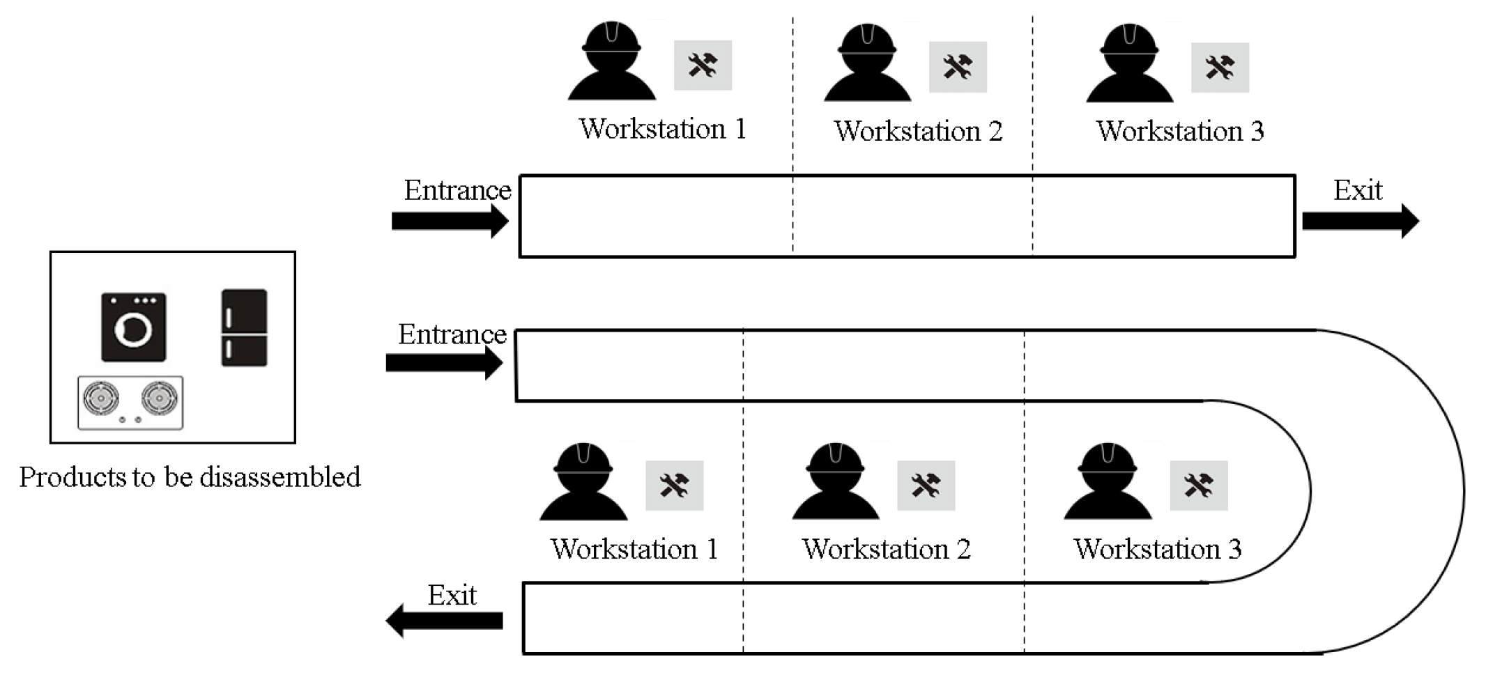
Referring to the HDLBP illustration in Figure 4, where the product needs to be disassembled, there are two workstations on each line, and the specific meaning of the action selection code is shown in Table 4. There are two steps for each disassembly product. The first step is to select the disassembly line of the product, and the second step is to assign the disassembly task to the workstation. In order to distinguish the inlet and outlet sides of the UDL workstation, two workstations have four options. When a product is allocated to a LDL, the task assignment to workstations is contingent upon the output values of the task selection, where values 0 or 1 assign to workstation 1, whereas values 2 or 3 assign to workstation 2. In the UDL, an output value of 0 directs task assignment to the entry side of workstation 1; a value of 1 corresponds to assignment at the entry side of workstation 2; a value of 2 leads to assignment at the exit side of workstation 2; and a value of 3 triggers assignment at the outlet side of workstation 1. Specific values represent unique disassembly selection operations, with the target value set according to the chosen operation.
As shown in Figure 4, the agent may randomly choose the action code [0, 1, 2, 2] for product 1; this indicates that product 1 is slated for disassembly on the LDL, with task 1 being assigned to workstation 1, and tasks 2 and 3 being allocated to workstation 2.
Algorithm 1 shows the pseudocode of action for disassembly tasks. It takes as inputs the disassembly parameters, the action space, and the observation space. The outputs of the algorithm are obj1 and obj2. The algorithm operates in an iterative manner, looping over each product. For each product, it selects a disassembly line from the action space based on the assigned action for that particular product, stored in the variable l i n e . If l i n e is equal to 0, it means that the disassembly will take place on a linear workstation. In this case, the algorithm enters a nested loop, iterating over each task associated with the disassembly. Within this loop, it retrieves the assigned action for the current product and task, stored in the variable l i n e a r _ w o r k s t a t i o n , and applies Algorithm 2.
Lastly, the algorithm calculates obj1 and obj2. On the other hand, if l i n e is not equal to 0, it implies that the disassembly will occur on a U-shaped workstation. The algorithm follows a similar pattern as above, but this time the assigned action for the current product and task is retrieved and stored in the variable U s h a p e d _ w o r k s t a t i o n before applying Algorithm 2. Finally, obj1 and obj2 are calculated. After processing all products, the algorithm returns obj1 and obj2 as the final output. In summary, the algorithm determines the disassembly line for each product based on the assigned actions, performs the corresponding disassembly tasks using the specified workstations (either linear or U-shaped), and calculates obj1 and obj2 as the results of these operations.
Algorithm 2 described in the pseudocode is called “action correction and decoding”. The inputs to the algorithm are two arrays, a linear workstation denoted by L W and a U-shaped workstation denoted by U W , as well as a line parameter indicating which type of workstation is being used. The outputs of the algorithm are the updated version of the two workstations L W and U W . The algorithm first sorts the values of the workstations in ascending order and then checks the value of the line parameter. If the line parameter equals 0, each element in the workstation arrays is updated based on its original value. Specifically, if the value is either 0 or 3, it is changed to 1; if the value is either 1 or 4, it is changed to 2; otherwise, it is changed to 3.
On the other hand, if the line parameter equals 1, each element in the workstation arrays is also updated based on its original value, but following a different set of rules. Specifically, if the value is either 0 or 5, it is changed to 1; if the value is either 1 or 4, it is changed to 2; otherwise, it is changed to 3. In summary, the algorithm provides a method for correcting and decoding the actions taken at two different types of workstations, based on their original values and the type of the production line being used. Handling incorrect actions can be achieved by providing negative feedback rewards to reduce the probability of the agent selecting incorrect actions. However, at the same time, training efficiency would significantly decrease, necessitating an increase in the number of training iterations to obtain satisfactory results. In contrast, correcting incorrect actions can accelerate training speed and enhance the agent’s exploration capabilities. It can also lead to better quality solutions within the same number of training iterations compared to negative feedback reward methods.
(3) Reward Function
In the definition of reward, we evaluate the reward that the agent can obtain in this state according to the quality of the multi-objective solution. Firstly, a memory pool is established to store the multi-objective solution of the training process, and the experience pool is empty in the initial state. The solution obtained by training during the first round can be successfully stored in the memory pool and a positive feedback reward can be obtained. Whether the solution of each subsequent training can enter the memory pool is determined according to the dominance relationship. Assuming that the new solution is o b j 1 , o b j 2 , the minimum value and maximum value of target 1 in the memory pool is x 1 , x 2 , and the minimum value maximum value of target 2 is y 1 , y 2 . We set the reward coefficient α 1 and α 2 . The specific circumstances of the reward are divided into the following three.
For the repeated solution, we use the reward coefficient α 1 and α 2 to guide the exploration direction of the agent. In the initial state, both α 1 and α 2 values are 1. When the repeated solution belongs to the first kind, reducing the value of α 1 increases the value of α 2 , and guides the agent to explore on the same Pareto front. When the repeated solution belongs to the second kind, increasing the value of α 1 and decreasing the value of α 2 will lead the agent to explore the better solution.
The pseudocode in Algorithm 3 outlines a framework for the Non-Dominated Sort in A2C. The algorithm takes two input objectives, namely obj1 and obj2, and produces a single output reward. The algorithm begins by initializing the parameters, including the memory pool D and the weighting factors α 1 and α 2 , both set to 1. For each iteration, the algorithm proceeds to perform environment steps. If the memory pool D is not empty, the algorithm identifies the minimum and maximum values of “target1” as x 1 and x 2 , respectively, and the minimum and maximum values of “target2” as y 1 and y 2 , respectively. Next, the algorithm checks if obj1 is greater than x 2 and obj2 is less than y 1 . If this condition is satisfied, it further checks whether the solution is repeated. If the solution is repeated, the weighting factors are updated ( α 1 = 0.5 , α 2 = 2 ), and the reward is calculated as 100 α 1 . Otherwise, the reward is calculated as 100 α 1 , and the memory pool D is updated. If the previous condition is not satisfied, the algorithm checks if obj1 is less than x 1 or “obj2” is greater than y 2 . Again, if the solution is repeated, the weighting factors are updated ( α 1 = 2 , α 2 = 0.5 ), and the reward is calculated as 100 α 2 . Otherwise, the reward is calculated as 100 α 2 , and the memory pool D is updated.
The pseudocode in Algorithm 4 uses the environment E n v and the number of episodes N as input parameters. The algorithm first initializes the policy network π and the value network V, as well as the optimizers for the policy network and the value network. Then, for each episode e p i s o d e , the algorithm resets the environment and initializes the current state s, clearing the episode buffer. In each episode, the algorithm selects an action a from the current state s using the policy network π , executes the action a, uses Algorithms 1 and 3 to calculate reward r, observes the reward r and the next state s , and stores the state transition ( s , a , r , s ) in the episode buffer. Then, the state s is updated to s . When the episode is finished, the algorithm calculates the discounted rewards R t for each time step t in the episode buffer, as well as the advantages A t = R t V ( s t ) for each time step t. Next, the algorithm uses gradient ascent to update the parameters θ π of the policy network π based on the expected cumulative rewards. Then, the algorithm uses the mean squared error loss function to update the parameters θ V of the value network V based on the difference between the predicted and actual rewards. Finally, the algorithm repeats this process until all episodes are completed and returns the learned policy network π as output.
Algorithm 4: MO-A2C.
Information 15 00168 i004

5. Experiments

In order to verify the superiority of the MO-A2C algorithm, we compare it with the SAC, DDPG, and NSGAII algorithms. We utilize the stable-baselines3 framework [28] to implement and train the reinforcement learning algorithm. The experiment employs the default parameter configurations provided by the framework. The initial population of the NSGAII algorithm is set to 50, and the number of iterations is 200. Evaluation indicators are spread [5], epsilon [29], and inverted generational distance plus (IGD+) [30]. The meaning of each metric is given as follows.
(1) Spread: It is used to measure the distribution range of the Pareto frontier. The value range of Spread is 0 to 1. When the value of Spread is closer to 1, the diversity and distribution uniformity of the solution set are better. When the value of Spread is closer to 0, the diversity and distribution uniformity of the solution set are worse.
(2) Epsilon Metric: It is used to measure the distance between the approximate to the Pareto frontier and the real Pareto frontier. The smaller Epsilon Metric value indicates that the approximate Pareto front is closer to the real Pareto front, indicating that the algorithm is better in the coverage of the solution set. When the value of Epsilon Metric is equal to 0, it means that the approximate Pareto front is completely coincident with the real Pareto front wherein the optimal solution is completely found.
(3) IGD+ Metric: It quantifies the dissimilarity between an approximate Pareto front and the true Pareto front, thereby providing insights into the quality of the obtained solution set. A smaller IGD+ value denotes a higher quality approximation. In order to mitigate the possibility of obtaining experimental results by chance, this study employs the t-test [31].

5.1. Disassembly Instances

The products selected for disassembly are televisions, cellphones [32], and Tesla batteries [33]. Televisions and cellphones are small-scale disassembly items, while Tesla batteries are large-scale. We assume that the maximum number of skills required to perform the task of disassembly of a product is 5, as indicated in Table 5. An interval random distribution is used to develop workers’ disassembly skills and task profit parameters. Every disassembly instance comprises a heterogeneous assortment of products. The details of each instance are presented in Table 6.

5.2. Analysis of Experimental Results

The model for each case undergoes training for 1000 timesteps. Figure 6 shows the Pareto front obtained by the algorithms for solving different cases. Table 7 shows the performance indicators of different algorithms. The sign ’+’ indicates that the SAC is significantly superior to the other two algorithms, ’∼ ’ indicates that the SAC is approximately equal to the other two algorithms, and ’−’ indicates that the SAC is significantly inferior to the other two algorithms.
In Case 1, the resultant Pareto front comprises solutions generated by four distinct algorithms. Considering the dispersion level among the objectives within the solution space, it is evident that the NSGAII algorithm possesses certain advantages in this regard. Moreover, when evaluating the dissimilarity between the approximated Pareto front and the actual Pareto front, both the A2C and SAC algorithms have exhibited commendable performance indicators. Based on the analysis of Figure 6a alongside these performance metrics, it can be concluded that the A2C algorithm outperforms other methods in effectively addressing Case 1.
In Case 2, it is observed that the DDPG algorithm exhibits a superior degree of dispersion among the objectives. However, when considering additional performance indicators such as the Epsilon and IGD+ metrics, the SAC algorithm emerges as the frontrunner among the various algorithms evaluated. Consequently, in terms of overall performance, the SAC algorithm proves to be more effective in tackling and resolving Case 2.
With regards to Case 3 and Case 4, it is evident that both the A2C and NSGAII algorithms exhibit several advantages vis-à-vis performance indicators. However, when considering solution quality, the NSGAII algorithm demonstrates comparable performance levels to that of other evaluated algorithms.
In Case 5, it is observed that the DDPG algorithm exhibits enhanced performance in terms of dispersion, whereas the NSGAII algorithm demonstrates superior performance in capturing the dissimilarity between the approximated Pareto frontier and the actual Pareto frontier. By analyzing Figure 6e, it can be deduced that both the A2C and NSGAII algorithms yield comparable solution quality.
In Case 6, it is noted that the DDPG algorithm exhibits superior performance in terms of dispersion. Conversely, the A2C algorithm demonstrates optimal performance in capturing the dissimilarity between the approximated Pareto frontier and the actual Pareto frontier. Furthermore, based on the analysis of Figure 6f, it is concluded that the A2C algorithm surpasses other algorithms in terms of overall performance in Case 6.
In solving the HDLBP, according to the above experimental results, the MO-A2C has certain advantages in solving this problem. Although the NSGAII algorithm has some advantages in some cases, it relies more on the crossover operator and mutation operator. The design of the crossover operator and mutation operator requires much time to try. With the complexity of the problem scale, the design of the operator is becoming more and more difficult. Secondly, in the initial population and iteration settings, we set 20, 30, 40 populations to iterate 200 times, respectively, and there is only one final output solution. When the population size is increased to 50, two solutions are formed after 200 iterations. The running time of the algorithm is also prolonged. On the whole, the algorithm running time of reinforcement learning in solving HDLBP is better than that of the NSGAII algorithm, whether in the solution scheme or in the quality of the solution.
In the previous work, we use RL to solve the single-objective HDLBP, and the experimental results show that the SAC algorithm performs best. For dealing with HDLBP, A2C performs better than DDPG and SAC, mainly because A2C usually uses deterministic strategy or greedy strategy with noise to sample actions, while SAC uses Gaussian distribution to add a standard deviation to the mean of actions to sample actions, so as to increase the exploratory of strategies. DDPG uses a deterministic strategy network to select actions and output the mean of continuous actions. Since the optimization goal is two goals, the greedy strategy can often explore more types of solutions in a short period of training. Secondly, the problem is a discrete problem. Although we have made some improvements to the SAC and DDPG algorithms in action selection, it may not be perfectly adapted to deal with discrete multi-objective problems. In particular, the performance of DDPG can be sensitive to the choice of hyperparameters and the possible noise process used for exploration.

6. Conclusions

In this paper, the multi-objective balancing problem of a hybrid disassembly line with multi-skilled disassembly workers is studied for the first time. The objective of the HDLBP is to maximize revenue from disassembly and minimize carbon emissions. To effectively address this challenge, both discrete and continuous action spaces are formulated, and an interaction environment is established between RL agent and the hybrid disassembly line. The reward function is optimized in RL algorithm, and the degree of excellence of the solution is used as an evaluation index. The reward coefficient is set to change the agent’s exploration on the Pareto front to obtain better solutions. Simulation experiments are carried out to verify the correctness of the model and the RL algorithm’s performance. In some of the experimental cases in this paper, the solutions produced by the multi-objective Advantage Actor-Critic algorithm show some advantages over other popular algorithms such as the Deep Deterministic Policy Gradient Algorithm, the Soft Actor-Critic Algorithm, and the Non-Dominated Sorting Genetic Algorithm II.
The current limitations of MO-A2C are mainly in the convergence problem and the high latitude problem. (1) Convergence problem may be faced when searching for Pareto frontiers, especially when there are conflicts or complex nonlinear relationships between the objectives. (2) MO-A2C may face exploration and generalization difficulties in high-dimensional states and action spaces, which leads to the difficulty of generalization of the learned strategies to complex environments. In future research, we plan to combine deep reinforcement learning with evolutionary algorithms to better handle multi-objective optimization problems [34]. Evolutionary algorithms can provide a more global search strategy and accelerate the convergence of reinforcement learning algorithms. (3) We will use the improved MO-A2C to explore the performance of solving more multi-objective problems, such as three objectives, four objectives, or more. There is also the extension of MO-A2C to multi-intelligent body systems to deal with more complex collaborative and competitive scenarios and to enhance the exploration capabilities of intelligent bodies.

Author Contributions

Conceptualization, J.W. and X.G.; methodology, S.Q.; validation, G.X.; writing—original draft preparation, G.X.; writing—review and editing, J.W.; visualization, H.H.; supervision, J.W. All authors have read and agreed to the published version of the manuscript.

Funding

This work is supported in part by NSFC under Grant 61903229, in part by Liaoning Revitalization Talents Program under Grant XLYC1907166, in part by the Natural Science Foundation of Shandong Province under Grant ZR2019BF004, and in part by Archival Science and Technology Project of Liaoning Province under Grant 2021-B-004.

Institutional Review Board Statement

Not applicable.

Informed Consent Statement

Not applicable.

Data Availability Statement

The data presented in this study are available on request from the corresponding author.

Conflicts of Interest

The authors declare no conflicts of interest.

Nomenclature

LDLLinear disassembly line
UDLU-shaped disassembly line
D = [ d j k p ] describes the relationship between any two tasks
B = [ b j n p ] the relationship between tasks and skills
A = [ a w n l ] describe the relationship between worker and skills
P Set of EOL products, P = { 1 , 2 , , p }
J p Number of tasks in product p
L Set of all disassembly lines
W 1 Set of workstations in the LDL, W 1 =   1 , 2 , , W 1
W 2 Set of workstations in the UDL, W 2 = 1 , 2 , , W 2 .
S Set of the two sides of UDL workstation, S = { 1 , 2 }
N Set of all needed skills, N = { 1 , 2 , , N }
v p j The benefit of the j-th disassembly task of the p-th product
t p j The time needed to execute the j-th task of the p-th product
c p j The time unit cost of executing the j-th task of the p-th product
c l The time unit cost of executing the l-th disassembly line
c w The time unit cost of executing the w-th workstation
α l w n The worker on workstation w-th on the l-th disassembly line has the n-th skill
β p j n The j-th task of the p-th product requires the use of n-th skill
T l Cycle time of disassembly line l
P W i l Load power of the i-th workstation on the l-th disassembly line
P D l Transmission power of disassembly line l
z p l Decision variable, 1, product p assigned to disassembly line l, 0, otherwise
x p j w 1 Decision variable, 1, task j of product p is assigned to LDL workstation w ( w W 1 ) , 0, otherwise
x p j w s 2 Decision variable, 1, task j of product p is assigned to the s side of UDL workstation w ( w W 2 ) , 0, otherwise
y l Decision variable, 1, disassembly line l is activated, 0, otherwise
u l w Decision variable, 1, workstation w of disassembly line l is activated, 0, otherwise
x i l w n Decision variable, 1, if a worker on workstation w of the disassembly line l uses skill n ( n N ) , 0, otherwise
DLBPDisassembly Line Problem
HDLBPHybrid Disassembly Line Balancing Problem
A2CAdvantage Actor-Critic
MO-A2CMulti-Objective Advantage Actor-Critic
DDPGDeep Deterministic Policy Gradient
SACSoft Actor-Critic
NSGAIINon-Dominated Sorting Genetic Algorithm II
Sset of all possible states in the environment
Aset of all actions that the agent can take
Pthe probability of state transition to s after taking action a in state s.
Rthe reward obtained when the state s takes action a and moves to the state s
γ discount factor

References

  1. Hezer, S.; Kara, Y. A network-based shortest route model for parallel disassembly line balancing problem. Int. J. Prod. Res. 2015, 53, 1849–1865. [Google Scholar] [CrossRef]
  2. Qin, S.; Zhang, S.; Wang, J.; Liu, S.; Guo, X.; Qi, L. Multi-objective multi-verse optimizer for multi-robotic u-shaped disassembly line balancing problems. IEEE Trans. Artif. Intell. 2023, 5, 882–894. [Google Scholar] [CrossRef]
  3. Liang, J.; Guo, S.; Du, B.; Li, Y.; Guo, J.; Yang, Z.; Pang, S. Minimizing energy consumption in multi-objective two-sided disassembly line balancing problem with complex execution constraints using dual-individual simulated annealing algorithm. J. Clean. Prod. 2021, 284, 125418. [Google Scholar] [CrossRef]
  4. Zhu, L.; Zhang, Z.; Guan, C. Multi-objective partial parallel disassembly line balancing problem using hybrid group neighborhood search algorithm. J. Manuf. Syst. 2020, 56, 252–269. [Google Scholar] [CrossRef]
  5. Wu, J.; Azarm, S. Metrics for quality assessment of a multiobjective design optimization solution set. J. Mech. Des. 2001, 123, 18–25. [Google Scholar] [CrossRef]
  6. Li, S.; Wu, Y.; Cui, X.; Dong, H.; Fang, F.; Russell, S. Robust multi-agent reinforcement learning via minimax deep deterministic policy gradient. In Proceedings of the AAAI Conference on Artificial Intelligence, Honolulu, HI, USA, 27 January–1 February 2019; Volume 33, pp. 4213–4220. [Google Scholar]
  7. Haarnoja, T.; Zhou, A.; Abbeel, P.; Levine, S. Soft actor-critic: Off-policy maximum entropy deep reinforcement learning with a stochastic actor. In Proceedings of the International Conference on Machine Learning. PMLR, Stockholm, Sweden, 10–15 July 2018; pp. 1861–1870. [Google Scholar]
  8. Deb, K.; Agrawal, S.; Pratap, A.; Meyarivan, T. A fast elitist non-dominated sorting genetic algorithm for multi-objective optimization: NSGA-II. In Proceedings of the Parallel Problem Solving from Nature PPSN VI: 6th International Conference, Paris, France, 18–20 September 2000; Proceedings 6. Springer: Berlin/Heidelberg, Germany, 2000; pp. 849–858. [Google Scholar]
  9. Wang, J.; Xi, G.; Guo, X.; Liu, S.; Qin, S.; Han, H. Reinforcement learning for Hybrid Disassembly Line Balancing Problems. Neurocomputing 2024, 569, 127145. [Google Scholar] [CrossRef]
  10. Wang, K.; Li, X.; Gao, L. Modeling and optimization of multi-objective partial disassembly line balancing problem considering hazard and profit. J. Clean. Prod. 2019, 211, 115–133. [Google Scholar] [CrossRef]
  11. Li, Z.; Janardhanan, M.N. Modelling and solving profit-oriented U-shaped partial disassembly line balancing problem. Expert Syst. Appl. 2021, 183, 115431. [Google Scholar] [CrossRef]
  12. Zhu, L.; Zhang, Z.; Wang, Y. A Pareto firefly algorithm for multi-objective disassembly line balancing problems with hazard evaluation. Int. J. Prod. Res. 2018, 56, 7354–7374. [Google Scholar] [CrossRef]
  13. Zhang, L.; Zhao, X.; Ke, Q.; Dong, W.; Zhong, Y. Disassembly line balancing optimization method for high efficiency and low carbon emission. Int. J. Precis. Eng. Manuf.-Green Technol. 2021, 8, 233–247. [Google Scholar] [CrossRef]
  14. Yang, Y.; Yuan, G.; Zhuang, Q.; Tian, G. Multi-objective low-carbon disassembly line balancing for agricultural machinery using MDFOA and fuzzy AHP. J. Clean. Prod. 2019, 233, 1465–1474. [Google Scholar] [CrossRef]
  15. McGovern, S.M.; Gupta, S.M. A balancing method and genetic algorithm for disassembly line balancing. Eur. J. Oper. Res. 2007, 179, 692–708. [Google Scholar] [CrossRef]
  16. Qiu, Y.; Wang, L.; Xu, X.; Fang, X.; Pardalos, P.M. A variable neighborhood search heuristic algorithm for production routing problems. Appl. Soft Comput. 2018, 66, 311–318. [Google Scholar] [CrossRef]
  17. Mazyavkina, N.; Sviridov, S.; Ivanov, S.; Burnaev, E. Reinforcement learning for combinatorial optimization: A survey. Comput. Oper. Res. 2021, 134, 105400. [Google Scholar] [CrossRef]
  18. Zhao, X.; Li, C.; Tang, Y.; Cui, J. Reinforcement Learning-Based Selective Disassembly Sequence Planning for the End-of-Life Products With Structure Uncertainty. IEEE Robot. Autom. Lett. 2021, 6, 7807–7814. [Google Scholar] [CrossRef]
  19. Guo, X.; Bi, Z.; Wang, J.; Qin, S.; Liu, S.; Qi, L. Reinforcement learning for disassembly system optimization problems: A survey. Int. J. Netw. Dyn. Intell. 2023, 2, 1–14. [Google Scholar] [CrossRef]
  20. Shuvo, S.S.; Symum, H.; Ahmed, M.R.; Yilmaz, Y.; Zayas-Castro, J.L. Multi-Objective Reinforcement Learning Based Healthcare Expansion Planning Considering Pandemic Events. IEEE J. Biomed. Health Inform. 2022, 27, 2760–2770. [Google Scholar] [CrossRef]
  21. Amidzadeh, M. A Scale-Independent Multi-Objective Reinforcement Learning with Convergence Analysis. arXiv 2023, arXiv:2302.04179. [Google Scholar]
  22. Zheng, H.; Zhang, Z.; Zeng, Y. Multi-objective U-shaped demolition line equilibrium problem with uncertain worker physical exertion. Comput.-Integr. Manuf. Syst. 2023, 29, 392–403. [Google Scholar]
  23. Guo, X.; Wei, T.; Wang, J.; Liu, S.; Qin, S.; Qi, L. Multiobjective U-shaped disassembly line balancing problem considering human fatigue index and an efficient solution. IEEE Trans. Comput. Soc. Syst. 2022, 10, 2061–2073. [Google Scholar] [CrossRef]
  24. Ming, H.; Liu, Q.; Pham, D.T. Multi-robotic disassembly line balancing with uncertain processing time. Procedia CIRP 2019, 83, 71–76. [Google Scholar] [CrossRef]
  25. Xu, Z.; Han, Y. Two sided disassembly line balancing problem with rest time of works: A constraint programming model and an improved NSGA II algorithm. Expert Syst. Appl. 2024, 239, 122323. [Google Scholar] [CrossRef]
  26. Xu, S.; Guo, X.; Liu, S.; Qi, L.; Qin, S.; Zhao, Z.; Tang, Y. Multi-objective Optimizer with Collaborative Resource Allocation Strategy for U-shaped Stochastic Disassembly Line Balancing Problem. In Proceedings of the 2021 IEEE International Conference on Systems, Man, and Cybernetics (SMC), IEEE, Melbourne, Australia, 17–20 October 2021; pp. 2316–2321. [Google Scholar]
  27. Zheng, Y.; Li, X.; Xu, L. Balance control for the first-order inverted pendulum based on the advantage actor-critic algorithm. Int. J. Control. Autom. Syst. 2020, 18, 3093–3100. [Google Scholar] [CrossRef]
  28. Raffin, A.; Hill, A.; Gleave, A.; Kanervisto, A.; Ernestus, M.; Dormann, N. Stable-Baselines3: Reliable Reinforcement Learning Implementations. J. Mach. Learn. Res. 2021, 22, 1–8. [Google Scholar]
  29. Qi, L.; Zhou, M.; Luan, W. A dynamic road incident information delivery strategy to reduce urban traffic congestion. IEEE/CAA J. Autom. Sin. 2018, 5, 934–945. [Google Scholar] [CrossRef]
  30. Ishibuchi, H.; Masuda, H.; Tanigaki, Y.; Nojima, Y. Modified distance calculation in generational distance and inverted generational distance. In Proceedings of the Evolutionary Multi-Criterion Optimization: 8th International Conference, EMO 2015, Guimarães, Portugal, 29 March–1 April 2015; Proceedings, Part II 8. Springer: Berlin/Heidelberg, Germany, 2015; pp. 110–125. [Google Scholar]
  31. Gosset, W.S. The probable error of a mean. Biometrika 1908, 6, 1–25. [Google Scholar]
  32. Igarashi, K.; Yamada, T.; Inoue, M. 2-stage optimal design and analysis for disassembly system with environmental and economic parts selection using the recyclability evaluation method. Ind. Eng. Manag. Syst. 2014, 13, 52–66. [Google Scholar] [CrossRef]
  33. Wu, T.; Zhang, Z.; Yin, T.; Zhang, Y. Multi-objective optimisation for cell-level disassembly of waste power battery modules in human-machine hybrid mode. Waste Manag. 2022, 144, 513–526. [Google Scholar] [CrossRef]
  34. Tian, Y.; Li, X.; Ma, H.; Zhang, X.; Tan, K.C.; Jin, Y. Deep reinforcement learning based adaptive operator selection for evolutionary multi-objective optimization. IEEE Trans. Emerg. Top. Comput. Intell. 2022, 7, 1051–1064. [Google Scholar] [CrossRef]
Figure 1. An example of a hybrid disassembly line layout.
Information 15 00168 g001
Figure 2. Computer components and precedence graph of disassembly tasks. (a) Components of a computer; (b) Precedence graph of the computer disassembly tasks.
Information 15 00168 g002
Figure 3. The MO-A2C decision framework for solving HDLBP.
Information 15 00168 g003
Figure 4. The action design for an HDLBP instance.
Information 15 00168 g004
Figure 5. Update of reward.
Information 15 00168 g005
Figure 6. Pareto front of the different instances. (a) Test instance 1; (b) Test instance 2; (c) Test instance 3; (d) Test instance 4; (e) Test instance 5; (f) Test instance 6.
Information 15 00168 g006
Table 1. Related literature on the mutiobjective disassembly line balancing problem.
LiteraturesDisassembly LevelNumber of ProductsLine LayoutOptimization ObjectivesSolving Method
Zhu, L. [12]CompleteSingleStraightMultiple (Pareto)Pareto firefly algorithm
Zhang, L. [13]CompleteSingleStraightMultiple (Pareto)Improved genetic algorithm
Yang, Y. [14]CompleteSingle-Multiple (Pareto)Improved fruit fly optimization algorithm
Zhao, X. [18]PartialSingle-Multiple (Pareto)Improved Deep q Network algorithm
Our studyCompleteMixed productStraight and U-shaped (Hybrid)Multiple (Pareto)MO-A2C
Table 2. Disassembly tasks of a computer.
IndexDisassembly Task NameIndexDisassembly Task NameIndexDisassembly Task Name
1Front bezel11Backshell screws21Drive plate screws
2Base screws 112Backshell22Driver board
3Foundation13Backshell retaining tab screws23Protective case for power plate
4Chassis border14Backshell fixing piece24Left rear shell mounting plate
5Base plate15Keypad screws25Right rear shell mounting plate
6Base support plate16Keypad26Screensaver
7Base screws 217Power board wiring27Logic board protection board
8Chassis fixing piece18Power board screws28Circuit board 1
9Left adjuster19Power supply board29Circuit board 2
10Right adjuster20Driver board30Screen
Table 3. Relationship between workers and skills.
Disassembly Line TypeWorkerSkill
12
Linear101
200
310
U-shaped111
200
311
Table 4. Action selection code.
Disassembly Line SelectionWorkstation Selection
0LDL0 or 1W1
2 or 3W2
1UDL0inlet side of W1
1inlet side of W2
2outlet side of W1
3outlet side of W2
Table 5. Products for disassembly test.
ProductNumber of TasksNumber of Required Skills
TV125
Cellphone125
Tesla battery375
Table 6. Test instances.
Instance IDNumber of ProductsNumber of Tasks
TVCellphoneTesla Battery
111024
212036
301149
411161
5122110
6223159
Table 7. Comparison of four algorithms.
Case IDAlgorithmSpreadEpsilonIGD+
Meant-TestMeant-TestMeant-Test
1MO-A2C0.68326/0.16570/0.07493/
SAC0.52565+0.19268+0.05041
DDPG0.29654+0.59322+0.30046+
NSGAII0.749230.46243+0.25388+
2MO-A2C0.72013/0.88462/0.35328/
SAC0.60091+0.240380.10058
DDPG0.813300.839290.40801+
NSGAII0.61292+1.00000+0.31346
3MO-A2C0.84774/0.72228/0.50514/
SAC0.43133+0.87591+0.52413+
DDPG0.81568+1.03901+1.07308+
NSGAII0.51018+0.175180.05839
4MO-A2C0.97417/0.72228/0.35058/
SAC0.88987+0.97620+0.34989
DDPG0.81841+0.97268+0.35387
NSGAII0.94202+0.99873+0.32324
5MO-A2C0.48166/0.50035/0.16293/
SAC0.707751.70000+1.42880+
DDPG0.968832.60000+2.18753+
NSGAII0.29909+0.160000.06285
6MO-A2C0.69450/0.05172/0.01034/
SAC0.696431.31071+0.86312+
DDPG0.935452.17241+2.38087+
NSGAII0.828310.57321+0.25021+
Disclaimer/Publisher’s Note: The statements, opinions and data contained in all publications are solely those of the individual author(s) and contributor(s) and not of MDPI and/or the editor(s). MDPI and/or the editor(s) disclaim responsibility for any injury to people or property resulting from any ideas, methods, instructions or products referred to in the content.

