A New Time Series Dataset for Cyber-Threat Correlation, Regression and Neural-Network-Based Forecasting

Abstract

In the face of escalating cyber threats that have contributed significantly to global economic losses, this study presents a comprehensive dataset capturing the multifaceted nature of cyber-attacks across 225 countries over a 14-month period from October 2022 to December 2023. The dataset, comprising 77,623 rows and 18 fields, provides a detailed chronology of cyber-attacks, categorized into eight critical dimensions: spam, ransomware, local infection, exploit, malicious mail, network attack, on-demand scan, and web threat. The dataset also includes ranking data, offering a comparative view of countries’ susceptibility to different cyber threats. The results reveal significant variations in the frequency and intensity of cyber-attacks across different countries and attack types. The data were meticulously compiled using modern AI-based data acquisition techniques, ensuring a high degree of accuracy and comprehensiveness. Correlation tests against the eight types of cyber-attacks resulted in the determination that on-demand scan and local infection are highly correlated, with a correlation coefficient of 0.93. Lastly, neural-network-based forecasting of these highly correlated factors (i.e., on-demand scan and local infection) reveals a similar pattern of prediction, with an MSE and an MAPE of 1.616 and 80.13, respectively. The study’s conclusions provide critical insights into the global landscape of cyber threats, highlighting the urgent need for robust cybersecurity measures.

1. Introduction

In the contemporary digital landscape, cyber-attacks have emerged as formidable threats, inflicting substantial economic and security damages globally. Recent estimates suggest that these attacks have contributed to an alarming USD 3.5 trillion in economic losses, underscoring the urgency for comprehensive research in this domain [1,2]. Other than the detrimental economic impact, it has become increasingly evident that cyber-attacks manifest profound influences within both the psychological and behavioral strata, precipitating far-reaching ramifications at the societal echelon [3]. Addressing this critical need, our research team has compiled an extensive dataset, encompassing a period from 11 October 2022 to December 2023, marking a significant stride in understanding and mitigating the impacts of cyber threats.

This novel dataset, unprecedented in its scope and detail, covers 399 dates over 14 months, meticulously gathered from open-source daily statistics (e.g., Kaspersky [4]). It encapsulates data on eight critical dimensions of cyber-attacks: spam [5], ransomware [6], local infection [7], exploit [8], malicious mail [9], network attack [10], on-demand scan [11], and web threat [12]. The dataset’s global reach, spanning 225 countries, provides a comprehensive view of the cyber-threat landscape, making it an invaluable resource for longitudinal studies in this field. The dataset offers both percentage-wise attack statistics and world-ranking-wise attack statistics, offering researchers a multifaceted view of the cyber-threat landscape. Though some of our recent projects have already utilized a smaller subset of this dataset, demonstrating its versatility and applicability across various domains [13,14,15,16], the full dataset had yet to be publicly released (as shown in

Table 1. Summary of the contributions of this study.

Reference	Start Date	End Date	Day	Public Release with Data Descriptors	Correlation Analysis	Regression Analysis	Neural-Network-Based Forecasting
[13]	11 October 2022	31 October 2022	21	No	No	No	No
[16]	11 October 2022	25 December 2022	76	No	No	No	No
[15]	11 October 2022	6 April 2023	178	No	No	No	No
[14]	11 October 2022	12 July 2023	275	No	No	No	No
This	11 October 2022	11 December 2023	427	Yes	Yes	Yes	Yes

). The public release and description of this dataset offers numerous benefits. It not only fosters transparency and collaboration among researchers but also accelerates the development of effective countermeasures against cyber threats. By providing a rich source of empirical data, it enables the scientific community to conduct more nuanced and comprehensive analyses (as well as predictions), ultimately contributing to the enhancement of global cyber resilience. The data acquisition process employed modern AI-based techniques, ensuring high accuracy and reliability. These techniques included advanced data manipulation and integration methods, tailored to capture the nuanced dynamics of cyber-attacks.

In the last six years there have studies that have focused on the regression [17,18,19], correlation [20,21], and prediction [22,23,24,25,26,27,28,29] of cyber-attacks in order to boost cyber preparedness. However, because of the lack of a robust cyber-attack dataset, these existing studies faced limitations in terms of their prediction accuracy. After generating the novel and robust dataset in this study, several attempts at statistical modelling (e.g., correlation, regression etc.) were performed, along with predictions related to cyber threats against randomly selected countries like Australia, New Zealand, Qatar, Saudi Arabia, and UAE. A thorough performance evaluation revealed a higher accuracy in predicting cyber threats, in comparison with existing studies [22,23,24,25,26,27,28,29].

The core contributions of this study can be succinctly summarized as follows:

• Innovative methodology: We developed an automated methodology for the systematic collection of global cyber-attack data, offering a novel and efficient approach to dataset creation.
• Comprehensive dataset: We generated a comprehensive dataset spanning 225 countries over a 14-month period, comprising 77,623 rows and 18 fields, capturing the multifaceted nature of cyber-attacks across diverse dimensions (publicly available at https://github.com/DrSufi/CyberData, accessed on 14 February 2024).
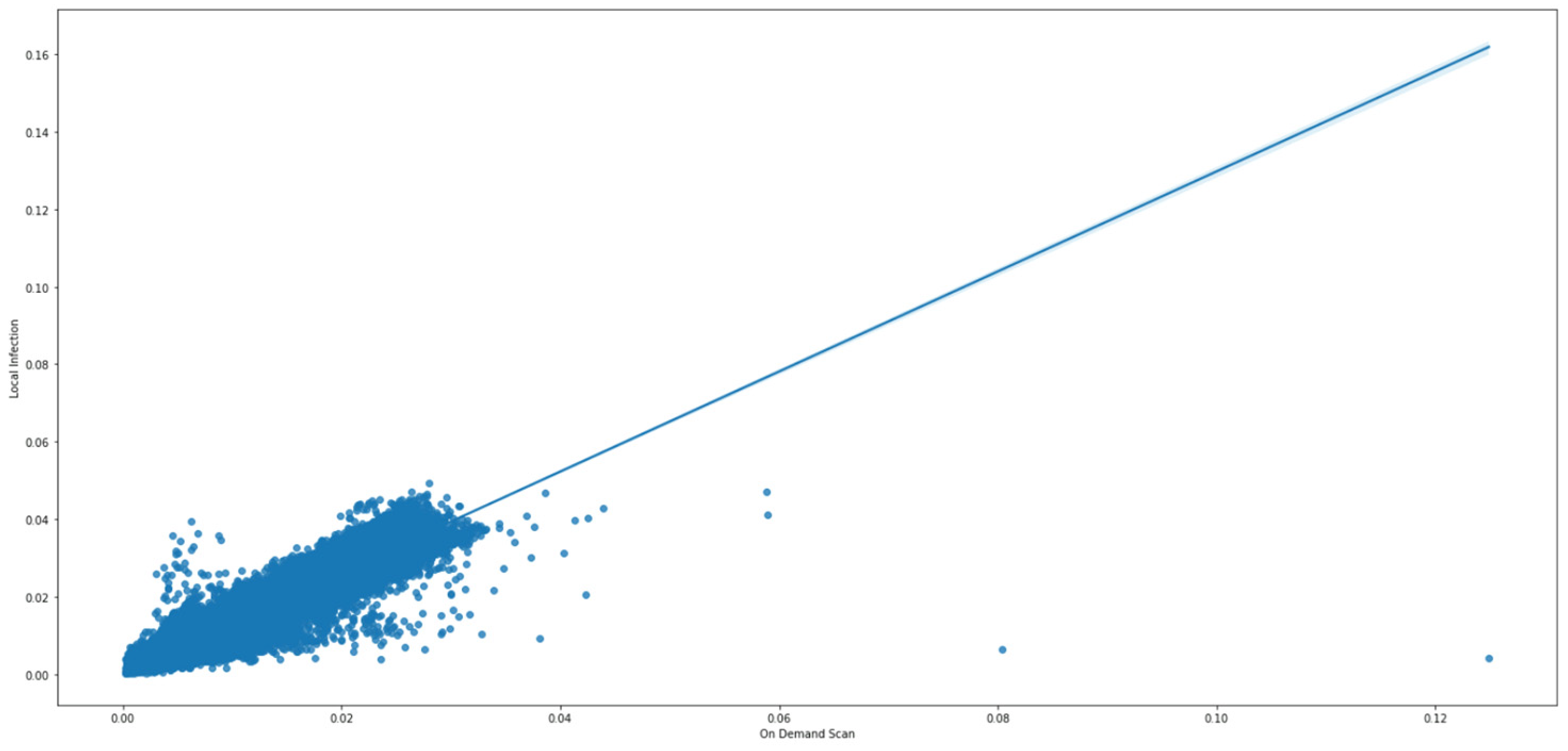
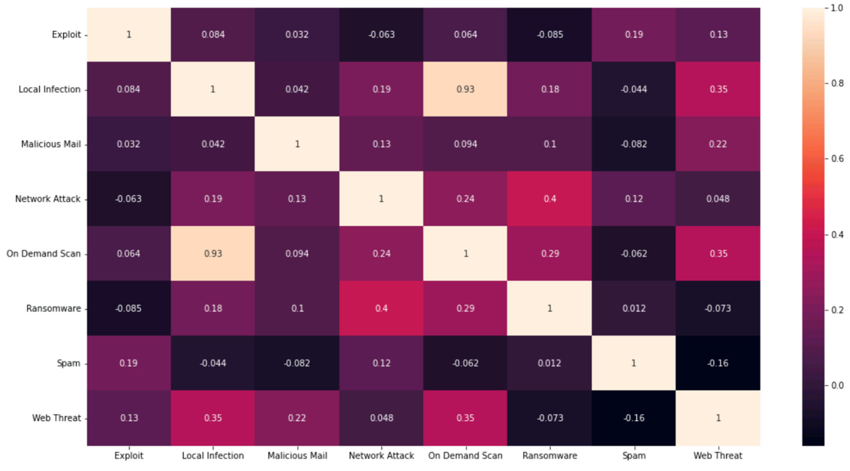
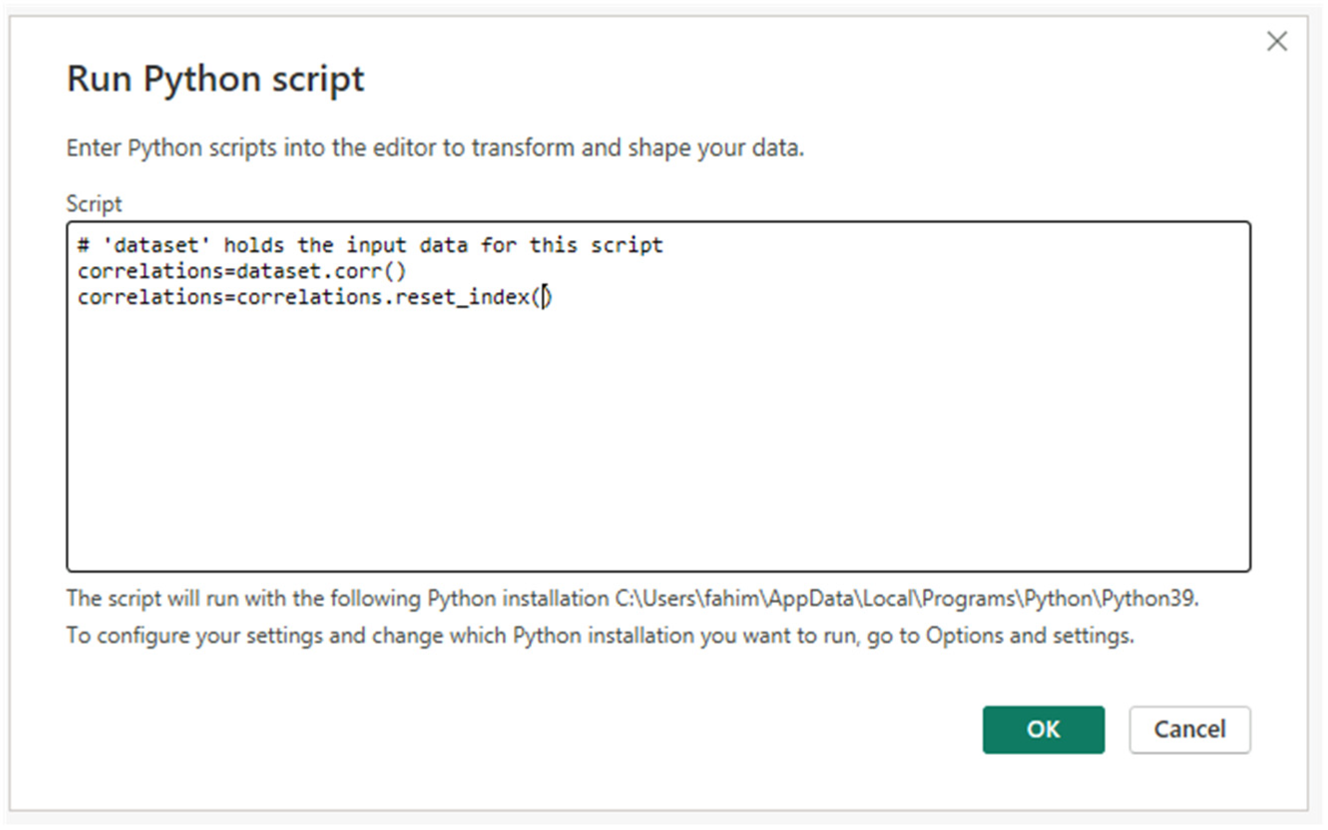
• Correlation and interdependency insights: We unveiled significant correlations between specific cyber-attack dimensions, particularly highlighting a notable correlation (coefficient of 0.93) between on-demand scan and local infection. Subsequent linear regression provided insights into their interdependency.
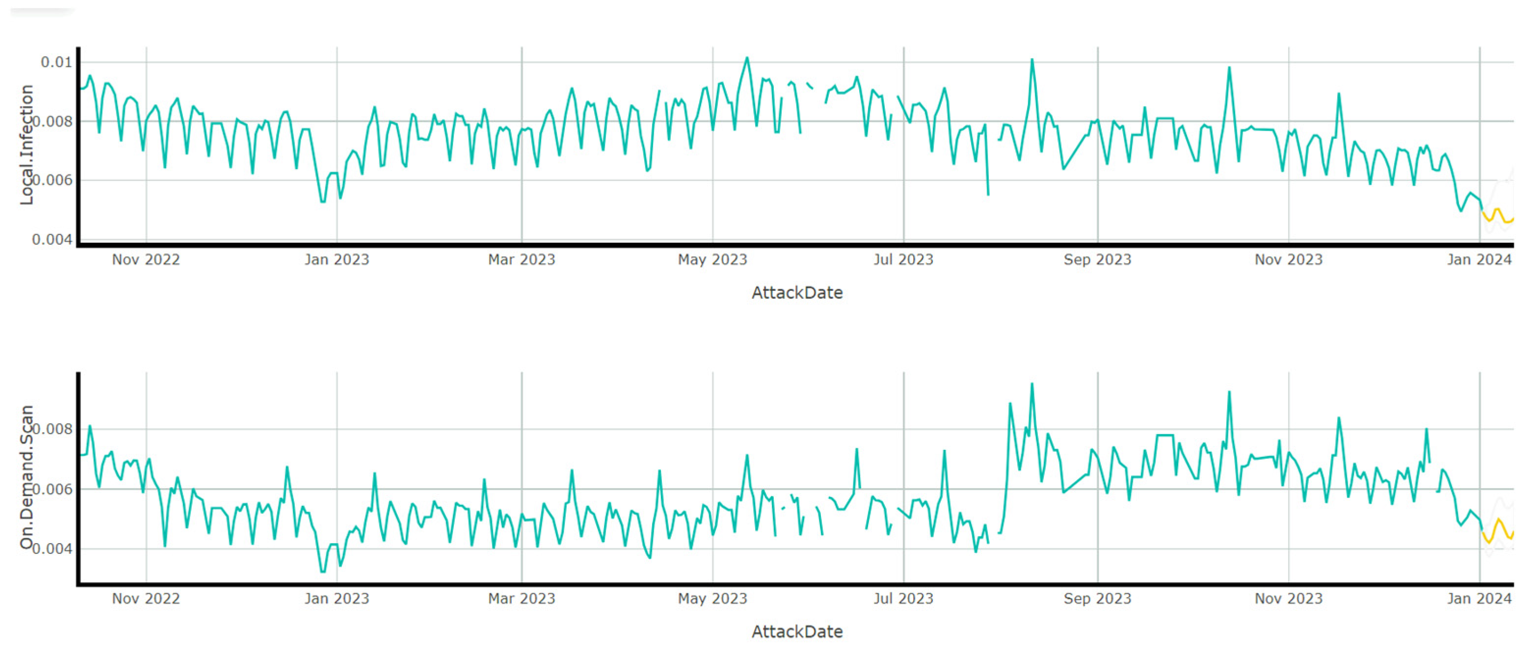
• Neural-network-based forecasting: We applied neural-network-based forecasting to predict temporal patterns of highly correlated cyber threat dimensions (on-demand scan and local infection), achieving a high level of predictive accuracy with mean squared error (MSE) and mean absolute percentage error (MAPE) values of 1.616 and 80.13, respectively.
• Practical applicability: We positioned the research within the realm of practical cybersecurity applications, offering valuable tools for risk assessment, strategic planning, and informed decision-making in the face of dynamic and evolving cyber threats.

In summary, this dataset represents a pivotal resource for the ongoing battle against cyber threats by releasing the most robust global cyber-attack dataset and demonstrating its use in cyber analytics and prediction (as highlighted clearly in Table 1). Its comprehensive nature, coupled with the advanced methodologies employed in its compilation and analysis, positions it as a cornerstone for future cybersecurity research. Due to the significant contributions of both releasing a robust global cyber dataset and enhancing analytical capabilities for the prediction of cyber threats, they will be emphasized in the subsequent sections.

2. Methods

The methodology employed in the aggregation and collation of this comprehensive cyber dataset leverages a combination of modern low-code tools and AI-based robotic process automation (RPA), ensuring both efficiency and accuracy in data collection and processing [16]. This section details the methods applied for data collection, treatment, validation, and curation, along with notes on data quality and noise.

2.1. Data Collection and Treatment

2.1.1. Automated Data Collection

The data collection process was initiated through Microsoft Power Automate [30], which scheduled a cloud flow to trigger an unattended Microsoft Power Automate Desktop flow. This setup allowed for the autonomous operation of a pre-configured Azure virtual machine, even when signed out, thereby facilitating continuous data collection. The Microsoft Power Automate Cloud Flow (highlighted as step 1 in Figure 1), in a completely autonomous manner, logs in to a Microsoft Azure remote machine at 6:00 a.m. every morning. As seen from Figure 2, the cloud flow autonomously operates for 20 to 30 min and during this time requests, queues, assigns, connects, and executes, before finally logging out (i.e., finalizes) of the remote machine. The cloud flow seen in Figure 2, calls for a sequence of steps (i.e., RPA) within the Microsoft Azure virtual machine (i.e., remote machine). This machine has Microsoft Power Automate Desktop installed, which carries out all the sequential RPA steps.

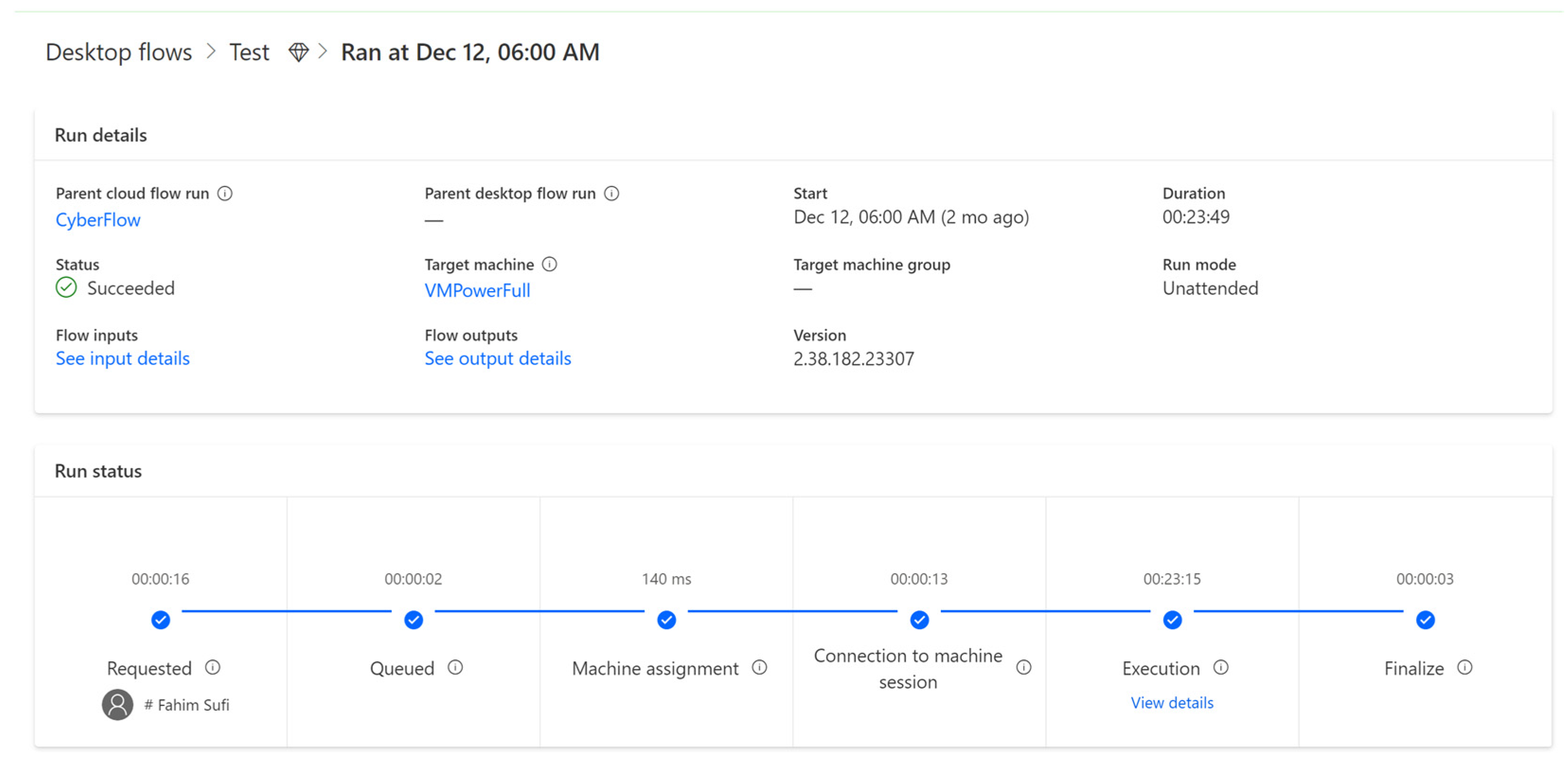
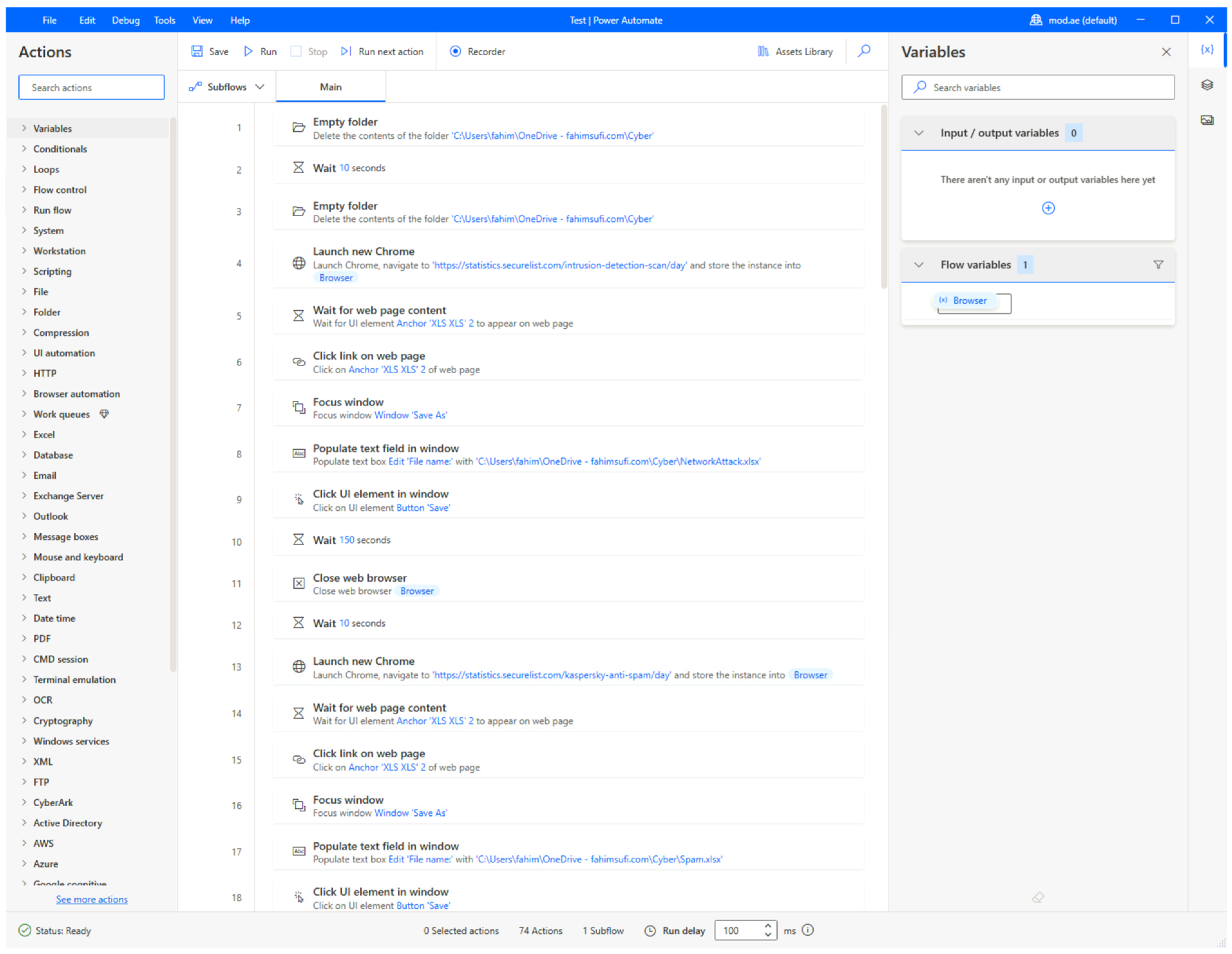
2.1.2. Robotic Process Automation

As Microsoft Power Automate Cloud Flow initiates the remote machine (as seen in Figure 2), it also logs in to this remote machine as an admin user. After logging in as an admin user, a series of RPA tasks are executed. As seen from Figure 3, these tasks involve reaching eight different sites, clicking the appropriate button to initiate a download, renaming the files (e.g., NetworkAttack.xls, Spam.xls, etc.), and saving them in Microsoft One Drive. Within the RPA tasks of Microsoft Power Automate Desktop, as shown in Figure 3, the task called “Launch New Chrome” launches the Chrome browser in an automated manner and points to the appropriate URLs from the eight different web links [4,5,6,7,8,9,10,11,12]. The task “Wait for web page content” allows the process to stall until the page content of the cyber statistics loads completely. Then, the download button is clicked with “Click link on web page” task. Next, “Focus window” focuses on the “Save As” window for renaming the files. The RPA task “Populate text field in window” enters the new file name in order to save them inside a Microsoft OneDrive for Business folder location. The modern RPA routines demonstrated in this method (i.e., Figure 3) use several AI-based techniques [31,32] for locating items (such as download buttons, or items or links) through computer vision. These RPA’s can perform optical character recognition (OCR) in order to locate download links from images, mimicking the manual actions of humans [33]. In the context delineated by step 2 of Figure 1, OCR, denoting image processing, serves the purpose of identifying a download button’s whereabouts and effectuating its activation automatically to commence the download process.

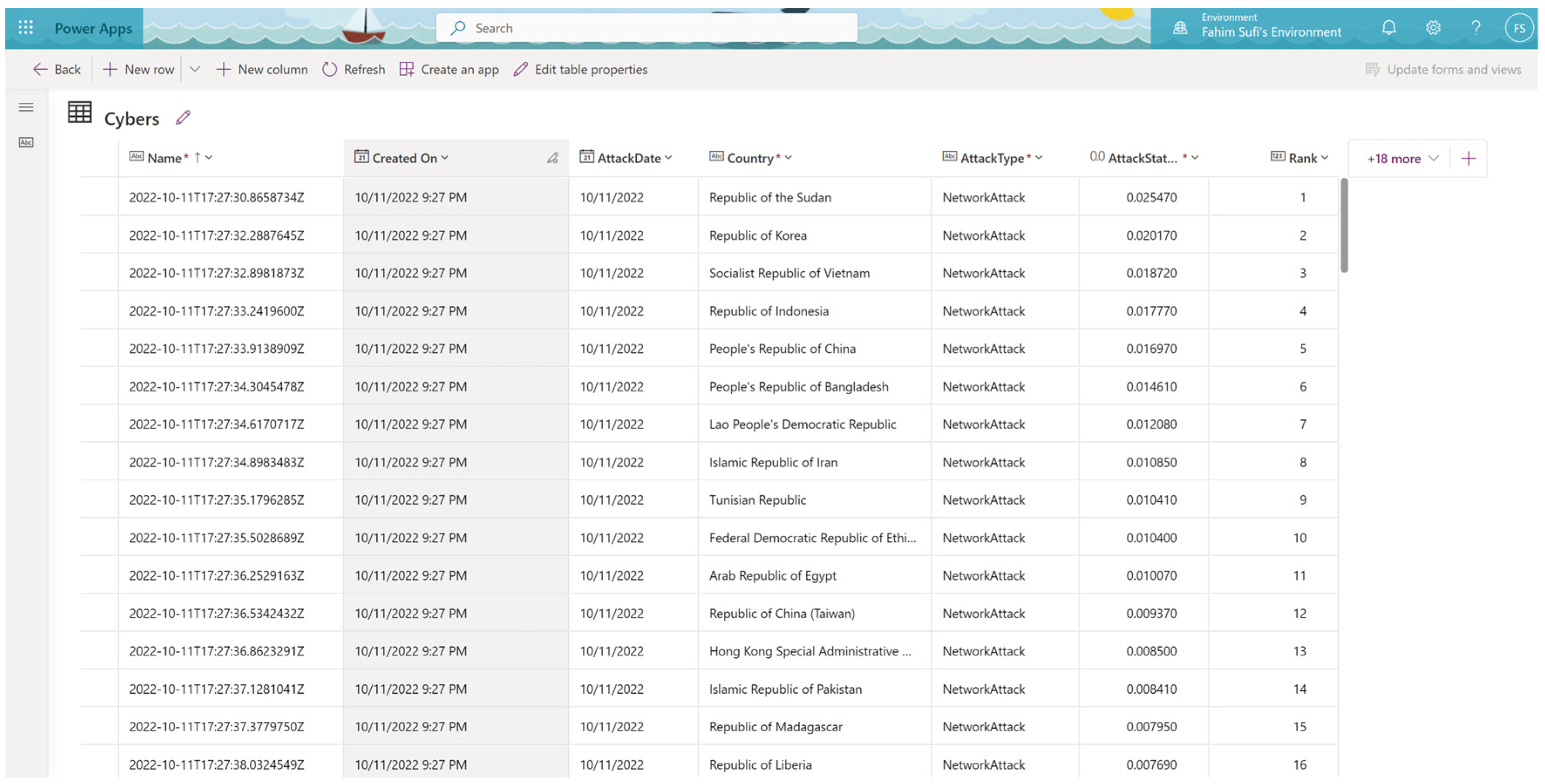
2.1.3. Data Storage and Integration

Upon the deposition of files in the OneDrive folder, another Microsoft Power Automate Cloud Flow becomes activated. This flow processes the files and stores the data permanently in Microsoft Dataverse [34], ensuring secure and organized data management. Figure 4 shows several of these cyber-attack statistics by date, country, attack type, percentage of attack, and ranking of cyber-attack. It should be noted that the time-series compilation of cyber-attack statistics was possible because of the methodological and well-orchestrated employment of automations tools like Microsoft Power Automate Cloud Flow, Microsoft Power Automate Desktop Flow, Microsoft One Drive, and Microsoft Dataverse. While Figure 3 represents the disposition of files containing single attack type data for a single day, Figure 4 presents aggregated time-series data across multiple days, and multiple attack types. As clearly seen from Figure 4, the rank column provides rankings based on the AttackStatistics (i.e., percentage of attack) for a particular day on a particular attack type.

2.1.4. Data Manipulation and Analysis

The final step involved using Microsoft Power BI [35], equipped with Data Analysis Expressions (DAX) and Power Query. This tool was instrumental in manipulating the data, performing AI-based analysis, and visualizing the time-series cyber data. The final dataset comprised 77,623 rows and 18 columns.

Within this step, DAX and Power Query transposes the attack-type (i.e., percentage values of the eight different attack types) and rank (ranking of the eight different attack types) columns. Thus, Figure 4 is turned into Figure 5 using Microsoft Power BI. As seen in Figure 5, the final data columns compose of the attack date and country of Figure 4 with the addition of eight attack percentages columns (i.e., spam, ransomware, local infection, exploit, malicious mail, network attack, on-demand scan, web threat etc.) and eight attack ranking columns (i.e., eighteen columns in total). The corresponding DAX code to perform this data transformation is provided in Appendix A.

2.2. Validation and Curation

• Automated process monitoring: The automated data collection process was closely monitored. It was noted that, for 17 days of the 14-month period, the process was interrupted due to essential updates required by the Azure Virtual Machine or Power Automate Desktop. These interruptions were promptly addressed to minimize data loss.
• Data integrity checks: Regular integrity checks were performed to ensure the accuracy and completeness of the data collected. This involved verifying the data against secondary sources and conducting random sample checks. It should be mentioned that the same methodology was implemented on another virtual machine for ensuring business continuity. In case of the unavailability of one virtual machine (due to maintenance or any other reasons), the other virtual machine would be automatically utilized.

2.3. Data Quality and Noise

• Noise reduction: Efforts were made to reduce noise and irrelevant information during the data collection phase. This was achieved through the careful configuration of the RPA scripts to selectively download relevant data.
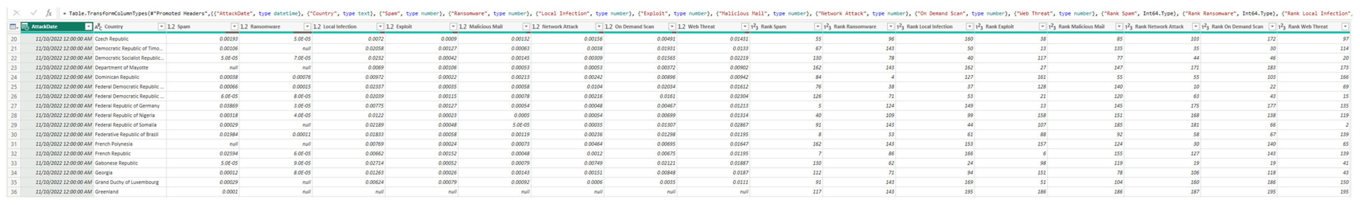
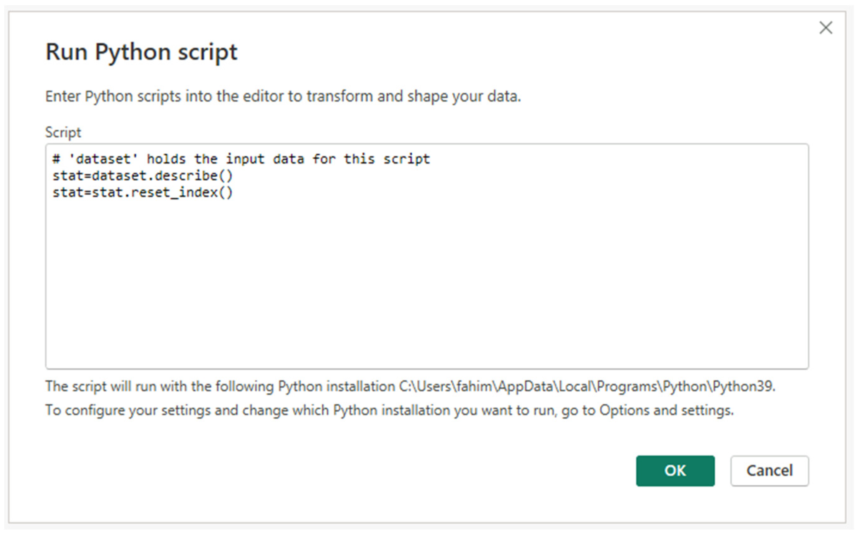
• Quality assurance and data cleaning: The quality of the data was maintained through rigorous validation protocols. In the data manipulation phase, Power BI was used to clean the dataset. This involved removing duplicates, correcting inconsistencies, and handling missing values, thereby enhancing the quality and usability of the dataset. For example, an automated script replaced the null values (as seen in Figure 5) with 0.

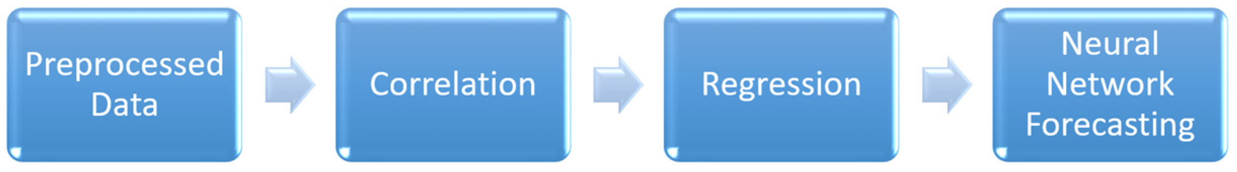
2.4. Data Analysis and Forecasting

After validating the data quality, the data are fed through a three-step process as shown in Figure 6, beginning with correlation.

The correlation matrix, being the output of the correlation process, shows all of the cyber-parameters that are highly correlated. The values of the correlation coefficients range from −1 to 1, with the following insights:

• 1: A perfect positive correlation, meaning that, as one variable increases, the other variable also increases proportionally.
• 0: No correlation, indicating that there is no linear relationship between the variables.
• −1: A perfect negative correlation, signifying that, as one variable increases, the other variable decreases proportionally.

The correlation matrix is a symmetric matrix, as the correlation between Variable A and Variable B is the same as the correlation between Variable B and Variable A. For a set of variables {X₁, X₂, …, X_n}, the correlation matrix might look like Equation (1).

$$Correlation Matrix=\left|\begin{array}{ccc}1& \cdots & r_{1n}\\ \cdots & \ddots & \cdots \\ r_{n1}& \cdots & 1\end{array}\right|$$

(1)

where r_ij represents the correlation coefficient between X_i and X_j. The diagonal elements (e.g., r₁₁, r₂₂, …, r_nn) are always 1 because a variable has a perfect correlation with itself. Correlation matrices are commonly used in statistics, finance, and other fields to explore relationships between variables, identify patterns, and understand the interdependencies within a dataset.

As seen from Figure 6, once the correlation step is complete, regression is performed on the cyber-threat data. A linear regression identifies the linear relationship between the dependent and independent variables in the form of Equation (2).

$$y=b_0+b_1{x}_1+\epsilon$$

(2)

The process ends with the forecasting of related parameters using a neural network. Equation (3) shows an autoregressive model in the order of p, where h(.) is a nonlinear function. Here, ${\epsilon }_t$ is a sequence of random independent parameters with the distribution of zero mean and finite variance σ². An autoregressive neural network is shown in Equations (4) and (5) as a feed-forward network. The f(.) function is an activation function with a parameter vector of $\theta =({\beta }_0, {\beta }_1, \dots , {\beta }_q, {\alpha }_1, \dots , {\alpha }_q, {\omega }_{11}, \dots , {\omega }_{qn})$.

$$y_t=h\left(y_{t-1}, \dots , y_{t-p}\right)+{\epsilon }_t$$

(3)

$${\widehat{y}}_t=\widehat{h}(y_{t-1}, \dots , y_{t-p})$$

(4)

$${\widehat{y}}_t={\beta }_0+\sum _{i=1}^I{\beta }_{j}f({\alpha }_i+\sum _{j=1}^p{w}_{ij}{y}_{t-j})$$

(5)

Equation (6), on the other hand, shows a generalized linear model in a nonlinear case, with h(.) being a nonlinear function and ${\epsilon }_t$ representing the same contextual information portrayed in Equation (5). As shown in Equations (7) and (8), ${\widehat{y}}_t$ is calculated with recursive estimation, because of the non-observational nature of ${\epsilon }_{t-1}, \dots ,{\epsilon }_{t-q}$.

$$y_t=h\left(y_{t-1}, \dots , y_{t-p}, {\epsilon }_{t-1}, \dots ,{\epsilon }_{t-q}\right){+\epsilon }_t$$

(6)

$${\widehat{y}}_t=h\left(y_{t-1}, \dots , y_{t-p}, {\widehat{\epsilon }}_{t-1}, \dots ,{\widehat{\epsilon }}_{t-q}\right)$$

(7)

$${\widehat{\epsilon }}_t=y_{t-1}-{\widehat{y}}_j, j=t-1, \dots t-q$$

(8)

The recurrent neural network model can now be expressed with a recurrent network, as defined in Equations (9) and (10).

$${\widehat{y}}_t=a_0+{\sum }_{j=1}^h{a}_{j}g({\beta }_{0j})+{\sum }_{i=1}^p{\beta }_{ij}{y}_{t-i}+{\sum }_{i=p+1}^{p+q}{\beta }_{ij}{\widehat{\epsilon }}_{t+p-i}$$

(9)

$${\widehat{\epsilon }}_{t+p-i}=y_{t+p-i}-{\widehat{Y}}_{t+p-i}$$

(10)

In conclusion, the methodological framework applied in this study harnesses the power of modern low-code tools, AI-driven automation, and AI-driven analytics. As summarized in

Table 2. The use of various technology components for fulfilling functional requirements (⚫ = Supported).

Technology Component	Automate Data Acquisition	Correlation	Regression	Neural-Network-Based Forecasting	Deployment in iOS, Android, and Windows Devices
Microsoft Power Automate Desktop	⚫
Microsoft Power Automate Cloud Flow	⚫
Microsoft One Drive	⚫
Microsoft Dataverse	⚫
Microsoft Power BI Desktop		⚫	⚫	⚫	⚫
Python on Power BI		⚫	⚫	⚫	⚫
Microsoft Power BI Service					⚫

and shown in Figure 1, Microsoft Power Automate Desktop, Microsoft Power Automate Cloud Flow, Microsoft One Drive, Microsoft Dataverse, and Microsoft Power BI were used to automate the cyber-threat data acquisition process. Correlation, regression and a neural network were implemented with Python (shown in Appendix A). Finally, the entire solution was deployed and tested in multiple platforms and devices covering Windows, iOS, and Android. This approach not only streamlined the data collection process but also ensured the high quality and reliability of the dataset, making it a valuable resource for cybersecurity research.

3. Results

The dataset, encompassing a broad spectrum of cyber-attack dimensions, consists of 77,623 rows and 18 fields, as shown in

Table 3. Data types and descriptions for all of the 18 fields, with sample data (# means number).

Field Name	Data Type	Valid #	Valid %	Error #	Error %	Empty #	Empty %	Sample Data
Attack date	Date	77,623	100%	0	0%	0	0%	25 April 2023
Country	Text	77,623	100%	0	0%	0	0%	Bangladesh
Spam	Decimal	62,982	81%	0	0%	14,641	19%	0.01358
ransomware	Decimal	52,144	67%	0	0%	25,479	33%	0.00025
Local infection	Decimal	74,469	96%	0	0%	3154	4%	0.00726
Exploit	Decimal	64,264	83%	0	0%	13,359	17%	0.00021
Malicious mail	Decimal	69,184	89%	0	0%	8439	11%	0.00019
Network attack	Decimal	71,532	92%	0	0%	6091	8%	0.00076
On-demand scan	Decimal	74,231	96%	0	0%	3392	4%	0.00445
Web threat	Decimal	73,892	95%	0	0%	3731	5%	0.01116
Rank spam	Text	77,623	100%	0	0%	0	0%	34
Rank ransomware	Text	77,623	100%	0	0%	0	0%	6
Rank local infection	Text	77,623	100%	0	0%	0	0%	100
Rank exploit	Text	77,623	100%	0	0%	0	0%	108
Rank malicious mail	Text	77,623	100%	0	0%	0	0%	56
Rank network attack	Text	77,623	100%	0	0%	0	0%	94
Rank on-demand scan	Text	77,623	100%	0	0%	0	0%	109
Rank web threat	Text	77,623	100%	0	0%	0	0%	109

. Table 3 also shows sample data (row 37,349 of the Supplementary Materials). Each field’s statistical distribution, along with 25th, 50th, and 75th percentiles are detailed in

Table 4. Data distributions and statistics of for the eight cyber-attack percentage (i.e., decimal) fields.

Index	Spam	Ransomware	Local Infection	Exploit	Malicious Mail	Network Attack	On-Demand Scan	Web Threat
min	0.00001	0.00001	0.00024	0.00001	0.00001	0.00002	0.00024	0.00024
25%	0.00009	0.00004	0.00715	0.00021	0.0003	0.0007	0.00521	0.0097
50%	0.00059	0.00007	0.01079	0.00039	0.00073	0.00129	0.00814	0.01257
75%	0.00353	0.00014	0.01766	0.00062	0.00169	0.00235	0.01287	0.015973
max	0.30249	0.00918	0.04937	0.00466	0.04322	0.05826	0.12488	0.04863
mean	0.006094	0.00013	0.01335	0.000469	0.001292	0.002222	0.009756	0.013006
std	0.024337	0.000186	0.008415	0.000368	0.001606	0.003034	0.00608	0.004943
count	62,982	52,144	74,469	64,264	69,184	71,532	74,231	73,892

and

Table 5. Data distributions and statistics of for the eight cyber-attack rankings (i.e., Text) fields.

Index	Rank Spam	Rank Ransomware	Rank Local Infection	Rank Exploit	Rank Malicious Mail	Rank Network Attack	Rank On-Demand Scan	Rank Web Threat
min	1	1	1	1	1	1	1	1
25%	48	41	47	38	48	48	47	46
50%	98	88	98	90	98	98	97	97
75%	144	131	148	144	147	148	148	148
max	186	158	196	188	194	192	196	196
mean	94.53299	84.00165	97.73	90.46	96.80494	97.76224	97.42858	96.97435
std	52.67272	48.97654	58.05	58.98	55.90629	56.90058	58.17745	58.45481
count	77,623	77,623	77,623	77,623	77,623	77,623	77,623	77,623

, providing a comprehensive overview of the global cyber threat landscape.

• Attack date (date): Records the date of each cyber-attack. All 77,623 entries are valid, indicating a complete dataset with no missing dates (as shown in Table 3).
• Country (text): Specifies the country of the cyber-attack occurrence. All entries are valid, covering 225 countries, and provide a global perspective on cyber threats (as shown in Table 3).
• Spam (decimal): Records the percentage of spam-related attacks for a specific country on a particular day (percentage value in decimal). The sample data, as shown in Table 3, for spam is 0.01358, meaning that Bangladesh suffered 1.358% of spam attacks on that day. With 62,982 valid entries, the mean is 0.006094, and the standard deviation is 0.024337. The range is from a minimum of 0.000010 to a maximum of 0.302490. The 25th, 50th, and 75th percentiles are 0.000090, 0.000590, and 0.003530, respectively (as shown in Table 3 and Table 4).
• Ransomware (decimal): Records the percentage of ransomware related attacks for a specific country on a particular day. This consists of 52,144 valid entries (Table 3). As per Table 4, the average value is 0.000130, with a standard deviation of 0.000186. The range spans from 0.000010 to 0.009180. The percentiles are 0.000040 (25th), 0.000070 (50th), and 0.000140 (75th).
• Local infection (decimal): Records the percentage of local infections for a specific country on a particular day. With 74,469 entries, the mean is 0.013350, and the standard deviation is 0.008415. The values range from 0.000240 to 0.049370. The percentiles are 0.007150 (25th), 0.010790 (50th), and 0.017660 (75th) (detailed in Table 3 and Table 4).
• Exploit (decimal): Records the percentage of exploit-related attacks for a specific country on a particular day. Contains 64,264 valid entries. The mean is 0.000469, with a standard deviation of 0.000368. The range is from 0.000010 to 0.004660. The 25th, 50th, and 75th percentiles are 0.000210, 0.000390, and 0.000620, respectively (shown in Table 3 and Table 4).
• Malicious mail (decimal): Records the percentage of malicious-mail-related attacks for a specific country on a particular day. Comprises 69,184 entries. The mean is 0.001292, with a standard deviation of 0.001606. The range spans from 0.000010 to 0.043220. The percentiles are 0.000300 (25th), 0.000730 (50th), and 0.001690 (75th) (Table 3 and Table 4).
• Network attack (decimal): Records the percentage of network-attack-related incidents for a specific country on a particular day. With 71,532 entries, the average value is 0.002222, and the standard deviation is 0.003034. The range is from 0.000020 to 0.058260. The 25th, 50th, and 75th percentiles are 0.000700, 0.001290, and 0.002350, respectively (shown in Table 3 and Table 4).
• On-demand scan (decimal): Records the percentage of on-demand scans (by the anti-virus program) for a specific country on a particular day. This contains 74,231 valid entries. The mean is 0.009756, with a standard deviation of 0.006080. The minimum and maximum values are 0.000240 and 0.124880, respectively. The percentiles are 0.005210 (25th), 0.008140 (50th), and 0.012870 (75th) (detailed in Table 3 and Table 4).
• Web threat (decimal): Records the percentage of web-threat-related attacks for a specific country on a particular day. This comprises 73,892 entries. The mean value is 0.013006, with a standard deviation of 0.004943. The range spans from 0.000240 to 0.048630. The 25th, 50th, and 75th percentiles are 0.009700, 0.012570, and 0.015973, respectively (shown in Table 3 and Table 4).
• 11–18. Rank fields (text): These fields (rank spam, rank ransomware, rank local infection, rank exploit, rank malicious mail, rank network attack, rank on-demand scan, and rank web threat) provide the world ranking of each country in the respective cyber-attack dimension. The rankings range from 1 to a maximum of 196, with the mean rankings varying slightly across different attack types. The standard deviation in these rankings indicates a moderate spread, reflecting the varying impact of cyber threats across different countries (as detailed in Table 3 and Table 4).

In summary, the dataset offers a detailed and comprehensive view of cyber threats across multiple dimensions. The statistical analysis reveals the varying intensity and frequency of different types of cyber-attacks, providing valuable insights for researchers and policymakers. The complete and valid entries for the attack date and country fields ensure a robust temporal and geographical representation of the data. Figure 7 shows the new dataset driving a cyber-intelligence solution within an Android deployment on the latest Samsung Galaxy S23 Mobile. As seen from Figure 7, a particular time period (i.e., from 1 November 2022 to 8 March 2023) was selected for Australia. As seen from the spider chart on the mobile environment, Australia suffers most critically from web threats (1st), local infections (2nd), on-demand scan (3rd), spam (4th) and then the other cyber-attack dimensions. Any other countries within the globe can be selected by the user, and the mobile-based solution (available in iOS, Android, and Windows) could empower the cyber analyst with interactive insights on threat dimensions, threat ranking, threat patterns, and event forecasting. Unlike existing research works that have used network traffic data (that is applicable to a single institute or organization) [36,37,38], the global cyber-attack data generated in this research facilitates comparative analytics among multiple countries. Therefore, national leaders, cyber strategists, and policymakers can use an intelligent system like that shown in Figure 7 on their mobile devices, facilitating just-in-time decisions on national cyber postures.

Figure 8 depicts the correlations among the eight different types of cyber-attack dimensions (i.e., exploit, local infection, malicious mail, network attack, on-demand scan, ransomware, spam and web threat). As previously shown in Equation (1), the correlation coefficient, denoted as “r”, quantifies the strength and direction of a linear relationship. As seen in Figure 8, there is a correlation coefficient value of 0.93 between on-demand scan and local infection, which indicates a very strong positive linear relationship between these variables. As these variables (on-demand scan and local infection) are linearly related, linear regression (i.e., as shown previously in Equation (2)) can be used to quantify the relationship. As shown previously in Equation (2), given a value of X, the model predicts the corresponding value of Y based on the regression equation (as seen from Figure 9). The linear regression model can be used for prediction.

Finally, Figure 10 shows the prediction of both on-demand scan and local infection for Australia. As seen from Figure 10, the trends, patterns, seasonality for both these cases appear to be similar, since earlier experimentation found that both these factors (i.e., on-demand scan and local infection) are highly correlated, with a correlation coefficient of 0.93. Though Figure 10 only showcases predictions for on-demand scan and local infection (as these were found to be correlated), predictions could be generated seamlessly for all of the eight cyber-attack dimensions, for a more comprehensive understanding of future threats. For predicting time-series data there are some popular methods, like exponential smoothing [39], autoregressive integrated moving average (ARIMA) [40], and neural networks [40,41]. In our previous research, an exponential smoothing algorithm was used to predict cyber-attacks from time-series data [13,14,15] using Microsoft Power BI implementation. However, in this study neural-network-based forecasting was implemented with Python code within a Microsoft Power BI environment. This could also be executed using the visuals produced by MAQ Software, Redmond, WA, USA, following the implementation guidelines of [42]. Appendix A showcases the python code that was executed within a Microsoft Power BI environment. This code predicted cyber-attacks for 10 days with an 80% confidence level.

Although the aggregation process for this dataset is intricate, utilizing various features of modern AI-driven tools, the study’s resulting data are stored in a simple and easy-to-use CSV file format (publicly accessible at https://github.com/DrSufi/CyberData, accessed on 14 February 2024).

4. Discussion

While there are several cyber intelligence solutions [43,44,45,46,47] that portray global cyber threat statistics, none of these solutions provide access to time-series cyber statistics data. This research uses an innovative AI-driven RPA methodology to acquire, manage, and store global cyber threat statistics. The presented methodology of data aggregation is fully automated and much more robust in comparison with existing systems [48,49,50,51,52]. The comprehensive cyber data deriving from this study have been made available to researchers and academics for the first time in order to facilitate open-source cyber research. This dataset could be used to identify correlations [20,21], for regression [17,18,19], and for prediction. The dataset, meticulously compiled from various open-source statistics, and employing modern AI techniques for data treatment and analysis, includes sensitive dimensions of cyber-attacks but does not contain individual or personally identifiable information. This is because Kaspersky [4] tracks the cyber-attack data at country level (i.e., not a personal level).

4.1. Use of This Dataset

This section provides essential guidance for researchers and analysts intending to utilize the dataset. The section aims to facilitate efficient and effective use of the data, ensuring that users can quickly familiarize themselves with its structure and nuances.

• Date format and chronological analysis: The ‘Attack-Date’ field is crucial for any time-series analysis. Users should ensure that their analytical tools correctly interpret the date format for accurate temporal analysis.
• Handling missing values: Fields such as spam, ransomware, and others contain empty entries, representing days with no recorded activities. Users should decide on their approach to handling these missing values based on their research objectives, i.e., whether to treat them as zeros, ignore them, or use imputation techniques.
• Statistical analysis: The dataset provides rich ground for statistical analysis, with fields showing varying degrees of standard deviation and range. Users should consider appropriate statistical methods to analyze these fields, keeping in mind the distribution characteristics like mean, median, percentiles, and range.
• Comparative and ranking analysis: The rank fields offer a unique opportunity for comparative analysis across countries and cyber-attack dimensions. Researchers interested in global or regional comparisons will find these fields particularly useful.
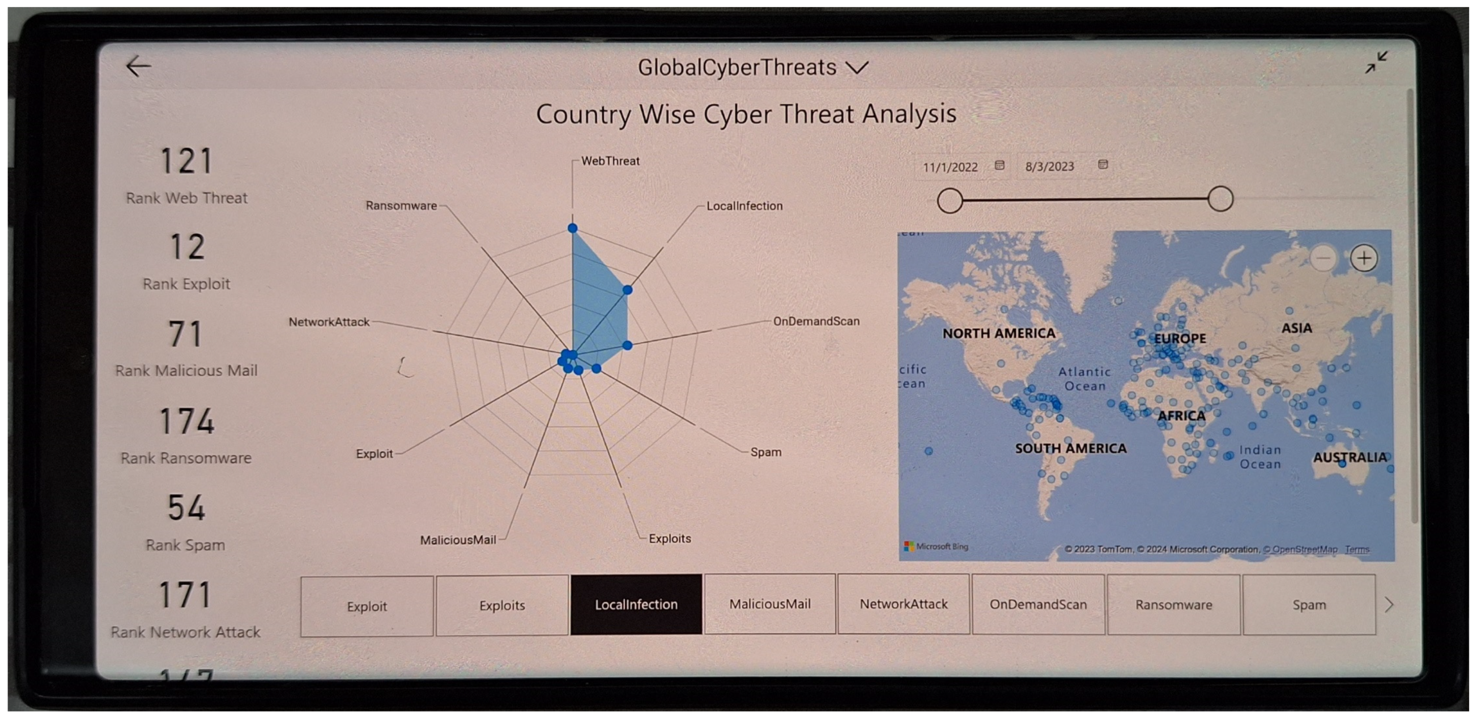
• Data visualization: Given the dataset’s complexity and breadth, effective visualization tools (like Microsoft Power BI used in its creation) are recommended for a more intuitive understanding of trends and patterns.
• Cross-referencing with external data: Users are encouraged to augment this dataset with external data sources for more comprehensive analysis (e.g., [15]). This could include socio-economic data, digital infrastructure metrics, or other relevant datasets.
• Ethical considerations: While the dataset does not contain personal data, users should still adhere to ethical guidelines in their analysis, particularly when publishing results or drawing conclusions that might influence public policy or perception.
• Updates and version control: Users should note that the dataset covers up to December 2023. Any developments in the cyber threat landscape post this period will not be reflected. Keeping track of dataset versions and updates is crucial for longitudinal studies.
• Collaboration and sharing findings: Users are encouraged to share their findings with the broader research community. Collaboration can lead to more robust insights and a deeper understanding of the global cyber threat landscape.

4.2. Performance Evaluation

As seen from

Table 6. Performance evaluation of the neural-network-based cyber-threat prediction.

Country	Attack Type	MSE	MAPE (%)
Australia	Local infection	1.45	79.2%
Australia	On-demand scan	1.85	88.4%
New Zealand	Local infection	1.72	83.1%
New Zealand	On-demand scan	1.55	81.3%
Saudi Arabia	Local infection	1.32	71.7%
Saudi Arabia	On-demand scan	1.39	72%
UAE	Local infection	1.68	80.3%
UAE	On-demand scan	1.71	82.9%
Qatar	Local infection	1.66	78.5%
Qatar	On-demand scan	1.73	83.9%

, the performance of the forecasting algorithm using a neural network was computed for several countries (e.g., Australia, New Zealand, Saudi Arabia, UAE, Qatar). It should be mentioned that the presented system empowered with the presented time-series would support cyber-threat forecasting for any countries on any of the threat dimensions. However, for the performance evaluations, few countries were randomly selected. The justification for choosing local infection and on-demand scan is that, in our earlier experimentation, we observed that these two dimensions were correlated. For performance metrics, we used mean square error (MSE) and mean absolute percent error (MAPE), as shown in Table 6. With A_t being actual threat and F_t being the forecasted threat for time t, MSE and MAPE could be represented with Equations (11) and (12).

$$MSE=\frac{1}{n}\sum _t^n{(A_t-F_t)}^2$$

(11)

$$MAPE =\frac{100}{n}{\sum }_{t=1}^n\frac{\left|A_t-F_t\right|}{\overline{X}}$$

(12)

As seen from Table 6, the mean of MSE was found to be 1.616 ± 0.2446 (where, 1.616 was the mean, μ and 0.2446 was the standard deviation, σ of the MSE). Similarly, MAPE was found to be 80.13 ± 4.9742%. The highest value of MSE/MAPE was recorded for Australia on on-demand scan and the lowest value of the MSE/MAPE was identified for Saudi Arabia’s local infection. Hence, the accuracy of predictions showcased with this considerably extended dataset markedly surpasses that of existing studies [22,23,24,25,26,27,28,29].

4.3. Limitations of This Study

In order to obtain evidence-based policy and strategic decision-making on cyber related issues, the decision-makers use global cyber threat maps like those in [43,44,45,46,47]. Ideally, in order to take evidence-based policy decisions, decision makers should cross reference with other data sources. As of the time of writing this paper, none of these cyber intelligence solutions provide access to historical cyber-attack data (i.e., time-series) at a national level. Hence, this study used an innovative methodology to capture historical cyber data using daily cyber-threat statistics from Kaspersky [45]. Due to data inaccessibility and unavailability, this study could not cross reference the time-series dataset generated in this study with other datasets, such as those in [43,44,46,47]. That is why it is imperative that researchers and policymakers should cross-reference this dataset with other available sources (as previously suggested in Section 4.1).

Another limitation of this study is that it does not use taxonomies for the generation of a comprehensive understanding of the data. When cyber-attacks are targeted at individual agencies or institutions, researchers need to comprehend the attack through the lenses of taxonomies or frameworks [53]. Taxonomies, like those of [53], would allow a researcher to comprehend multiple dimensions like attack target, operational impact, informational impact etc. However, when comparing cyber-attacks at the country or national level, operational impacts and informational impacts, along with other dimensions of the taxonomy, become aggregated. As a result, a taxonomy, like that of [53], has limited value for comparing country level cyber-threats. Hence, almost all of the modern country-level threat intelligence providers (e.g., [43,44,45,46,47]) portray country-level threats with respect to cyber-attack types (e.g., spam, network attack, web-threat, ransomware etc.).

5. Conclusions

This study introduces an innovative automated methodology for the systematic collection of global cyber-attack data, resulting in the creation of a comprehensive dataset spanning 225 countries over a 14-month period from October 2022 to December 2023. The dataset, encompassing 77,623 rows and 18 fields, intricately delineates cyber-attacks across eight critical dimensions: spam, ransomware, local infection, exploit, malicious mail, network attack, on-demand scan, and web threat. Additionally, the dataset incorporates ranking data, affording a nuanced comparative analysis of countries’ susceptibilities to distinct cyber threats. The findings of the analysis illuminate discernible disparities in the frequency and intensity of cyber-attacks, both across different countries and within varying attack types. A correlation analysis underscores a noteworthy correlation (coefficient of 0.93) between on-demand scan and local infection. Subsequent linear regression between these correlated dimensions serves to elucidate their interdependency. An avant-garde application of neural-network-based forecasting is employed to predict the temporal patterns of on-demand scan and local infection. The predictive model demonstrates a notable precision, substantiated by mean squared error (MSE) and mean absolute percentage error (MAPE) values of 1.616 and 80.13, respectively.

Beyond the releasing of comprehensive cyber data for the first time (facilitating open-source cyber research), the practical ramifications of this research are manifold. This study offers actionable intelligence for cybersecurity strategies and strategic planning through the discernment of correlation and predictive patterns pertaining to specific cyber threat dimensions. As such, this study constitutes a substantial contribution to the evolving field of cybersecurity, providing valuable tools for risk assessment and informed decision-making in the face of the ever-evolving cyber landscape.

Future endeavors of this research direction would involve using more robust techniques to capture live cyber threat statistics from a diverse range of sources, like [43,44,46,47] the use of AI, computer vision, and RPA. This would create a more robust global cyber-attack dataset. After compiling a more robust global cyber-attack dataset, we envision the creation of a generic fit-for-purpose taxonomy in order to address the myriad dimensions of global cyber threats and use innovative transformer technology [54].

References

- Cremer, F.; Sheehan, B.; Fortmann, M.; Kia, A.N.; Mullins, M.; Murphy, F.; Materne, S. Cyber risk and cybersecurity: A systematic review of data availability. Geneva Pap. Risk Insur.-Issues Pract. 2022, 47, 698–736. [Google Scholar] [CrossRef] [PubMed]
- Cybercrime Magazine. Cybercrime to Cost the World $10.5 Trillion Annually by 2025. 2020. Available online: https://cybersecurityventures.com/hackerpocalypse-cybercrime-report-2016/ (accessed on 15 October 2022).
- Bada, J.R.N.M. Chapter 4—The social and psychological impact of cyberattacks. In Emerging Cyber Threats and Cognitive Vulnerabilities; Academic Press: Cambridge, MA, USA, 2020; pp. 73–92. [Google Scholar]
- Kaspersky. Cyber Threat Statistics. 2023. Available online: https://statistics.securelist.com/ (accessed on 3 August 2023).
- Kaspersky. Daily Spam Cyber Threat Statistics. 2023. Available online: https://statistics.securelist.com/kaspersky-anti-spam/day (accessed on 11 November 2023).
- Kaspersky. Daily Ransomware Cyber Threat Statistics. 2023. Available online: https://statistics.securelist.com/ransomware/day (accessed on 11 November 2023).
- Kaspersky. Daily Local Infections Cyber Threat Statistics. 2023. Available online: https://statistics.securelist.com/on-access-scan/day (accessed on 3 August 2023).
- Kaspersky. Daily Exploit Cyber Threat Statistics. 2023. Available online: https://statistics.securelist.com/vulnerability-scan/day (accessed on 11 November 2023).
- Kaspersky. Daily Mailicious Mail Cyber Threat Statistics. 2023. Available online: https://statistics.securelist.com/mail-anti-virus/day (accessed on 3 August 2023).
- Kaspersky. Daily Network Attack Cyber Threat Statistics. 2023. Available online: https://statistics.securelist.com/intrusion-detection-scan/day (accessed on 3 August 2023).
- Kaspersky. Daily On-Demand Cyber Threat Statistics. 2023. Available online: https://statistics.securelist.com/on-demand-scan/day (accessed on 3 August 2023).
- Kaspersky. Day Web Threat Cyber Threat Statistics. 2023. Available online: https://statistics.securelist.com/web-anti-virus/day (accessed on 11 November 2023).
- Sufi, F. A global cyber-threat intelligence system with artificial intelligence and convolutional neural network. Decis. Anal. J. 2023, 9, 100364. [Google Scholar] [CrossRef]
- Sufi, F. Novel Application of Open-Source Cyber Intelligence. Electronics 2023, 12, 3610. [Google Scholar] [CrossRef]
- Sufi, F. A New AI-Based Semantic Cyber Intelligence Agent. Future Internet 2023, 15, 231. [Google Scholar] [CrossRef]
- Sufi, F. Algorithms in Low-Code-No-Code for Research Applications: A Practical Review. Algorithms 2023, 16, 108. [Google Scholar] [CrossRef]
- Lalou, M.; Kheddouci, H.; Hariri, S. Identifying the Cyber Attack Origin with Partial Observation: A Linear Regression Based Approach. In Proceedings of the IEEE 2nd International Workshops on Foundations and Applications of Self* Systems (FAS*W), Tucson, AZ, USA, 18–22 September 2017. [Google Scholar]
- Cai, F.; Ozdagli, A.; Koutsoukos, X. Variational Autoencoder for Classification and Regression for Out-of-Distribution Detection in Learning-Enabled Cyber-Physical Systems. Appl. Artif. Intell. 2022, 36, 2131056. [Google Scholar] [CrossRef]
- Ghafouri, A.; Vorobeychik, Y.; Koutsoukos, X. Adversarial Regression for Detecting Attacks in Cyber-Physical Systems. In Proceedings of the International Joint Conference on Artificial Intelligence, Stockholm, Sweden, 13–19 July 2018. [Google Scholar]
- Albasheer, H.; Siraj, M.M.; Mubarakali, A. Cyber-Attack Prediction Based on Network Intrusion Detection Systems for Alert Correlation Techniques: A Survey. Sensors 2022, 22, 1494. [Google Scholar] [CrossRef]
- Pires, S.; Mascarenhas, C. Cyber Threat Analysis Using Pearson and Spearman Correlation via Exploratory Data Analysis. In Proceedings of the Third International Conference on Secure Cyber Computing and Communication (ICSCCC), Jalandhar, India, 5 May 2023. [Google Scholar]
- Werner, G.; Yang, S.; McConky, K. Time Series Forecasting of Cyber A‚ack Intensity. In Proceedings of the Cyber and Information Security Research (CISR) Conference, Oak Ridge, TN, USA, 4–6 April 2017. [Google Scholar]
- Bakdash, J.Z.; Hutchinson, S.; Zaroukian, E.G.; Marusich, L.R.; Thirumuruganathan, S.; Sample, C.; Hoffman, B.; Das, G. Malware in the future? Forecasting of analyst detection of cyber events. J. Cybersecur. 2018, 4, tyy007. [Google Scholar] [CrossRef]
- Husák, M.; Komárková, J.; Bou-Harb, E.; Celeda, P. Survey of Attack Projection, Prediction, and Forecasting in Cyber Security. IEEE Commun. Surv. Tutor. 2018, 21, 640–660. [Google Scholar] [CrossRef]
- Aflaki, A.; Gitizadeh, M.; Kantarci, B. Accuracy improvement of electrical load forecasting against new cyber-attack architectures. Sustain. Cities Soc. 2022, 77, 103523. [Google Scholar] [CrossRef]
- Alrahmani, Z.A.; Elleithy, K. DDoS Attack Forecasting Using Transformers. In Proceedings of the IEEE Intl Conf on Dependable, Autonomic and Secure Computing, Intl Conf on Pervasive Intelligence and Computing, Intl Conf on Cloud and Big Data Computing, Intl Conf on Cyber Science and Technology Congress (DASC/PiCom/CBDCom/CyberSciTech), Abu Dhabi, United Arab Emirates, 14 November 2023. [Google Scholar]
- Choi, C.; Shin, S.; Shin, C. Performance evaluation method of cyber attack behaviour forecasting based on mitigation. In Proceedings of the 2021 International Conference on Information and Communication Technology Convergence (ICTC), Jeju Island, Republic of Korea, 20 October 2021. [Google Scholar]
- Alrawi, O.; Ike, M.; Pruett, M.; Kasturi, R.P.; Barua, S.; Hirani, T.; Hill, B.; Saltaformaggio, B. Forecasting Malware Capabilities From Cyber Attack Memory Images. In Proceedings of the 30th Usenix Security Symposium, Vancouver, BC, Canada, 11–13 August 2021. [Google Scholar]
- Qasaimeh, M.; Hammour, R.A.; Yassein, M.B.; Al-Qassas, R.S.; Torralbo, J.A.L.; Lizcano, D. Advanced security testing using a cyber-attack forecastingmodel: A case study of financial institutions. J. Softw. Evol. Process 2022, 34, e2489. [Google Scholar] [CrossRef]
- Microsoft Power Automate Documentation. 2021. Available online: https://docs.microsoft.com/en-us/power-automate/ (accessed on 29 August 2021).
- Serverless Notes. Use Wait for Image Action When Trying to Locate Objects. Available online: https://www.serverlessnotes.com/docs/wait-for-image-action-power-automate-desktop (accessed on 12 February 2024).
- Microsoft Learn. Use AI Builder in Power Automate. 2023. Available online: https://learn.microsoft.com/en-us/power-automate/use-ai-builder (accessed on 12 February 2024).
- Microsoft Learn. OCR Actions. 2022. Available online: https://learn.microsoft.com/en-us/power-automate/desktop-flows/actions-reference/ocr (accessed on 12 February 2024).
- Microsoft Dataverse. 2022. Available online: https://powerplatform.microsoft.com/en-us/dataverse/ (accessed on 25 October 2022).
- Microsoft. Microsoft Power BI Documentation. 2022. Available online: https://docs.microsoft.com/en-us/power-bi/ (accessed on 21 March 2022).
- Xu, S.; Qian, Y.; Hu, R.Q. Data-Driven Network Intelligence for Anomaly Detection. IEEE Netw. 2019, 33, 88–95. [Google Scholar] [CrossRef]
- Keshk, M.; Sitnikova, E.; Moustafa, N.; Hu, J.; Khalil, I. An Integrated Framework for Privacy-Preserving Based Anomaly Detection for Cyber-Physical Systems. IEEE Trans. Sustain. Comput. 2021, 6, 66–79. [Google Scholar] [CrossRef]
- Shi, D.; Guo, Z.; Johansson, K.H.; Shi, L. Causality Countermeasures for Anomaly Detection in Cyber-Physical Systems. IEEE Trans. Autom. Control 2018, 63, 386–401. [Google Scholar] [CrossRef]
- Bartolomei, S.M.; Sweet, A.L. A note on a comparison of exponential smoothing methods for forecasting seasonal series. Int. J. Forecast. 1989, 5, 111–116. [Google Scholar] [CrossRef]
- Zhang, G. Time series forecasting using a hybrid ARIMA and neural network model. Neurocomputing 2003, 50, 159–175. [Google Scholar] [CrossRef]
- Zhang, L.; Wang, R.; Li, Z.; Li, J.; Ge, Y.; Wa, S.; Huang, S.; Lv, C. Time-Series Neural Network: A High-Accuracy Time-Series Forecasting Method Based on Kernel Filter and Time Attention. Information 2023, 14, 500. [Google Scholar] [CrossRef]
- Interactive Chaos. Forecast Using Neural Network by MAQ Software. Available online: https://interactivechaos.com/es/powerbi/visual/forecast-using-neural-network-maq-software (accessed on 11 November 2023).
- Bitdefender. Bitdefencer Cyberthreat Real-Time Map. Available online: https://threatmap.bitdefender.com/ (accessed on 12 February 2024).
- Fortinet. Fortinet Live Threatmap. Available online: https://threatmap.fortiguard.com/ (accessed on 12 February 2024).
- Kaspersky. Cyber Threat Real-Time Map. Available online: https://cybermap.kaspersky.com/ (accessed on 12 February 2024).
- Radware. Radware Live Threat Map. Available online: https://livethreatmap.radware.com/ (accessed on 12 February 2024).
- Check Point. Check Point Live Cyber Threat Map. Available online: https://threatmap.checkpoint.com/ (accessed on 12 February 2024).
- Kim, N.; Lee, S.; Cho, H.; Kim, B.-I.; Jun, M. Design of a Cyber Threat Information Collection System for Cyber Attack Correlation. In Proceedings of the International Conference on Platform Technology and Service (PlatCon), Jeju, Republic of Korea, 29–31 January 2018. [Google Scholar]
- Maosa, H.; Ouazzane, K.; Sowinski-Mydlarz, V. Real-Time Cyber Analytics Data Collection Framework. Int. J. Inf. Secur. Priv. (IJISP) 2022, 16, 1–10. [Google Scholar] [CrossRef]
- Milenkovic, D.Z. Cyber Security and Data Collection. Secur. Sci. J. 2023, 4, 102–118. [Google Scholar] [CrossRef]
- Doenhoff, J.; Tamura, Y.; Tsuji, D.; Shigemoto, T. Data collection method for security digital twin on cyber physical systems. IEICE Commun. Express 2022, 11, 829–834. [Google Scholar] [CrossRef]
- Koloveas, P.; Chantzios, T.; Alevizopoulou, S.; Skiadopoulos, S.; Tryfonopoulos, C. INTIME: A Machine Learning-Based Framework for Gathering and Leveraging Web Data to Cyber-Threat Intelligence. Electronics 2021, 10, 818. [Google Scholar] [CrossRef]
- Simmons, C.; Ellis, C.; Shiva, S.; Dasgupta, D.; Wu, Q. AVOIDIT: A Cyber Attack Taxonomy; CTIT Technical Reports Series; University of Twente: Enschede, The Netherlands, 2009. [Google Scholar]
- Ranaldi, L.; Pucci, G. Knowing Knowledge: Epistemological Study of Knowledge in Transformers. Appl. Sci. 2023, 13, 677. [Google Scholar] [CrossRef]