


Predicting Individual Well-Being in Teamwork Contexts Based on Speech Features
 , ,
, , 
Abstract
1. Introduction
2. Related Work
2.1. Onsite Team Collaboration Data
2.2. Multi-Modal Speaker Diarization
2.3. Individual Well-Being Data Analysis
3. Study Design
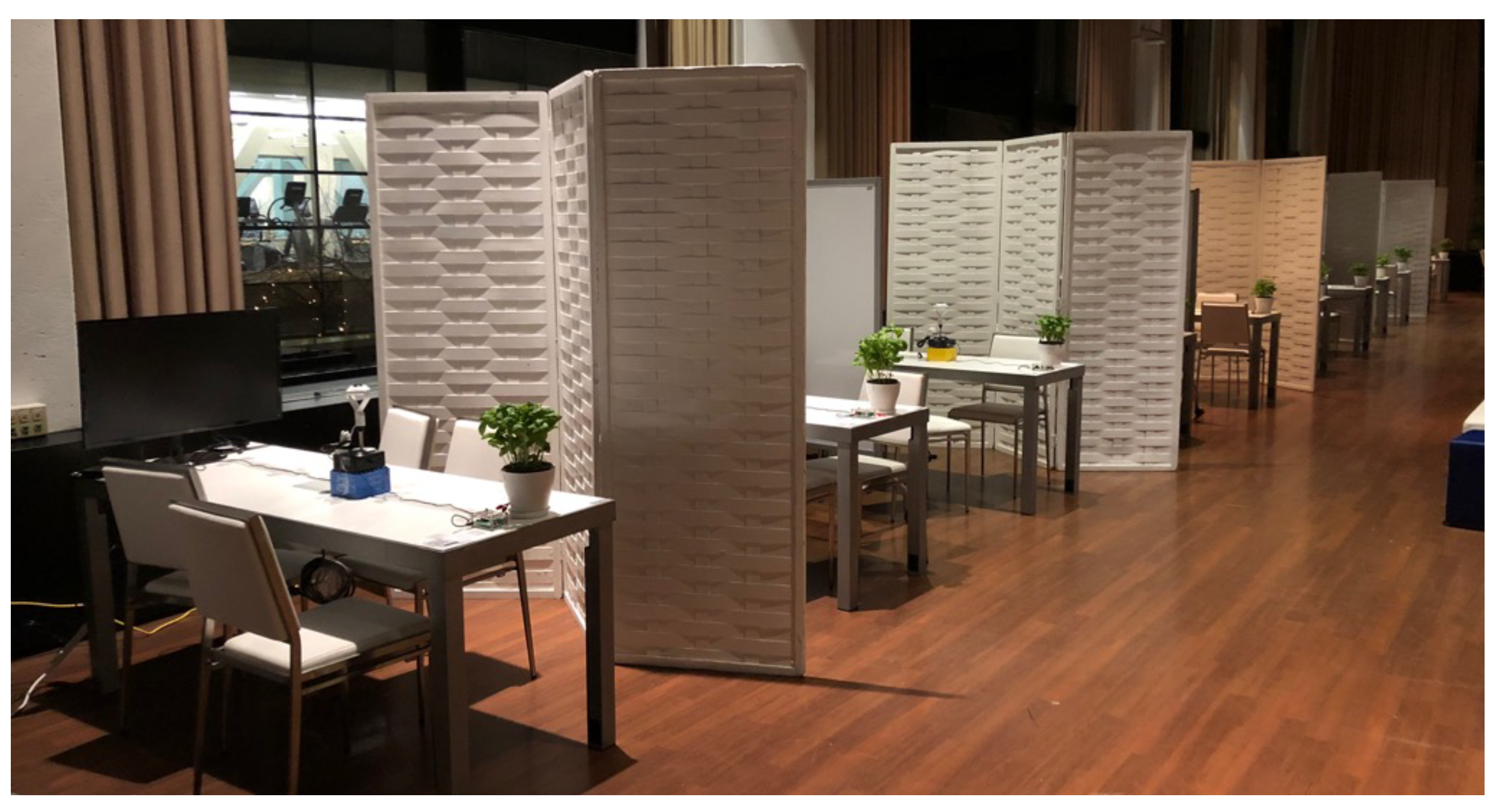
3.1. Teamwork Setting
3.1.1. Study Context
3.1.2. Teams
3.2. Data Collection
3.2.1. Recording
3.2.2. Surveys
3.3. Data Preparation
3.3.1. Data Preprocessing
3.3.2. Speaker Diarization
Face Detection
Face Tracking
Face Cropping
Active Speaker Detection
Scores-to-Speech Segment Transformation
Face-Track Clustering
RTTM File
3.3.3. Audio Feature Calculation
3.3.4. Qualitative Assessment of the Software
Audiovisual Speaker Diarization Evaluation
Audio Feature Calculation Evaluation
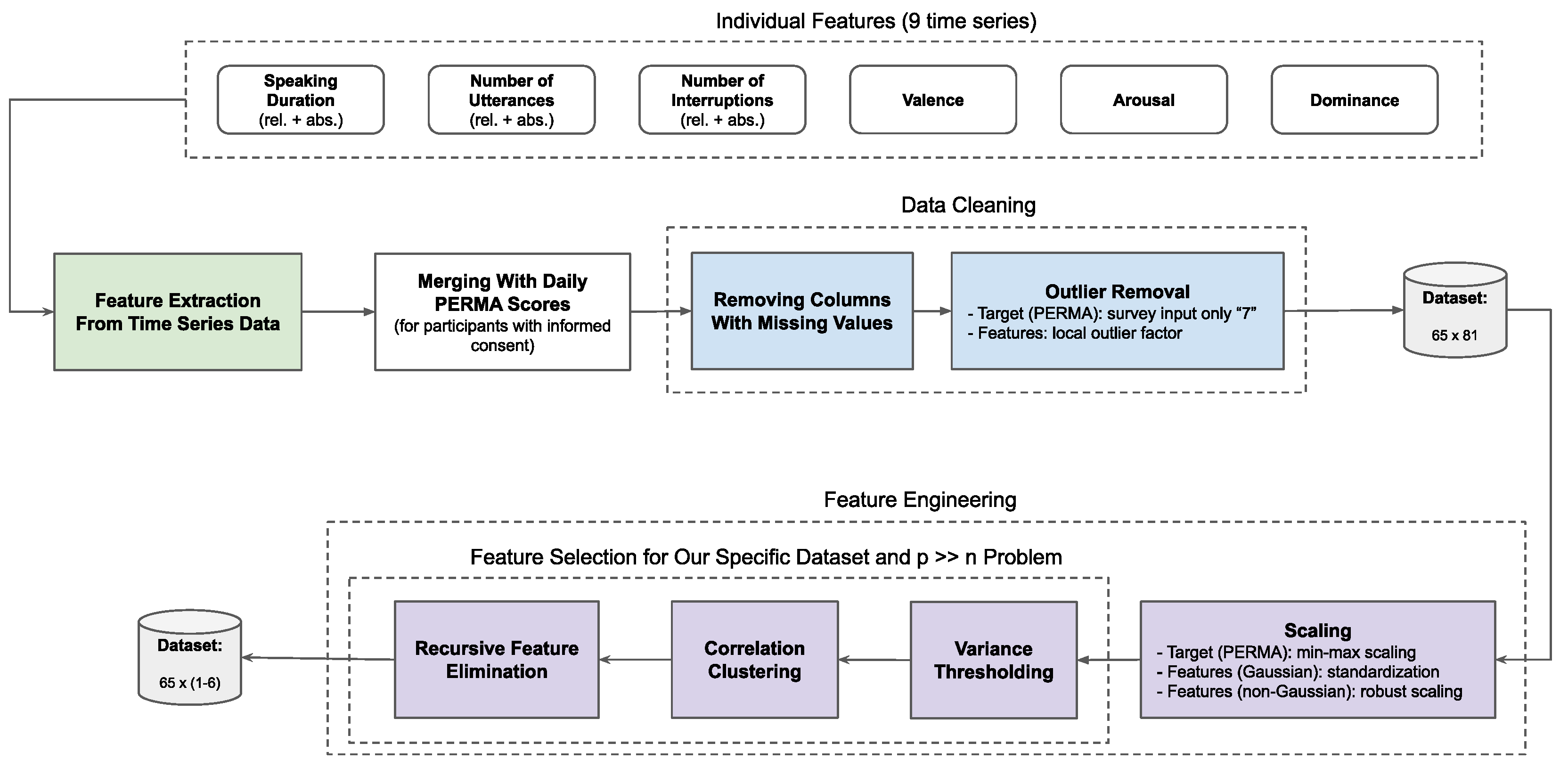
3.3.5. Feature Extraction, Data Cleaning, and Feature Engineering
Feature Extraction from Time Series Data
Outlier Removal
Scaling
Feature Selection
3.4. Data Analysis
3.4.1. Correlation of Features with PERMA Pillars
3.4.2. Evaluation of Classification Models
3.4.3. Feature Importance of Classification Models
4. Results
4.1. Selected Features for Classification Models
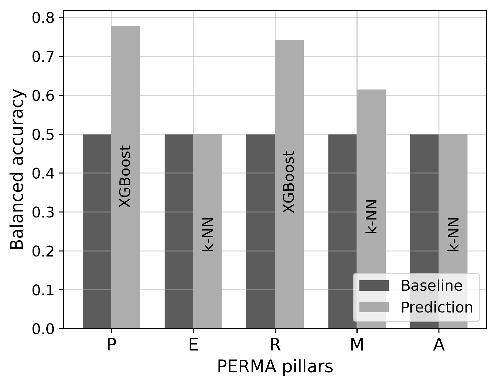
4.2. Evaluation of Classification Models
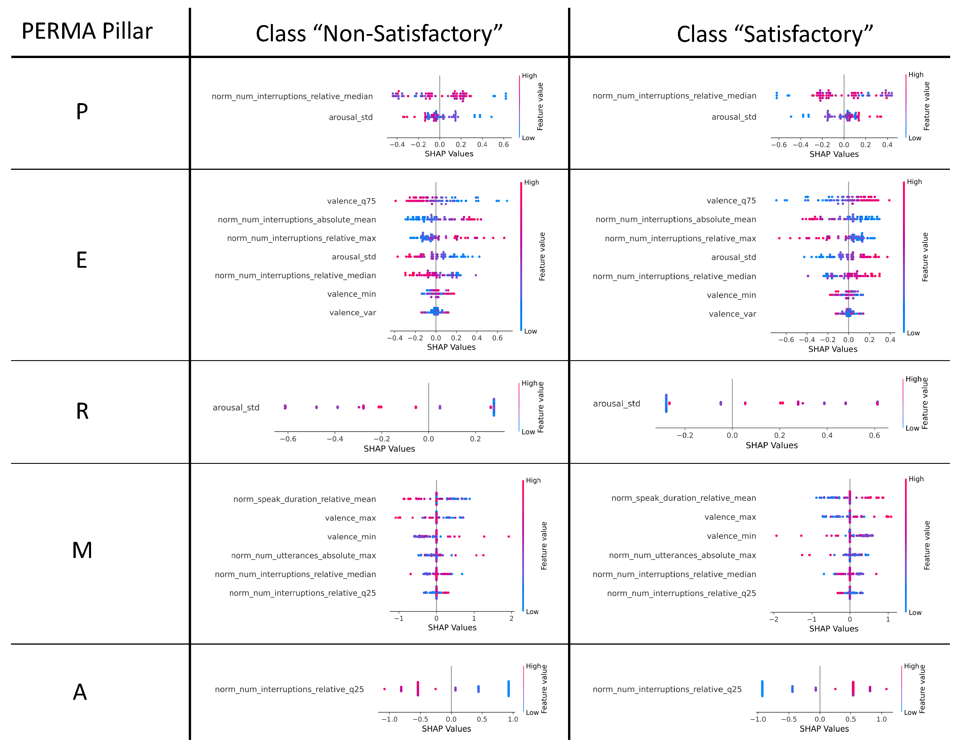
4.3. SHAP Values of Classification Models
5. Findings
5.1. Answers to Research Questions
- RQ1. What are the challenges of individual well-being prediction in team collaboration based on multi-modal speech data? How can they be addressed?
- RQ2. Based on our own data, what algorithms and target labels are suitable for predicting well-being in teamwork contexts based on multi-modal speech data?
- RQ3. Based on our own data, which speech features serve as predictors of individual well-being in team collaboration?
5.2. Limitations
6. Future Work
7. Conclusions
Author Contributions
Funding
Institutional Review Board Statement
Informed Consent Statement
Data Availability Statement
Acknowledgments
Conflicts of Interest
Abbreviations
| AIA | Anonymous Institute |
| AS | Anonymous Study |
| ASD | active speaker detection |
| CatBoost | categorical boosting |
| DBSCAN | density-based spatial clustering of applications with noise |
| fps | frames per second |
| IOU | intersection over union |
| IPO | input-process-output |
| k-NN | k-nearest neighbor |
| LOF | local outlier factor |
| LOOCV | leave-one-out cross-validation |
| MAE | mean absolute error |
| PERMA | positive emotion, engagement, relationships, meaning, and accomplishment |
| RFE | recursive feature elimination |
| RTTM | rich transcription time marked |
| S3FD | single shot scale-invariant face detector |
| SHAP | Shapley additive explanations |
| VER | voice emotion recognition |
| XGBoost | extreme gradient boosting |
Appendix A

References
- World Health Organization. International Classification of Diseases (ICD); World Health Organization: Geneva, Switzerland, 2019. [Google Scholar]
- Gloor, P.A. Happimetrics: Leveraging AI to Untangle the Surprising Link between Ethics, Happiness and Business Success; Edward Elgar Publishing: Cheltenham, UK, 2022. [Google Scholar]
- Landy, F.J.; Conte, J.M. Work in the 21st Century: An Introduction to Industrial and Organizational Psychology; John Wiley & Sons: Hoboken, NJ, USA, 2010. [Google Scholar]
- Seligman, M.E.P. Flourish: A Visionary New Understanding of Happiness and Well-Being; Simon and Schuster: New York, NY, USA, 2012. [Google Scholar]
- Ringeval, F.; Sonderegger, A.; Sauer, J.; Lalanne, D. Introducing the RECOLA multimodal corpus of remote collaborative and affective interactions. In Proceedings of the 2013 10th IEEE International Conference and Workshops on Automatic Face and Gesture Recognition (FG), Shanghai, China, 22–26 April 2013; pp. 1–8. [Google Scholar] [CrossRef]
- Oxelmark, L.; Nordahl Amorøe, T.; Carlzon, L.; Rystedt, H. Students’ understanding of teamwork and professional roles after interprofessional simulation—A qualitative analysis. Adv. Simul. 2017, 2, 8. [Google Scholar] [CrossRef] [PubMed]
- Koutsombogera, M.; Vogel, C. Modeling collaborative multimodal behavior in group dialogues: The MULTISIMO corpus. In Proceedings of the Eleventh International Conference on Language Resources and Evaluation (LREC 2018), Miyazaki, Japan, 7–12 May 2018; European Language Resources Association (ELRA): Luxemburg, 2018. [Google Scholar]
- Sanchez-Cortes, D.; Aran, O.; Jayagopi, D.B.; Schmid Mast, M.; Gatica-Perez, D. Emergent leaders through looking and speaking: From audio-visual data to multimodal recognition. J. Multimodal User Interfaces 2013, 7, 39–53. [Google Scholar] [CrossRef]
- Braley, M.; Murray, G. The group affect and performance (GAP) corpus. In Proceedings of the GIFT’18: Proceedings of the Group Interaction Frontiers in Technology, Boulder, CO, USA, 16 October 2018; Association for Computing Machinery: New York, NY, USA, 2018; pp. 1–9. [Google Scholar] [CrossRef]
- Christensen, B.T.; Abildgaard, S.J.J. Inside the DTRS11 dataset: Background, content, and methodological choices. In Analysing Design Thinking: Studies of Cross-Cultural Co-Creation; CRC Press: Boca Raton, FL, USA, 2017; pp. 19–37. [Google Scholar]
- Ivarsson, J.; Åberg, M. Role of requests and communication breakdowns in the coordination of teamwork: A video-based observational study of hybrid operating rooms. BMJ Open 2020, 10, e035194. [Google Scholar] [CrossRef] [PubMed]
- Brophy, J. (Ed.) Using Video in Teacher Education; Emerald Group Publishing Limited: Bingley, UK, 2003. [Google Scholar]
- Baecher, L.; Kung, S.C.; Ward, S.L.; Kern, K. Facilitating video analysis for teacher development: A systematic review of the research. J. Technol. Teach. Educ. 2018, 26, 185–216. [Google Scholar]
- Kang, W.; Roy, B.C.; Chow, W. Multimodal Speaker diarization of real-world meetings using D-vectors with spatial features. In Proceedings of the ICASSP 2020—2020 IEEE International Conference on Acoustics, Speech and Signal Processing (ICASSP), Barcelona, Spain, 4–8 May 2020; pp. 6509–6513, ISSN 2379-190X. [Google Scholar] [CrossRef]
- Zheng, N.; Li, N.; Wu, X.; Meng, L.; Kang, J.; Wu, H.; Weng, C.; Su, D.; Meng, H. The CUHK-Tencent Speaker Diarization System for the ICASSP 2022 Multi-channel multi-party meeting transcription challenge. In Proceedings of the ICASSP 2022—2022 IEEE International Conference on Acoustics, Speech and Signal Processing (ICASSP), Singapore, Singapore, 23–27 May 2022; pp. 9161–9165, ISSN 2379-190X. [Google Scholar] [CrossRef]
- Hershey, J.R.; Chen, Z.; Roux, J.L.; Watanabe, S. Deep clustering: Discriminative embeddings for segmentation and separation. In Proceedings of the 2016 IEEE International Conference on Acoustics, Speech and Signal Processing (ICASSP), Shanghai, China, 20–25 March 2016. [Google Scholar] [CrossRef]
- Kolbæk, M.; Yu, D.; Tan, Z.H.; Jensen, J. Multi-talker Speech Separation with Utterance-level Permutation Invariant Training of Deep Recurrent Neural Networks. IEEE/ACM Trans. Audio Speech Lang. Process. 2017, 25, 1901–1913. [Google Scholar] [CrossRef]
- Maciejewski, M.; Sell, G.; Garcia-Perera, L.P.; Watanabe, S.; Khudanpur, S. Building Corpora for Single-Channel Speech Separation Across Multiple Domains. arXiv 2018, arXiv:1811.02641. [Google Scholar] [CrossRef]
- Luo, Y.; Mesgarani, N. Conv-TasNet: Surpassing ideal time-frequency magnitude masking for speech separation. IEEE/ACM Trans. Audio Speech Lang. Process. 2019, 27, 1256–1266. [Google Scholar] [CrossRef]
- Park, T.J.; Kanda, N.; Dimitriadis, D.; Han, K.J.; Watanabe, S.; Narayanan, S. A Review of Speaker Diarization: Recent Advances with Deep Learning. Comput. Speech Lang. 2022, 72, 101317. [Google Scholar] [CrossRef]
- Dov, D.; Talmon, R.; Cohen, I. Audio-visual voice activity detection using diffusion maps. IEEE/ACM Trans. Audio Speech Lang. Process. 2015, 23, 732–745. [Google Scholar] [CrossRef]
- Yoshioka, T.; Abramovski, I.; Aksoylar, C.; Chen, Z.; David, M.; Dimitriadis, D.; Gong, Y.; Gurvich, I.; Huang, X.; Huang, Y.; et al. Advances in Online Audio-Visual Meeting Transcription. In Proceedings of the 2019 IEEE Automatic Speech Recognition and Understanding Workshop (ASRU), Singapore, 14–18 December 2019. [Google Scholar] [CrossRef]
- Nagrani, A.; Chung, J.S.; Zisserman, A. VoxCeleb: A large-scale speaker identification dataset. In Proceedings of the Interspeech 2017, Stockholm, Sweden, 20–24 August 2017; pp. 2616–2620. [Google Scholar] [CrossRef]
- Chung, J.S.; Nagrani, A.; Zisserman, A. VoxCeleb2: Deep Speaker Recognition. In Proceedings of the Interspeech 2018, Hyderabad, India, 2–6 September 2018; pp. 1086–1090. [Google Scholar] [CrossRef]
- Chung, J.S.; Huh, J.; Nagrani, A.; Afouras, T.; Zisserman, A. Spot the conversation: Speaker diarisation in the wild. In Proceedings of the Interspeech 2020, Shanghai, China, 25–29 October 2020; pp. 299–303. [Google Scholar] [CrossRef]
- Xu, E.Z.; Song, Z.; Tsutsui, S.; Feng, C.; Ye, M.; Shou, M.Z. AVA-AVD: Audio-visual Speaker Diarization in the Wild. In Proceedings of the MM ’22: 30th ACM International Conference on Multimedia, Lisboa, Portugal, 10–14 October 2022; Association for Computing Machinery: New York, NY, USA, 2022; pp. 3838–3847. [Google Scholar] [CrossRef]
- Chung, J.S.; Lee, B.J.; Han, I. Who said that? Audio-visual speaker diarisation of real-world meetings. In Proceedings of the Interspeech 2019, Graz, Austria, 15–19 September 2019. [Google Scholar] [CrossRef]
- Sonnentag, S. Dynamics of Well-Being. Annu. Rev. Organ. Psychol. Organ. Behav. 2015, 2, 261–293. [Google Scholar] [CrossRef]
- Anglim, J.; Horwood, S.; Smillie, L.D.; Marrero, R.J.; Wood, J.K. Predicting psychological and subjective well-being from personality: A meta-analysis. Psychol. Bull. 2020, 146, 279–323. [Google Scholar] [CrossRef] [PubMed]
- Dejonckheere, E.; Mestdagh, M.; Houben, M.; Rutten, I.; Sels, L.; Kuppens, P.; Tuerlinckx, F. Complex affect dynamics add limited information to the prediction of psychological well-being. Nat. Hum. Behav. 2019, 3, 478–491. [Google Scholar] [CrossRef] [PubMed]
- Smits, C.H.M.; Deeg, D.J.H.; Bosscher, R.J. Well-Being and Control in Older Persons: The Prediction of Well-Being from Control Measures. Int. J. Aging Hum. Dev. 1995, 40, 237–251. [Google Scholar] [CrossRef]
- Karademas, E.C. Positive and negative aspects of well-being: Common and specific predictors. Personal. Individ. Differ. 2007, 43, 277–287. [Google Scholar] [CrossRef]
- Bharadwaj, L.; Wilkening, E.A. The prediction of perceived well-being. Soc. Indic. Res. 1977, 4, 421–439. [Google Scholar] [CrossRef]
- Ridner, S.L.; Newton, K.S.; Staten, R.R.; Crawford, T.N.; Hall, L.A. Predictors of well-being among college students. J. Am. Coll. Health 2016, 64, 116–124. [Google Scholar] [CrossRef]
- van Mierlo, H.; Rutte, C.G.; Kompier, M.A.J.; Doorewaard, H.A.C.M. Self-Managing Teamwork and Psychological Well-Being: Review of a Multilevel Research Domain. Group Organ. Manag. 2005, 30, 211–235. [Google Scholar] [CrossRef]
- Markova, G.; Perry, J.T. Cohesion and individual well-being of members in self-managed teams. Leadersh. Organ. Dev. J. 2014, 35, 429–441. [Google Scholar] [CrossRef]
- Dawadi, P.N.; Cook, D.J.; Schmitter-Edgecombe, M. Automated Cognitive Health Assessment from Smart Home-Based Behavior Data. IEEE J. Biomed. Health Inform. 2016, 20, 1188–1194. [Google Scholar] [CrossRef]
- Casaccia, S.; Romeo, L.; Calvaresi, A.; Morresi, N.; Monteriù, A.; Frontoni, E.; Scalise, L.; Revel, G.M. Measurement of Users’ Well-Being Through Domotic Sensors and Machine Learning Algorithms. IEEE Sens. J. 2020, 20, 8029–8038. [Google Scholar] [CrossRef]
- Rickard, N.; Arjmand, H.A.; Bakker, D.; Seabrook, E. Development of a Mobile Phone App to Support Self-Monitoring of Emotional Well-Being: A Mental Health Digital Innovation. JMIR Ment. Health 2016, 3, e6202. [Google Scholar] [CrossRef] [PubMed]
- Nosakhare, E.; Picard, R. Toward Assessing and Recommending Combinations of Behaviors for Improving Health and Well-Being. ACM Trans. Comput. Healthc. 2020, 1, 1–29. [Google Scholar] [CrossRef]
- Robles-Granda, P.; Lin, S.; Wu, X.; D’Mello, S.; Martinez, G.J.; Saha, K.; Nies, K.; Mark, G.; Campbell, A.T.; De Choudhury, M.; et al. Jointly predicting job performance, personality, cognitive ability, affect, and well-being. IEEE Comput. Intell. Mag. 2021, 16, 46–61. [Google Scholar] [CrossRef]
- Yu, Z.; Li, X.; Zhao, G. Facial-Video-Based Physiological Signal Measurement: Recent advances and affective applications. IEEE Signal Process. Mag. 2021, 38, 50–58. [Google Scholar] [CrossRef]
- Gong, Y.; Poellabauer, C. Topic modeling based multi-modal depression detection. In Proceedings of the AVEC ’17: 7th Annual Workshop on Audio/Visual Emotion Challenge, Mountain View, CA, USA, 23 October 2017; Association for Computing Machinery: New York, NY, USA, 2017; pp. 69–76. [Google Scholar] [CrossRef]
- Gupta, R.; Malandrakis, N.; Xiao, B.; Guha, T.; Van Segbroeck, M.; Black, M.; Potamianos, A.; Narayanan, S. Multimodal prediction of affective dimensions and depression in human-computer interactions. In Proceedings of the AVEC ’14: 4th International Workshop on Audio/Visual Emotion Challenge, Orlando, FL, USA, 7 November 2014; Association for Computing Machinery: New York, NY, USA, 2014; pp. 33–40. [Google Scholar] [CrossRef]
- Williamson, J.R.; Young, D.; Nierenberg, A.A.; Niemi, J.; Helfer, B.S.; Quatieri, T.F. Tracking depression severity from audio and video based on speech articulatory coordination. Comput. Speech Lang. 2019, 55, 40–56. [Google Scholar] [CrossRef]
- Huang, Y.N.; Zhao, S.; Rivera, M.L.; Hong, J.I.; Kraut, R.E. Predicting well-being using short ecological momentary audio recordings. In Proceedings of the CHI EA ’21: Extended Abstracts of the 2021 CHI Conference on Human Factors in Computing Systems, Yokohama, Japan, 8–13 May 2021; Association for Computing Machinery: New York, NY, USA, 2021; pp. 1–7. [Google Scholar] [CrossRef]
- Kim, S.; Kwon, N.; O’Connell, H. Toward estimating personal well-being using voice. arXiv 2019, arXiv:1910.10082. [Google Scholar] [CrossRef]
- Kuutila, M.; Mäntylä, M.; Claes, M.; Elovainio, M.; Adams, B. Individual differences limit predicting well-being and productivity using software repositories: A longitudinal industrial study. Empir. Softw. Eng. 2021, 26, 88. [Google Scholar] [CrossRef]
- Izumi, K.; Minato, K.; Shiga, K.; Sugio, T.; Hanashiro, S.; Cortright, K.; Kudo, S.; Fujita, T.; Sado, M.; Maeno, T.; et al. Unobtrusive Sensing Technology for Quantifying Stress and Well-Being Using Pulse, Speech, Body Motion, and Electrodermal Data in a Workplace Setting: Study Concept and Design. Front. Psychiatry 2021, 12, 611243. [Google Scholar] [CrossRef] [PubMed]
- MIT. MIT SDM-System Design and Management. Available online: https://sdm.mit.edu/ (accessed on 27 March 2023).
- j5create. 360° All Around Webcam. Available online: https://en.j5create.com/products/jvcu360 (accessed on 27 March 2023).
- Lobe, B.; Morgan, D.; Hoffman, K.A. Qualitative Data Collection in an Era of Social Distancing. Int. J. Qual. Methods 2020, 19, 1609406920937875. [Google Scholar] [CrossRef]
- Donaldson, S.I.; van Zyl, L.E.; Donaldson, S.I. PERMA+4: A Framework for Work-Related Wellbeing, Performance and Positive Organizational Psychology 2.0. Front. Psychol. 2022, 12, 817244. [Google Scholar] [CrossRef]
- Wilson, W.R. Correlates of avowed happiness. Psychol. Bull. 1967, 67, 294–306. [Google Scholar] [CrossRef]
- Raja, F.; Akhtar, D.; Hussain, S. Exploring Perception Of Professionals Regarding Introversion And Extroversion In Relation To Success At Workplace. J. Educ. Sci. 2020, 7, 184–195. [Google Scholar]
- Laney, M.O. The Introvert Advantage: How Quiet People Can Thrive in an Extrovert World; Workman Publishing: New York, NY, USA, 2002; Google-Books-ID: o9yEqgTWR_AC. [Google Scholar]
- Yang, S.; Luo, P.; Loy, C.C.; Tang, X. WIDER FACE: A Face Detection Benchmark. In Proceedings of the 2016 IEEE Conference on Computer Vision and Pattern Recognition (CVPR), Las Vegas, NV, USA, 27–30 June 2016; Available online: http://arxiv.org/abs/1511.06523 [cs] (accessed on 6 March 2024).
- Chung, J.S.; Zisserman, A. Out of time: Automated lip sync in the wild. In Proceedings of the Workshop on Multi-View Lip-Reading, ACCV, Taipei, Taiwan, 20–24 November 2016. [Google Scholar]
- Tao, R.; Pan, Z.; Das, R.K.; Qian, X.; Shou, M.Z.; Li, H. Is someone speaking? Exploring long-term temporal features for audio-visual active speaker detection. In Proceedings of the 29th ACM International Conference on Multimedia, Virtual Event, China, 20–24 October 2021; pp. 3927–3935. [Google Scholar] [CrossRef]
- Ryant, N.; Church, K.; Cieri, C.; Cristia, A.; Du, J.; Ganapathy, S.; Liberman, M. First DIHARD Challenge Evaluation Plan. Tech. Rep. 2018. [Google Scholar] [CrossRef]
- Fu, S.W.; Fan, Y.; Hosseinkashi, Y.; Gupchup, J.; Cutler, R. Improving Meeting Inclusiveness USING speech interruption analysis. In Proceedings of the MM ’22: The 30th ACM International Conference on Multimedia, Lisboa Portugal, 10–14 October 2022; Available online: http://arxiv.org/abs/2304.00658 (accessed on 6 March 2024).
- Wagner, J.; Triantafyllopoulos, A.; Wierstorf, H.; Schmitt, M.; Burkhardt, F.; Eyben, F.; Schuller, B.W. Dawn of the transformer era in speech emotion recognition: Closing the valence gap. IEEE Trans. Pattern Anal. Mach. Intell. 2023, 45, 10745–10759. [Google Scholar] [CrossRef]
- Alisamir, S.; Ringeval, F. On the Evolution of Speech Representations for Affective Computing: A brief history and critical overview. IEEE Signal Process. Mag. 2021, 38, 12–21. [Google Scholar] [CrossRef]
- Christ, M.; Braun, N.; Neuffer, J.; Kempa-Liehr, A.W. Time Series FeatuRe Extraction on basis of Scalable Hypothesis tests (tsfresh—A Python package). Neurocomputing 2018, 307, 72–77. [Google Scholar] [CrossRef]
- Breunig, M.M.; Kriegel, H.P.; Ng, R.T.; Sander, J. LOF: Identifying density-based local outliers. ACM SIGMOD Rec. 2000, 29, 93–104. [Google Scholar] [CrossRef]
- Cheng, Z.; Zou, C.; Dong, J. Outlier detection using isolation forest and local outlier factor. In Proceedings of the RACS ’19: Conference on Research in Adaptive and Convergent Systems, Chongqing, China, 24–27 September 2019; Association for Computing Machinery: New York, NY, USA, 2019; pp. 161–168. [Google Scholar] [CrossRef]
- Zheng, A.; Casari, A. Feature Engineering for Machine Learning: Principles and Techniques for Data Scientists; O’Reilly Media, Inc.: Sebastopol, CA, USA, 2018. [Google Scholar]
- Jain, A.; Nandakumar, K.; Ross, A. Score normalization in multimodal biometric systems. Pattern Recognit. 2005, 38, 2270–2285. [Google Scholar] [CrossRef]
- Pedregosa, F.; Varoquaux, G.; Gramfort, A.; Michel, V.; Thirion, B.; Grisel, O.; Blondel, M.; Prettenhofer, P.; Weiss, R.; Dubourg, V.; et al. Scikit-learn: Machine Learning in Python. J. Mach. Learn. Res. 2011, 12, 2825–2830. [Google Scholar]
- Harrel, F.E. Regression Modeling Strategies: With Applications to Linear Models, Logistic and Ordinal Regression, and Survival Analysis; Springer International Publishing: Berlin/Heidelberg, Germany, 2015. [Google Scholar]
- Kelleher, J.D.; Mac Namee, B.; D’Arcy, A. Fundamentals of Machine Learning for Predictive Data Analytics: Algorithms, Worked Examples, and Case Studies; The MIT Press: Cambridge, MA, USA, 2015. [Google Scholar]
- Disabato, D.J.; Goodman, F.R.; Kashdan, T.B.; Short, J.L.; Jarden, A. Different types of well-being? A cross-cultural examination of hedonic and eudaimonic well-being. Psychol. Assess. 2016, 28, 471–482. [Google Scholar] [CrossRef]
- Mirehie, M.; Gibson, H. Empirical testing of destination attribute preferences of women snow-sport tourists along a trajectory of participation. Tour. Recreat. Res. 2020, 45, 526–538. [Google Scholar] [CrossRef]
- Mirehie, M.; Gibson, H. Women’s participation in snow-sports and sense of well-being: A positive psychology approach. J. Leis. Res. 2020, 51, 397–415. [Google Scholar] [CrossRef]
- Giri, V.N. Culture and Communication Style. Rev. Commun. 2006, 6, 124–130. [Google Scholar] [CrossRef]
- Stolcke, A.; Yoshioka, T. DOVER: A method for combining diarization outputs. In Proceedings of the 2019 IEEE Automatic Speech Recognition and Understanding Workshop (ASRU), Singapore, 14–18 December 2019; IEEE: Piscataway, NJ, USA, 2022. [Google Scholar] [CrossRef]
- Rajasekar, G.P.; de Melo, W.C.; Ullah, N.; Aslam, H.; Zeeshan, O.; Denorme, T.; Pedersoli, M.; Koerich, A.; Bacon, S.; Cardinal, P.; et al. A Joint Cross-Attention Model for Audio-Visual Fusion in Dimensional Emotion Recognition. arXiv 2022, arXiv:2203.14779. [Google Scholar] [CrossRef]
- Lee, C.C.; Sridhar, K.; Li, J.L.; Lin, W.C.; Su, B.; Busso, C. Deep Representation Learning for Affective Speech Signal Analysis and Processing: Preventing unwanted signal disparities. IEEE Signal Process. Mag. 2021, 38, 22–38. [Google Scholar] [CrossRef]
- Müller, M. Predicting Well-Being in Team Collaboration from Video Data Using Machine and Deep Learning; Technical University of Munich: Munich, Germany, 2023; in press. [Google Scholar]
- Radford, A.; Kim, J.W.; Xu, T.; Brockman, G.; McLeavey, C.; Sutskever, I. Robust Speech Recognition via Large-Scale Weak Supervision. arXiv 2023, arXiv:2212.04356. [Google Scholar] [CrossRef]


| Pillar | # Features | Selected Feature(s) |
|---|---|---|
| P | 2 | norm_num_interruptions_relative_median, arousal_std |
| E | 7 | valence_min, valence_q75, norm_num_interruptions_relative_median, arousal_std, valence_var, norm_num_interruptions_absolute_mean, norm_num_interruptions_relative_max |
| R | 1 | arousal_std |
| M | 6 | valence_min, valence_max, norm_num_interruptions_relative_median, norm_speak_duration _relative_mean, norm_num_interruptions_relative_q25, norm_num_utterances_absolute_max |
| A | 1 | norm_num_interruptions_relative_q25 |
| Classifier | Hyperparameters |
|---|---|
| k-NN | n_neighbors: [3, 5, 7, 9, 11, 13, 15], weights: [‘uniform’, ‘distance’], metric: [‘euclidean’, ’manhattan’] |
| Random forests | n_estimators: [100, 200], max_depth: [3, 5, 7] |
| XGBoost | learning_rate: [0.01, 0.1], max_depth: [3, 5, 7] |
| CatBoost | learning_rate: [0.01, 0.1], depth: [3, 5, 7] |
Disclaimer/Publisher’s Note: The statements, opinions and data contained in all publications are solely those of the individual author(s) and contributor(s) and not of MDPI and/or the editor(s). MDPI and/or the editor(s) disclaim responsibility for any injury to people or property resulting from any ideas, methods, instructions or products referred to in the content. |
© 2024 by the authors. Licensee MDPI, Basel, Switzerland. This article is an open access article distributed under the terms and conditions of the Creative Commons Attribution (CC BY) license (https://creativecommons.org/licenses/by/4.0/).
Share and Cite
Zeulner, T.; Hagerer, G.J.; Müller, M.; Vazquez, I.; Gloor, P.A. Predicting Individual Well-Being in Teamwork Contexts Based on Speech Features. Information 2024, 15, 217. https://doi.org/10.3390/info15040217
Zeulner T, Hagerer GJ, Müller M, Vazquez I, Gloor PA. Predicting Individual Well-Being in Teamwork Contexts Based on Speech Features. Information. 2024; 15(4):217. https://doi.org/10.3390/info15040217
Chicago/Turabian StyleZeulner, Tobias, Gerhard Johann Hagerer, Moritz Müller, Ignacio Vazquez, and Peter A. Gloor. 2024. "Predicting Individual Well-Being in Teamwork Contexts Based on Speech Features" Information 15, no. 4: 217. https://doi.org/10.3390/info15040217
APA StyleZeulner, T., Hagerer, G. J., Müller, M., Vazquez, I., & Gloor, P. A. (2024). Predicting Individual Well-Being in Teamwork Contexts Based on Speech Features. Information, 15(4), 217. https://doi.org/10.3390/info15040217