Time Series Forecasting with Missing Data Using Generative Adversarial Networks and Bayesian Inference

Abstract

This paper tackles the challenge of time series forecasting in the presence of missing data. Traditional methods often struggle with such data, which leads to inaccurate predictions. We propose a novel framework that combines the strengths of Generative Adversarial Networks (GANs) and Bayesian inference. The framework utilizes a Conditional GAN (C-GAN) to realistically impute missing values in the time series data. Subsequently, Bayesian inference is employed to quantify the uncertainty associated with the forecasts due to the missing data. This combined approach improves the robustness and reliability of forecasting compared to traditional methods. The effectiveness of our proposed method is evaluated on a real-world dataset of air pollution data from Mexico City. The results demonstrate the framework’s capability to handle missing data and achieve improved forecasting accuracy.

1. Introduction

Time series forecasting plays a crucial role in various domains from finance and weather prediction to inventory management and anomaly detection. It involves uncovering patterns and trends in historical data to predict future values over time. However, the accuracy of these predictions hinges on several critical factors:

• Data Quality: High-quality data, free from errors and inconsistencies, is essential for reliable forecasts.
• Method Selection: The choice of an appropriate forecasting method hinges on the characteristics of the time series data. For instance, stationary data are often well-suited for ARIMA (Autoregressive Integrated Moving Average) models. In contrast, non-stationary data may necessitate more advanced techniques. Additionally, nonlinear neural network models can be effective for complex time series.
• Incorporation of External Factors: Often, relevant external factors, like weather patterns or economic trends, can significantly influence future values. Including these factors in the forecasting model can improve its accuracy.

A particularly significant challenge in time series forecasting is the presence of missing data. Missing data points disrupt the underlying patterns and can severely impact both data quality and model selection. Traditional statistical methods, such as ARIMA models, are often limited by their linear nature, leading to lower accuracy when dealing with complex relationships and missing values.

To address these limitations, various approaches have been developed, which are categorized as statistical and physical methods. Ref. [1] proposed a novel method for ultra-short-term wind power prediction combining nonlinear data analysis, decomposition, and machine learning. Statistical methods, like interpolation or moving averages, are generally suited for short-term forecasting. Conversely, physical methods, based on domain knowledge, are often used for long-term forecasting. However, each approach has its own limitations and may not be universally applicable.

Neural networks (NNs) have become a prevalent choice for modeling time series data. Ref. [2] reviewed various neural network techniques used for time series prediction tasks. Their key strength lies in their ability to represent complex or dynamic relationships using relatively simple architectures. Unlike traditional statistical methods, neural networks do not require prior assumptions about the underlying statistical properties of the data. Ref. [3] used a neural network to forecast daily average PM10 concentrations in Belgium. This makes them well suited for problems where the data distribution is unknown or non-standard.

The detrimental effect of missing data on forecasting accuracy has been extensively documented. Ref. [4] addressed time series forecasting with missing data using a combination of neural networks and meta-transfer learning. Techniques like transfer learning and ensemble learning have demonstrated promise in mitigating this issue. Ref. [5] introduced a domain adaptation approach for neural networks to compensate for drift in electronic nose systems. Transfer learning leverages knowledge gained from similar datasets to improve performance on the target data with missing values. Ensemble learning combines predictions from multiple models to potentially yield more robust results. However, there is still a need for more effective methods that can comprehensively address the complexities of missing data in time series forecasting. Ref. [6] presented a novel framework for applying transfer learning to time series forecasting problems.

Generative Adversarial Networks (GANs) have emerged as a powerful tool in various data science applications. Ref. [7] discussed Generative Adversarial Networks (GANs) in the context of neural networks. These deep learning models are adept at generating realistic and synthetic data. Notably, Conditional Generative Adversarial Networks (C-GANs) allow for generating data conditioned on specific features, making them particularly well suited for the task of imputing missing values in time series data. Ref. [8] explored image-to-image translation using conditional adversarial networks. By training a C-GAN on complete time series examples, the model can learn the underlying data distribution and generate realistic values to fill in the missing gaps. Ref. [9] proposed a conditional LSTM-GAN architecture for melody generation based on lyrics.

Bayesian inference offers a complementary approach by providing a framework for quantifying the uncertainty associated with forecasts, especially when dealing with missing data. Ref. [10] introduced a probabilistic inference-based least squares support vector machine for noisy environments. This uncertainty quantification is crucial because missing data inherently introduce an element of doubt in the predicted values. Ref. [11] explored neural networks for probability prediction, including applications in nuclear stability and decay. By integrating Bayesian inference with a GAN-based imputation approach, the realistic missing value replacements can not only be generated, but the level of confidence is also estimateed.

While there have been attempts to merge neural networks with Bayesian approaches, these efforts have not fully exploited the strengths of both techniques. Existing methods include using neural networks for tasks like distribution identification with statistical backpropagation [12], probability distribution recognition, and sampling with Monte Carlo or Markov chains. Ref. [11] provided a general overview of neural networks. Ref. [10] discussed deep learning for sampling from various probability distributions. However, the computational complexity of calculating conditional probabilities often necessitates numerical methods like Markov Chain Monte Carlo (MCMC) to determine posterior distributions. In contrast, our proposed approach leverages the unique advantages of both neural networks and Bayesian inference. At each step, Bayesian inference utilizes the newly arrived data as the prior distribution and the neural network’s output as the likelihood. This allows us to obtain the posterior distribution and subsequently update the prior distribution with the new data for the next iteration.

In this paper, a novel time series forecasting framework is proposed that leverages the strengths of both GANs and Bayesian inference. The framework utilizes a C-GAN architecture to impute missing values in the time series data. Following imputation, Bayesian inference is integrated to quantify the uncertainty associated with the forecasts. This combined approach allows for more robust and reliable forecasting in the presence of missing data. The effectiveness of proposed method is evaluated on a real-world dataset of air pollution data from Mexico City. This application demonstrates the framework’s capability to handle missing data and improve forecasting accuracy in a practical scenario.

2. Time Series Forecasting with Missing Data Using Neural Networks

This paper explores the application of neural networks for time series forecasting particularly when dealing with missing data. While ARIMA models are commonly used for non-stationary time series (like air pollution prediction), their performance can deteriorate with missing data, noise, or limited samples. Neural networks offer a more robust alternative for such scenarios; see Figure 1.

2.1. Neural Networks for Time Series Forecasting

The prediction of a time series is presented with $\left\{x_i\right\}$, $i=1\cdots N.$ At time k, the NARMAX model [13] can be used to predict the m-step ahead value $x_{k+m}$ as

$$x_{k+m}=\mathrm{\Phi }(x_k,x_{k-1},\dots ,x_{k-n})$$

(1)

where $\mathrm{\Phi }$ is an unknown nonlinear function, n is the best regression times, or

$$x_{k+m}=\mathrm{\Phi }\left[X_k\right]$$

(2)

where $X_k=[x_k,x_{k-1},\dots ,x_{k-N+1}]$. A neural network to predict $x_{k+m}$ can be expressed as

$${\widehat{x}}_{k+m}=NN[(x_k,x_{k-1},\dots ,x_{k-n})]$$

(3)

where ${\widehat{x}}_{k+m}$ is the output of the neural network, n is the approximation regression times, and $k=1,\cdots ,N$, $NN\left(·\right)$ is the neural network.

For a single-layer neural network, the neural model $NN\left(·\right)$ in (3) is

$${\widehat{x}}_{k+m}=\varphi \left[W_k{\widehat{X}}_k\right]$$

(4)

where $W_k\in R^n$ is the weight matrix, $\varphi$ is the activation function, and ${\widehat{X}}_k=[x_k,x_{k-1},\dots ,x_{k-n}].$

For multilayer neural networks,

$${\widehat{x}}_{k+m}=V_k\varphi \left[W_k{\widehat{X}}_k\right]$$

(5)

where the weight of the hidden layer $W_k\in R^{m\times n}$, and the weight of the output layer $V_k\in R.$

For a deep neural network

$${\widehat{x}}_{k+m}=V_k\varphi \left\{W_1{\varphi }_1\left[\cdots W_l{\widehat{X}}_k\right]\right\}$$

(6)

where l is the number of hidden layers.

The proposed method is out-of-sample prediction: This refers to using new, unseen data to test how well the model performs on data which it has not encountered before. (1) The data are split into two sets: a training set and a testing set. (2) The model is trained on the training set. (3) The trained model is used to make predictions on the testing set (data it has not seen before). (4) The predictions are compared to the actual values in the testing set to assess the model’s accuracy on unseen data.

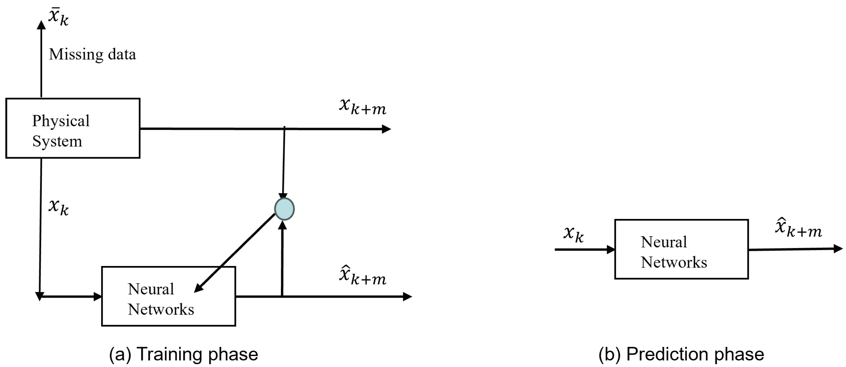
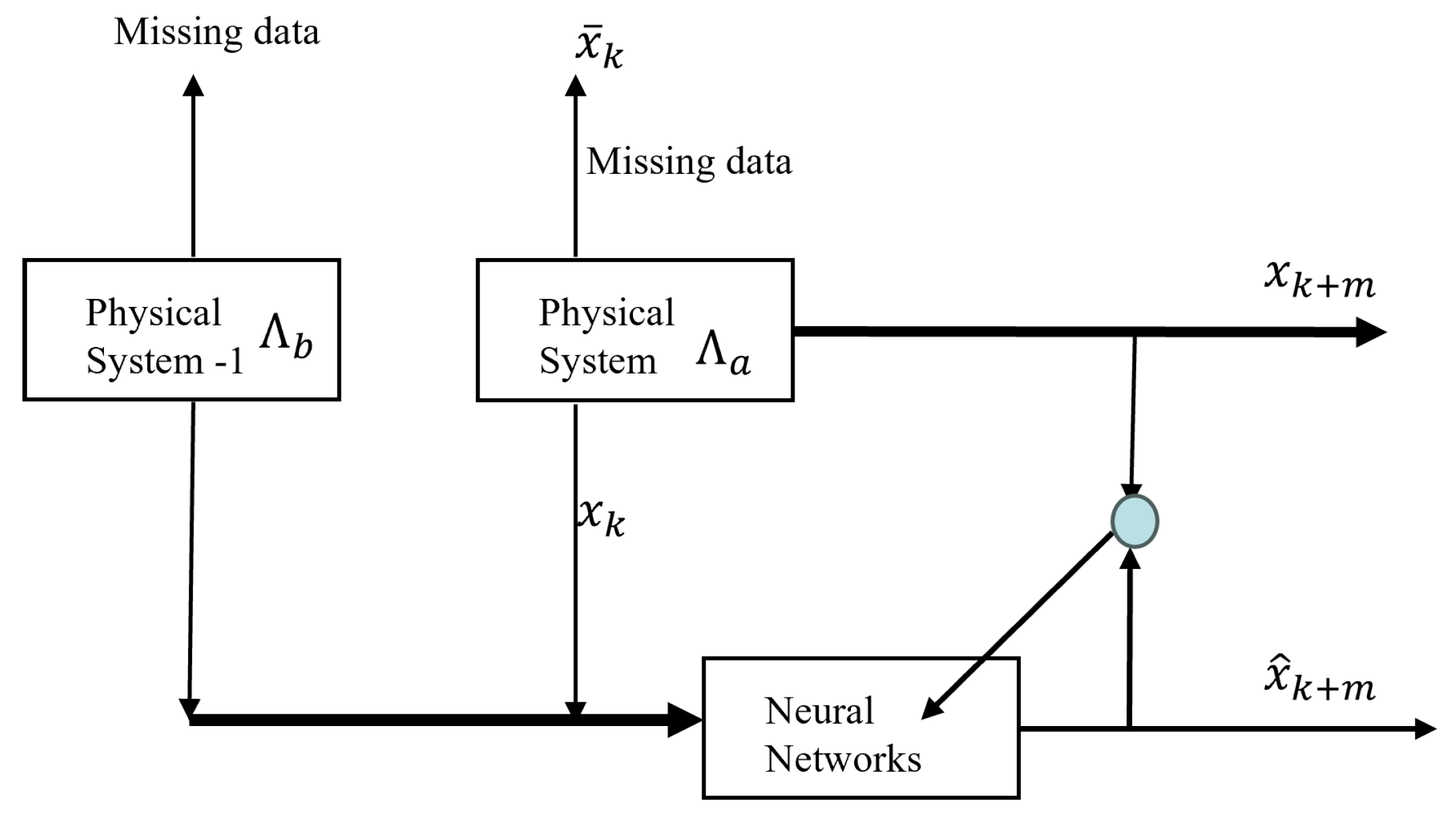
2.2. Neural Networks Training with Missing Data

Traditional neural network training requires large amounts of data and struggles with uncertainties like missing values. To address this challenge, transfer learning is utilized. This technique uses pre-trained models on similar data to improve learning when dealing with limited datasets.

In this paper, the datasets from similar domains (denoted as ${\mathrm{\Lambda }}_a$ and ${\mathrm{\Lambda }}_b$) are used to compensate for missing information in the target domain (${\mathrm{\Lambda }}_a$). Formally, ${\mathrm{\Lambda }}_a$ and ${\mathrm{\Lambda }}_b$ represent matrices of past observations:

$$\begin{array}{c}{\mathrm{\Lambda }}_a=X^a=[x_k^a,x_{k-1}^a,\dots ,x_{k-n}^a]\\ {\mathrm{\Lambda }}_b=X^b=[x_k^b,x_{k-1}^b,\dots ,x_{k-n}^b]\end{array}$$

(7)

${\mathrm{\Lambda }}_a$ and ${\mathrm{\Lambda }}_b$ belong to similar domains because they share similar geographical conditions, such as position and physical characteristics.

These matrices capture the temporal dynamics of each domain. By exploiting the inherent relationships between these domains, the knowledge from ${\mathrm{\Lambda }}_b$ is extracted to fill the gaps in ${\mathrm{\Lambda }}_a$; see Figure 2.

Two strategies can be employed:

• Joint Training: Train model $M_a$ directly using both datasets {${\mathrm{\Lambda }}_a$,${\mathrm{\Lambda }}_b$}.
• Pre-training and Fine-tuning: Pre-train $M_a$ with the complete data ${\mathrm{\Lambda }}_b$; then, fine-tune it with the target data ${\mathrm{\Lambda }}_a$.

The success of this approach hinges on effectively transferring features from the information-rich domain (${\mathrm{\Lambda }}_b$) to the data-scarce target domain (${\mathrm{\Lambda }}_a$).

The objective of the neural network modeling is to minimize the modeling error defined as shown below:

$$e_k={\widehat{x}}_{k+m}-x_{k+m}$$

(8)

The updating law for the weights $W_k$ and $V_k$ is obtained by

$$NN\left(·\right)=arg\underset{W_k,V_k}{min}\left\{\frac{1}{2N}\sum _{k=1}^N{e}_k^2\right\}$$

(9)

This is achieved by updating the weights

$$W_{k+1}=W_k-\eta \frac{\partial J}{\partial W},V_{k+1}=V_k-\eta \frac{\partial J}{\partial V}$$

(10)

The following gradient method can minimize (9),

$$\begin{array}{c}{W}_{k+1}=W_k-\eta \frac{\partial J}{\partial W}+\alpha \Delta W_k\hfill \\ V_{k+1}=V_k-\eta \frac{\partial J}{\partial V}+\alpha \Delta V_k\hfill \end{array}$$

(11)

where $\Delta W_k=W_k-W_{k-1}$ and $\alpha$ is the positive constant, $0<\eta <1.$

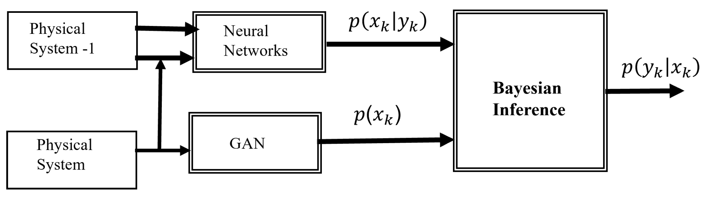
3. Addressing Missing Data in Time Series Forecasting with Generative Adverserial Networks (GANs) and Bayesian Inference

While neural networks are powerful tools for time series forecasting, their training requires large amounts of complete data. When dealing with time series containing missing values, directly applying them can hinder performance. This section proposes a two-step approach to address this challenge.

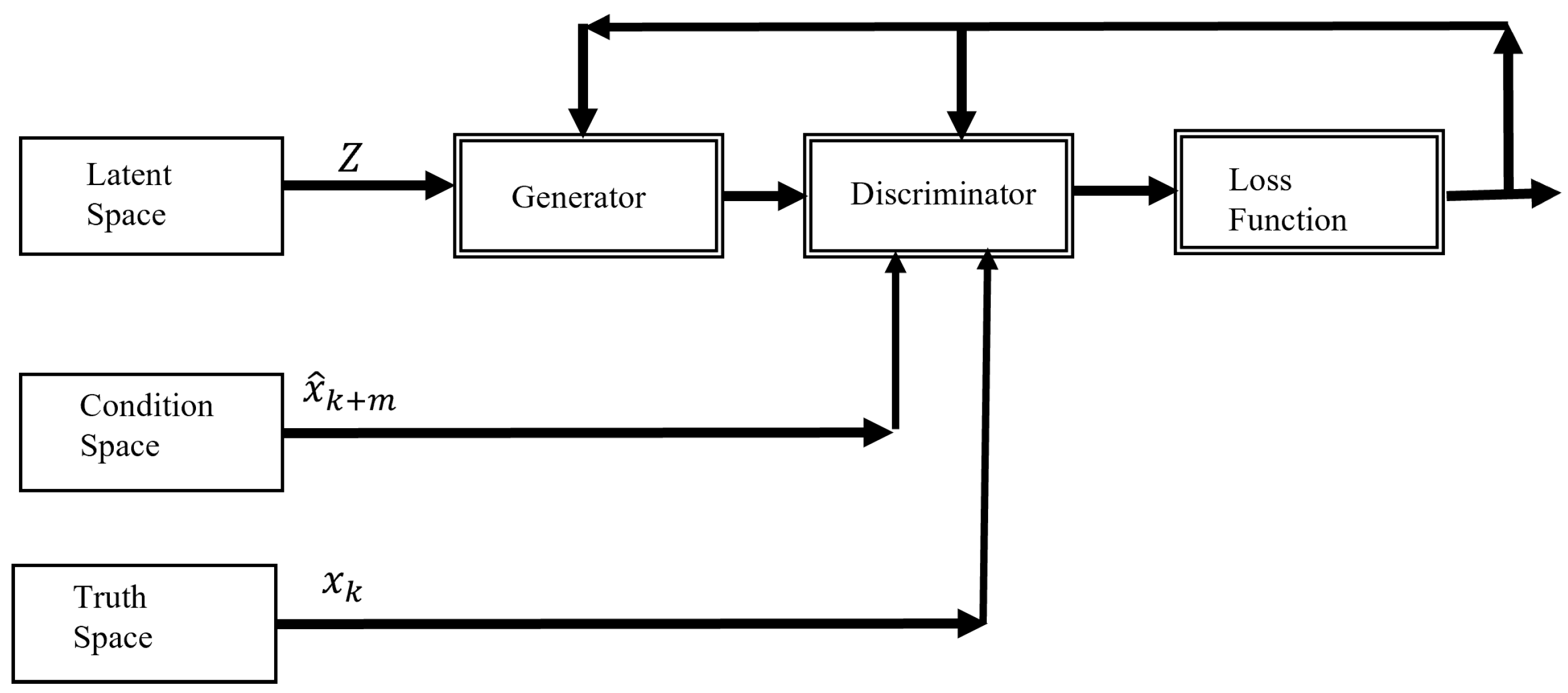
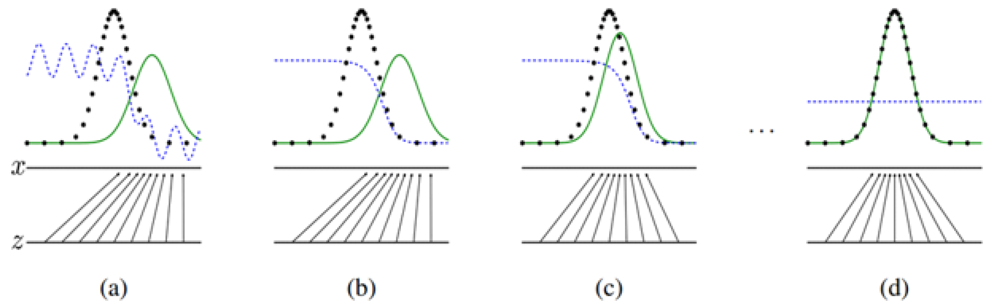
3.1. Learning the Underlying Distribution with Conditional GANs

A time series to be considered as

$$y=\left\{x_i,{\overline{x}}_j\right\}$$

where $x_i$ ($i=1\cdots N$) represent observed data points, and ${\overline{x}}_j$ ($j=1\cdots M$) represent missing values.

To learn the underlying distribution $p\left(x_i\right)$ of the real time series $x_i$ (even with limited data), a Conditional Generative Adversarial Network (C-GAN) is employed.

A C-GAN is a type of neural network architecture involved in a two-player game. One player, the generator, attempts to create samples that statistically resemble the training data. The other player, the discriminator, aims to distinguish between real data and the generator’s creations. Through this competition, the generator progressively learns to produce realistic samples; see Figure 3.

In our case, the C-GAN utilizes information from the observed data points $x_i$. This allows it to capture the relationships within the time series and generate data points that are likely to have occurred alongside the observed values.

Here is a breakdown of the C-GAN components:

(1) Latent Space: This space contains random noise, which is used as an input to the generator

$$Z=\left\{z_k\right\},z_k\sim \mathcal{N}(0,1)$$

(12)

where $z_i$ represents components, and $z_i$ represents normally distributed random numbers with normalized amplitude under $Z=\frac{Z}{max\left\{\right|Z\left|\right\}}$.

(2) Conditioning Signal Space: This space incorporates information from the observed data points x, influencing the type of data the generator creates.

(3) Truth Space: This represents the actual distribution of the missing values

$$P_T:E_T\to [0,1],P_T\left(E_T\right)=\int p_{r}d\tau$$

where $p_T$ is the probability distribution of the truth space, $E_T\sim p_T$

(4) Generator: This network takes noise from the latent space and conditioning signals as inputs, and it outputs potential missing data points that align with the observed data.

$$P_G:E_G\to [0,1],P_G\left(E_G\right)=\int p_{G}d\tau$$

(5) Discriminator: This network attempts to differentiate between real missing values ${\overline{x}}_j$ and the generator’s outputs. It helps refine the generator’s ability to produce realistic data.

$$\begin{array}{c}G:Z\times x_k\to {\widehat{x}}_{k+m}\hfill \\ D:Z\times x_k\times x_{k+m}\to 0\hfill \end{array}$$

(13)

By training these components together, the C-GAN learns to generate missing data points that statistically match the observed time series.

The two-player game is represented by Equation (23), in which both players are both differentiable with respect to their inputs and parameters. Each player has a cost function that depends on the parameters of both players. The discriminator aims to minimize $J^D({\theta }^D,{\theta }^G)$ by optimizing over ${\theta }^D$ alone [14]. Conversely, the generator seeks to minimize $J^G({\theta }^D,{\theta }^G)$ by adjusting its own parameters ${\theta }^G$ only. ${\theta }^D\in {\mathrm{\Theta }}^D$ and ${\theta }^G\in {\mathrm{\Theta }}^G$ are defined as the discriminator and generator strategies, respectively. The strategy spaces are denoted by ${\mathrm{\Theta }}^D$ and ${\mathrm{\Theta }}^G$.

The probability distribution function of the generated space is defined as $p_G$, which is a function parameterized by the parameters ${\theta }^G$, $p_G(K_T,{\theta }^G)$. The training goal is to estimate ${\theta }^G$, which can be achieved by maximizing the likelihood between the spaces $K_T$ and $K_G$:

$${\theta }^{G\ast }=\underset{{\theta }^G}{argmax}{\mathbb{E}}_{K_T\sim p_T}log{p}_G(K_T;{\theta }^G),$$

(14)

which can be considered as a minimization of the divergence KL

$${\theta }^{G\ast }=\underset{{\theta }^G}{argmin}{D}_{KL}(p_T\left(K_T\right)\left|\right|p_G(K;{\theta }^G)).$$

(15)

where $D_{KL}$ is the Kullback–Leibler divergence ($KL$ distance), which is defined by

$$KL\left(p\left(a\mid x\right)\Vert p\left(b\mid x\right)\right)=\sum _i^n{p}_i\left(b\mid x\right)log\left(\frac{p_i\left(b\mid x\right)}{p_i\left(a\mid x\right)}\right)$$

(16)

Then, the generator produces $p_G$ with the same probability distribution of $p_T$

$$p_T\left(\right)\to p_G\left({\theta }^G\right)$$

(17)

The player cost functions are

$$J^D,J^G:{\theta }^D\times {\theta }^G\to \mathcal{R}$$

(18)

Then, a local Nash equilibrium $({\theta }^D,{\theta }^G)$ is obained if

$$\frac{\partial J^D}{\partial {\theta }^D}=0,\frac{\partial J^G}{\partial {\theta }^G}=0$$

(19)

and

$$\frac{{\partial }^2{J}^D}{\partial {{\theta }^D}^2}\ge 0,\frac{{\partial }^2{J}^G}{\partial {{\theta }^G}^2}\ge 0$$

(20)

Since the discriminator function can be interpreted as a binary classifier to distinguish between true and false, it is beneficial to use the cross-entropy function for binary classification as the cost function for the discriminator, as suggested by [15]. The cross-entropy function can be defined as follows:

$$\begin{array}{c}{J}^D=E_{\left(T\right)}\left[logD(x_k,x_{k+m};{\theta }^D)\right]\\ +E_{z\sim p_z\left(z\right)}\left[log(1-D\left(G(z,x_k,x_{k+m};{\theta }^G)\right),u,y)\right]\end{array}$$

Then,

$$J^D=E_{p_T}[log\left(p\left(T\right)\right]+E_{z\sim p_z\left(z\right)}[log\left(p\left(G\right)\right]$$

Considering the game as zero sum,

$$J^G+J^D=0$$

(21)

The objective function of the GAN is

$$\underset{G}{min}\underset{D}{max}V(D,G),V(D,G)=J^G=-J^D$$

(22)

Once the GAN has been trained, $p_G$ becomes a mapping from the latent space to the generated gain space, which is conditioned by the response of a dynamic system. Specifically,

$$p_G=G(Z,x_k,x_{k+1},{\theta }^G)$$

(23)

where ${\theta }^G$ is the parameter vector. The learning process of GAN is shown in Figure 4.

3.2. Bayesian Inference for Forecasting

Once the C-GAN is trained, it can generate potential values to fill in the missing data points. However, there might be some uncertainty associated with these generated values. To address this, Bayesian inference is applied; see Figure 5.

Bayesian inference is a statistical method that incorporates prior knowledge or beliefs into the analysis. In this paper, the C-GAN is used to generate data points alongside the observed data to create a probability distribution for the missing values. This distribution reflects not only the generated values but also considers the inherent uncertainty in the data,

$$p\left(y_k\mid x_k\right)=\frac{p\left(x_k\mid y_k\right)p\left(x_k\right)}{\sum p\left(x_k\right)}\propto p\left(x_k\mid y_k\right)p\left(x_k\right)$$

(24)

At the operating point $x_i,$$p\left(y_k\mid x_k\right)$ is the probability property (posterior distributions) of $y_k$ under the probability distribution $x_k.p\left(x_k\right)$ is from the GAN model (prior distribution), and $p\left(x_k\mid y_k\right)$ is the likelihood, which will be modeled by deep neural networks with transfer learning.

The model of the neural network discussed above is used to generate the likelihood $p\left(x_k\mid y_k\right)$. Because

$$p\left(a\mid b\right)=\frac{p\left(b,a\right)}{p\left(b\right)},E\left[b|a\right]=\sum _{x}bp\left(b|a\right)$$

(25)

the neural network modeling in fact is to minimize the likelihood distribution error as

$$L=\prod _{i=1}^{n}p\left({\theta }^i,x_k^i\right)=\prod _{i=1}^{n}p\left({\theta }^i|x_k^i\right)p\left(x_k^i\right)$$

(26)

The objective of calculating $p\left(x_k\mid y_k\right)$ for the neural network is to update the weights value. In order to maximize the likelihood, the logarithm cost function is used,

$$E=-lnL=-\sum _{i=1}^n\sum _{j=1}^{N}lnp\left({\theta }_j^i|x_k^i\right)-\sum _{i=1}^{n}lnp\left(x_k^i\right)$$

(27)

where N is the training data number.

(1) Given $x_k$ and $x_{k+1}$, the structure of the GAN for identification can be implemented as follows:

$${\widehat{x}}_{k+1}=\sigma \left(W_O\left(k\right)\left[X_k\right]\right)tanh\left(x_k\right)$$

(28)

where

$$x_{k+1}=\sigma \left(W_F\left(k\right)\left[X_k\right]\right)x_k)$$

(29)

where $W_F$ and $W_O$ are the weights.

(2) To compensate for the mapping, multilayer perceptrons are used as

$${\widehat{K}}_G=F\left(W\mathrm{\Psi }\right)$$

(30)

where W is the weight matrix and $\mathrm{\Psi }={[X_k,x_{k+1}]}^T$ is the input vector.

By combining the C-GAN’s ability to learn the underlying distribution and Bayesian inference’s capability to handle uncertainty, a more robust approach is created for time series forecasting with missing data.

4. Air Pollution Forecasting

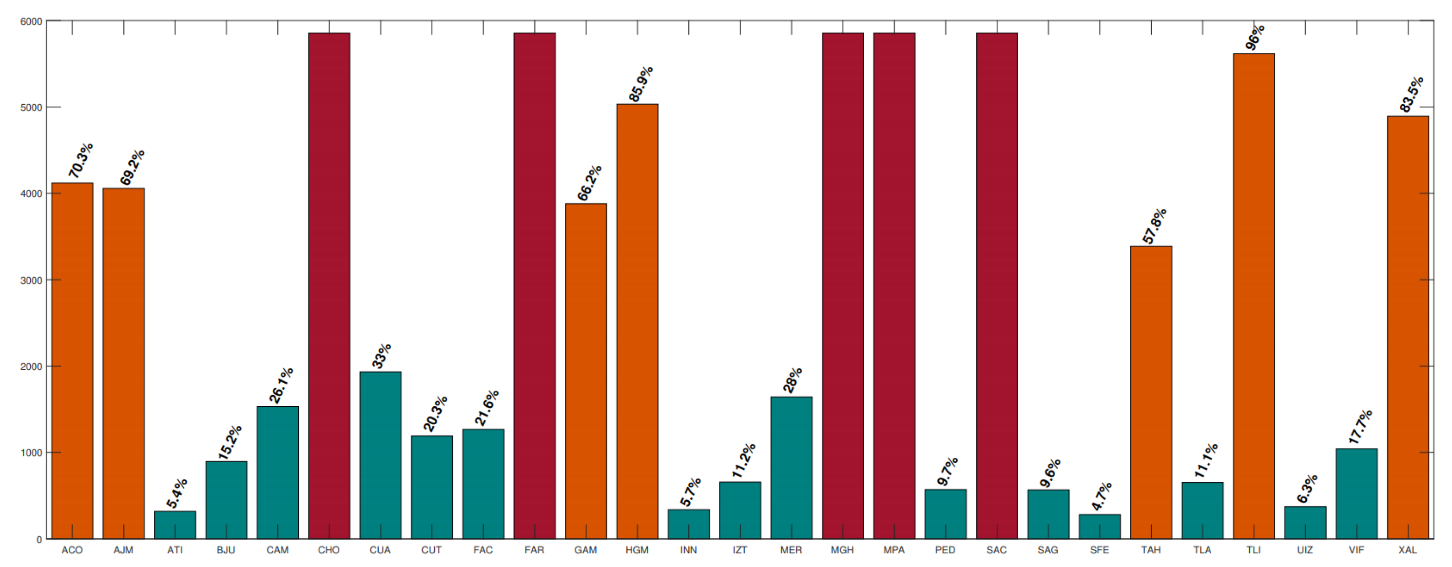
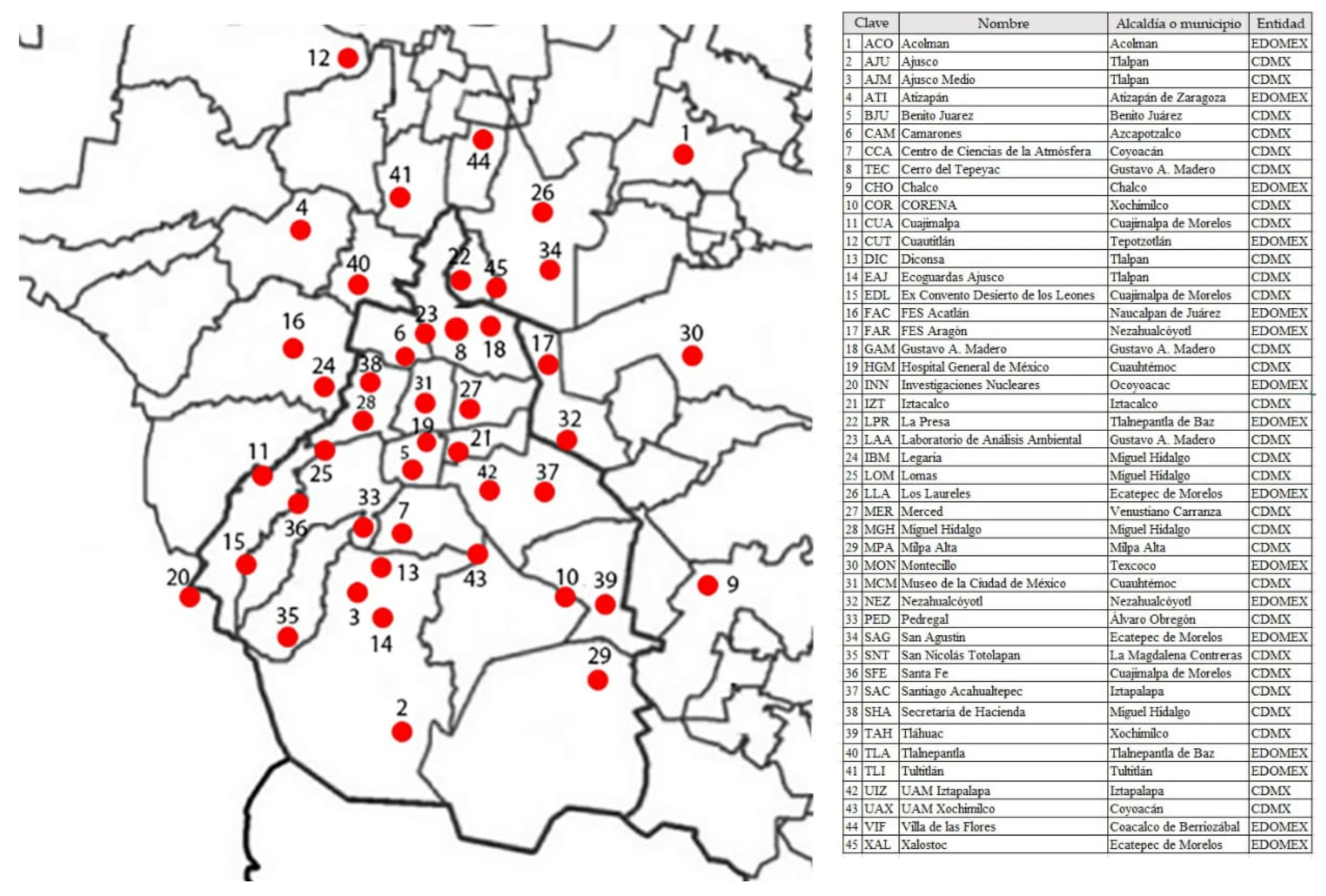
4.1. Air Pollution Data of Mexico City

Mexico City’s environmental monitoring network consists of 43 stations, as shown in Figure 6. As per 2020 data, five stations experienced complete failure throughout the year, while seven stations faced at least $50\%$ failure. The remaining stations had failure rates between $4.7\%$ and $33\%$ (Figure 7). Red bars represent the total percentage of failures, orange bars indicate stations with frequent failures ($25.92\%$), and blue bars depict stations with rare faults. Notably, PM10 data exhibit inconsistencies in half of the seasons [16].

These missing data issues make traditional methods like AR, ARX, ARIMA, and ARMA models unsuitable for forecasting air pollution in Mexico City. While NNs can potentially handle such datasets, standard training methods may not be sufficient. This is the primary motivation for our proposed meta-transfer learning approach. When such events occur, researchers often resort to deleting “unhelpful” information and relying on historical data from previous years to train the neural network.

Our approach leverages transfer learning with various initial conditions and 20 auxiliary tasks to improve air pollution forecasting for three monitoring stations: ATI, PED, and ACO. The distances between these stations are ACO-ATI ($36.43$ km) and ACO-PED ($46.10$ km).

Achieving accurate air pollution forecasts presents several challenges. Historical data often originate from various environmental monitoring stations, which are each susceptible to mechanical, electrical, or breakdown issues. These inconsistencies lead to missing data points within the time series [17]. To address this, researchers often resort to deleting data, ensuring all stations have the same data points. However, this approach discards potentially valuable information and limits the accuracy of forecasts, especially for long-term predictions.

Furthermore, climatic conditions can significantly impact pollutant dynamics. For example, the COVID-19 pandemic led to decreased traffic, altering historical data patterns. This highlights the need for forecasting methods that can adapt to such changes.

Current methods typically address missing data by deleting data points or adjusting the training window based on an NN’s cost function [17]. These approaches discard valuable information and limit forecasts to short-term horizons. Additionally, these methods often involve tuning hyperparameters like the learning rate, number of epochs, and amount of acceptable missing data, which can significantly impact performance but lack clear guidelines.

4.2. Air Pollution Forecasting Using Neural Networks

Air pollution forecasting is a promising application of time series prediction using neural networks (NNs). Researchers typically aim to predict concentrations of various pollutants, such as PM10, PM2.5, sulfur dioxide, carbon monoxide, and nitrogen oxides, in parts per million (ppm) [18]. Existing studies on air pollution forecasting with NNs often focus on spatio-temporal series, incorporating factors like air velocity, temperature, and wind direction [19]. While over 139 studies utilizing NNs for air pollution forecasting were published between 2001 and 2019, only 70 specifically focused on feedforward NNs for forecasting (see

Table 1. Overview of air pollution forecasting for $PM10$ using neural networks.

Reference	PM10	Time-Scale	Input	Training	Testing	Hidden Layer	Hidden Node	Active Function	$\mathit{\eta }$	$\mathit{\alpha }$	Epochs	Missing Data	R
[20]	Monthly	-	5	72	12	1	20	Tansigmoidal	0.01–1	0.5	5000	-	0.7
[21]	Daily	Mean and maximum one day ahead	25	1460	365	-	-	-	-	-	-	-	0.65
[3]	Daily	One-day	5	488	244	2	5	Tanh	-	-	-	15	0.8
[22]	Daily	One-day	4	Cross validation shuffle	Cross validation shuffle	1	-	Tanh	0.0001–1	-	-	-	0.88
[23]	Daily	One-day ahead	6	1460	365	1	4	-	-	-	-	Averaged	0.67–0.81
[24]	Hourly	24 h ahead	8	13,140	4380	1	7	Logistic	-	-	-	-	0.7–0.82
[24]	Hourly	24 h ahead	8	13,140	4380	1	6	Logistic	-	-	-	-	0.65–0.83
[25]	Daily	Maximum one-day ahead	18	150	90	1	7	-	-	-	-	-	-
[26]	Daily	One day ahead	5	722	372	1	3	-	-	-	-	25	0.78
[27]	Hourly	Hourly	16	495	42	1	8	Sigmoid	0.3	0.3	-	2	0.912
[28]	Hourly	One hour ahead	7	-	Random	1	9–36	Logistic	0.1	0.3	5000	2–11	0.72
[29]	Hourly	One hour ahead	15	12,800	2240	1	26	-	-	-	-	7	0.8–0.87
[30]	Hourly	24 h ahead	5	-	-	1	3	Tanh	-	-	-	-	0.61
[31]	Daily Maximum	One day ahead	27	500	150	1	8	Sigmoid	-	-	-	-	-
[32]	Daily	Maximum one day ahead	5	2000	650	1	10	Tanh Sigmoid	-	-	1000	35	0.05–0.72
[33]	Daily	-	9	240	125	1	-	-	-	-	-	Averaged	0.68

).

The challenging problem of predicting air pollution in Mexico City is for 150 days. The neural network (NN) is formulated as shown below:

$${\widehat{x}}_{k+150}=NN[x_k,\dots ,x_{k-10}]$$

(31)

where $x_k$ represents the air pollution time series and ${\widehat{x}}_{k+150}$ is the predicted value.

The NN has 10 inputs ($x_k,\dots ,x_{k-10}$) and one output (${\widehat{x}}_{k+150}$). The network topology has one hidden layer with 10 neurons. It can be seen that adding another hidden layer did not significantly improve prediction accuracy.

4.3. GAN and Bayesian Inference for Air Pollution Forecasting

This section describes our proposed approach that leverages Generative Adversarial Networks (GANs) for imputing missing data in air pollution time series, which is followed by Bayesian inference for uncertainty quantification.

The GAN architecture consists of two sub-networks: a generator (G) and a discriminator (D). The generator, depicted in Figure 3, aims to create realistic missing value imputations. It takes three inputs:

• Real Time Series ($x_k$): The actual air pollution data points surrounding the missing value.
• Real Predicted Value ($x_{k+1}$): The predicted value for the next time step based on the available data.
• Gaussian Noise Vector (z): A random noise vector that introduces variability and helps the generator create diverse imputations.

The generator utilizes multilayer perceptrons (MLPs) to process these inputs and generate an imputed value (${\widehat{x}}_{k+1}$) for the missing time step. The discriminator, on the other hand, acts as a critic, aiming to distinguish between real data points ($x_{k+1}$) and the imputed values ($G(z,x_k,x_{k+1})$) generated by the network. By continuously evaluating the generator’s outputs, the discriminator helps it learn to produce more realistic imputations.

The training process involves optimizing both the generator and discriminator through well-defined loss functions. The loss function for the discriminator ($L_D$) is formulated. It encourages the discriminator to assign high probabilities to real data points and low probabilities to the generated imputations ($D(G(z,x_k,x_{k+1}),x_k,x_{k+1})$),

$$L_D=-E\left[log\left(D(k,x_k,x_{k+1})\right)\right]-E\left[log(1-D(G(z,x_k,x_{k+1}),x_k,x_{k+1})\right]$$

(32)

Meanwhile, the generator’s loss function ($L_G$) is defined in the following equation. It aims to minimize the discriminator’s ability to differentiate between real and generated data ($D(G(z,x_k,x_{k+1}),x_k,x_{k+1})$),

$$L_G=-E\left[log(D(G(z,x_k,x_{k+1}),x_k,x_{k+1})\right]$$

(33)

To enhance the diversity of generated imputations, random parity flips with a probability of $p_f=0.2$ are introduced. This disrupts the association between the real data and conditioning signals during training, forcing the generator to learn more robust imputation strategies.

Figure 8 and Figure 9 compare the distributions of real data ($x_k$) and the data generated by the GAN. While the overall shapes appear similar, further improvements are necessary to better capture the real data variance, as indicated by the high Frechet Inception Distance (FID) value of 31 for $x_k$.

Figure 10 and Figure 11 are used to present the prediction results for the two air pollution indices, ATI and PED.

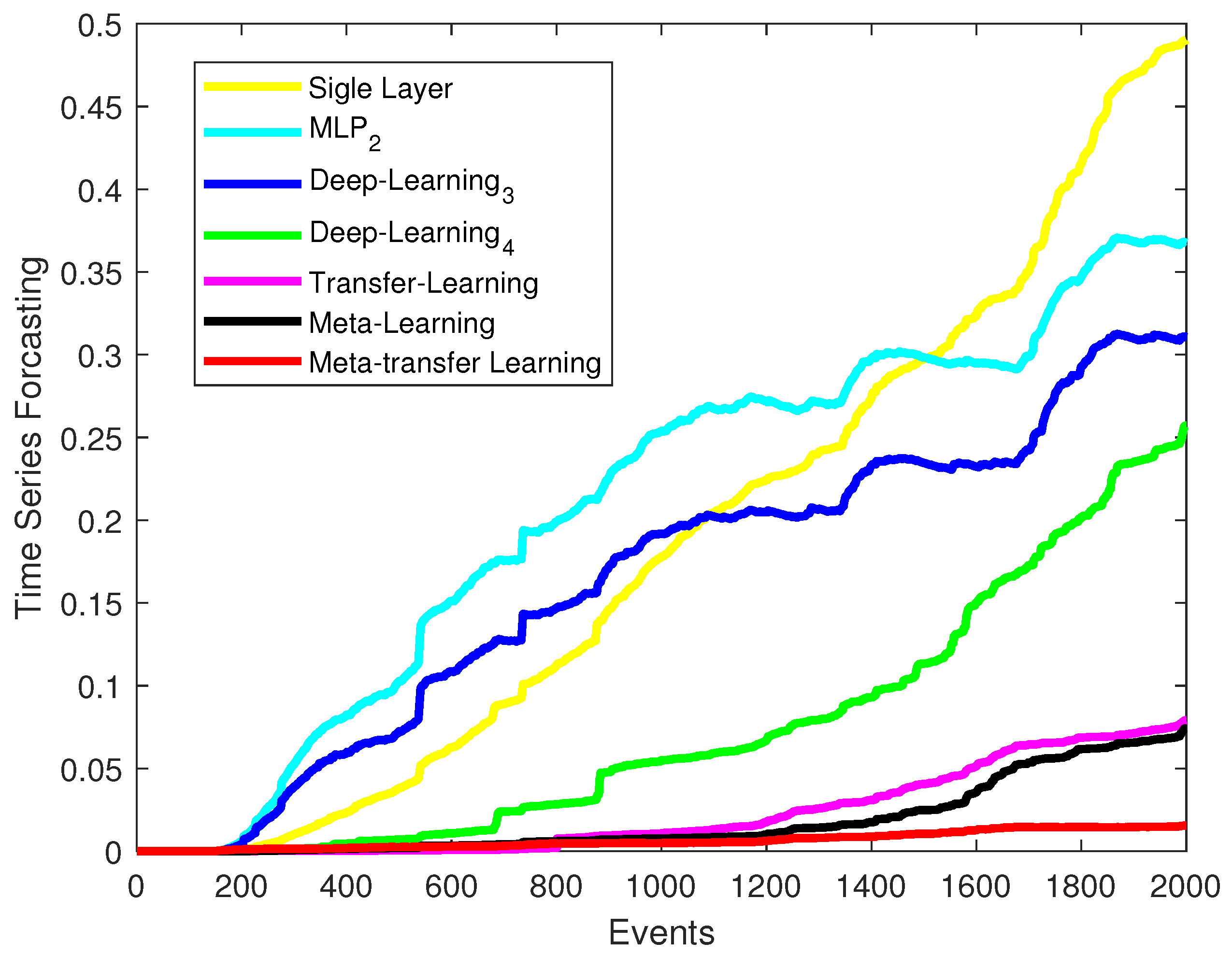
4.4. Comparison with Other Methods

The initial weights for all NNs are random in $\left[-1,1\right].$ The active function are sigmoid functions.

There are 1100 training data that are in April 2020. As discussed before, there are a lot of glitches or loss data in the training dataset. The failure rate is about $23\%$. The neural models are used to make a 150-day prediction. There are 2000 test data that are in September 2020. Figure 12 shows 200 data in the test phase.

The comparison results of PM10 forecasting are shown in Figure 13. So, the prediction errors increase with time, because it is difficult for the long-term prediction. But meta-transfer leaning has big advantages than the other neural models when the training datasets are not ideal.

The proposed method is compared with the following baseline models:

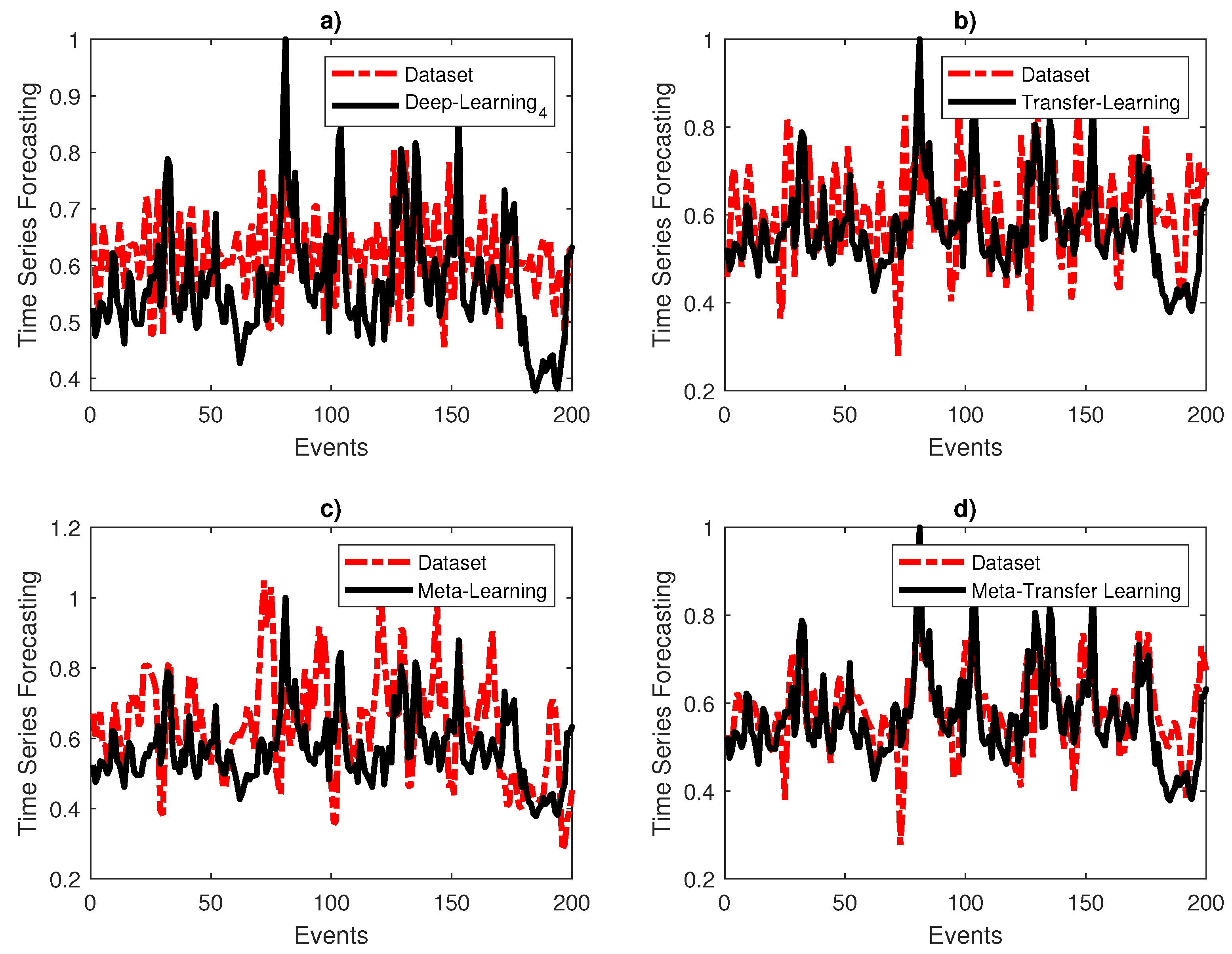
• Single-Layer Neural Network (NN) [3]: This network has one hidden layer with 10 neurons (${\mathrm{\Pi }}_{10\times 1}$).
• MutiLayer Perceptron (MLP) [3]: This network has two hidden layers, with 10 and 35 neurons, respectively (${\mathrm{\Pi }}_{10\times 35\times 15\times 1}$).
• Deep Neural Network (DNN1) [24], ${\mathrm{\Pi }}_{10\times 5\times 6\times 3\times 5\times 1}$: DNN1 has four hidden layers
• Deep Neural Network (DNN2) [24], ${\mathrm{\Pi }}_{10\times 70\times 60\times 35\times 1}$: DNN2 has three hidden layers
• Bayesian Inference with neural networks (Bayesian) [34]: This network uses the same deep neural network architecture as DNN1.
• Meta-transfer learning (MTL) [4]: This network uses the same deep neural network architecture as DNN1.
• Proposed mothed in this paper (BayesianGAN): GAN with Bayesian inference.

All data were normalized using the following equation:

$$x_k=\frac{x_k-min\left\{x_k\right\}}{max\left\{x_k\right\}-min\left\{x_k\right\}}$$

(34)

where $x_k$ is the data point, $min\left\{x_k\right\}$ is the minimum value in the dataset, and $max\left\{x_k\right\}$ is the maximum value in the dataset.

All neural networks were initialized with random weights uniformly distributed between $-1$ and 1. The activation function used for all hidden layers was the sigmoid function.

The training dataset consisted of 1100 data points from April 2020. As mentioned earlier, these data contained missing values, resulting in a failure rate of approximately $23\%$. Despite these challenges, we used neural network models to perform 150-day predictions. The test dataset comprised 2000 data points from September 2020. Figure 12 displays 200 data points from the test phase for visual comparison.

Figure 13 (with the corresponding figure caption) illustrates the comparison of PM10 forecasting performance for different models. As expected, prediction errors tend to increase with longer prediction horizons due to the inherent difficulty of long-term forecasting. However, our proposed meta-transfer learning approach (MTL-DNN3) demonstrates significant advantages over other neural network models, particularly when dealing with non-ideal training datasets with missing values.

The following metrics are used to compare forecasting errors:

$$\begin{array}{c}MSE=\frac{1}{N}\sum _i^N{e}_k^2\hfill \\ MAPE=\frac{1}{N}\sum _i^N\left|\frac{e_k}{x_k}\right|\hfill \end{array}$$

(35)

where $e_k$ is the prediction error at time step $k+150$ ($x_{k+150}-{\widehat{x}}_{k+150}$), and N is the total number of data points in the test set ($N=2000)$. The Mean Absolute Error (MAE) is the average absolute difference between predicted and actual values. The Mean Absolute Percentage Error (MAPE) indicates the sensitivity to outliers.

Table 2. Prediction errors.

Neural Model	MSE	MAPE
NN	$490.2$	$35.4$
MLP	$367.5$	$27.1$
DNN1	$310.8$	$30.1$
DNN2	$257.1$	$21.4$
Bayesian	$79.3$	$15.3$
MTL	$74.5$	$17.7$
BayesianGAN	$15.6$	$5.9$

summarizes the testing errors for all models. The table allows for a quantitative comparison of the performance across different models.

5. Conclusions

This paper presented a novel time series forecasting framework that leverages the power of Generative Adversarial Networks (GANs) and Bayesian inference to address the challenge of missing data. Our approach utilizes a C-GAN to realistically impute missing values in the time series, which is followed by Bayesian inference to quantify the uncertainty associated with the forecasts. This combined strategy offers several advantages:

(1) Improved Accuracy: By imputing missing values with realistic data, the framework provides a more complete picture for the forecasting model, leading to more accurate predictions.

(2) Uncertainty Quantification: Bayesian inference allows us to estimate the level of confidence in the forecasts, which is particularly important when dealing with missing data. Users can interpret the predictions alongside the associated uncertainty for better decision making.

(3) Robustness: The framework demonstrates robustness in handling real-world datasets with missing values, as shown in the application to air pollution forecasting in Mexico City.

Here are some limitations of the paper: (1) GAN can be susceptible to overfitting, especially with limited data. (2) Interpreting the GAN’s imputation process can be challenging. (3) The method cannot explicitly address how uncertainty arises due to missing data. (4) Training GANs can be computationally expensive in terms of time and resources.

This framework has the potential to be applied to various time series forecasting tasks where missing data are a concern. Further research directions include the following: (1) exploring different GAN architectures and hyper-parameter tuning to optimize the imputation process; (2) investigating the application of this framework to other time series forecasting problems beyond air pollution; and (3) developing methods for incorporating additional information sources, such as weather data, to potentially enhance forecasting accuracy.

References

1. Lu, P.; Ye, L.; Tang, Y.; Zhao, Y.; Zhong, W.; Qu, Y.; Zhai, B. Ultra-short-term combined prediction approach based on kernel function switch mechanism. Renew. Energy 2021, 164, 842–866. [Google Scholar] [CrossRef]
2. Mushtaq, M.; Akram, U.; Aamir, M.; Ali, H.; Zulqarnain, M. Neural Network Techniques for Time Series Prediction: A Review. Int. J. Inform. Vis. 2019, 3, 314–320. [Google Scholar] [CrossRef]
3. Hooyberghs, J.; Mensink, C.; Dumont, G.; Fierens, F.; Brasseur, O. A neural network forecast for daily average PM10 concentrations in Belgium. Atmos. Environ. 2005, 39, 3279–3289. [Google Scholar] [CrossRef]
4. Maya, M.; Yu, W.; Li, X. Time series forecasting with missing data using neural network and meta-transfer learning. In Proceedings of the 2021 IEEE Symposium Series on Computational Intelligence (SSCI 2021), Orlando, FL, USA, 5–7 December 2021; pp. 1–6. [Google Scholar]
5. Zhang, L.; Zhang, D. Domain Adaptation Extreme Learning Machines for Drift Compensation in E-Nose Systems. IEEE Trans. Instrum. Meas. 2015, 64, 1790–1801. [Google Scholar] [CrossRef]
6. Ye, R.; Dai, Q. A novel transfer learning framework for time series forecasting. Knowl.-Based Syst. 2018, 156, 74–99. [Google Scholar] [CrossRef]
7. Goodfellow, I.; Pouget-Abadie, J.; Mirza, M.; Xu, B.; Warde-Farley, D.; Ozair, S.; Courville, A.; Bengio, Y. Generative adversarial nets. In Proceedings of the Advances in Neural Information Processing Systems, Montreal, QC, Canada, 8–13 December 2014; Volume 27. [Google Scholar]
8. Isola, P.; Zhu, J.Y.; Zhou, T.; Efros, A.A. Image-to-image translation with conditional adversarial networks. In Proceedings of the IEEE Conference on Computer Vision and Pattern Recognition, Honolulu, HI, USA, 21–26 July 2017; pp. 1125–1134. [Google Scholar]
9. Yu, Y.; Srivastava, A.; Canales, S. Conditional lstm-gan for melody generation from lyrics. ACM Trans. Multimed. Comput. Commun. Appl. (TOMM) 2021, 17, 1–20. [Google Scholar] [CrossRef]
10. Fan, B.; Lu, X.; Li, H.X. Probabilistic inference-based least squares support vector machine for modeling under noisy environment. IEEE Trans. Syst. Man Cybern. Syst. 2016, 46, 1703–1710. [Google Scholar] [CrossRef]
11. Gernoth, K.A.; Clark, J.W. Neural networks that learn to predict probabilities: Global models of nuclear stability and decay. Neural Netw. 1995, 8, 291–311. [Google Scholar] [CrossRef]
12. Horger, F.; Würfl, T.; Christlein, V.; Maier, A. Deep learning for sampling from arbitrary probability distributions. arXiv 2018, arXiv:1801.04211. [Google Scholar]
13. Billings, S.A. Nonlinear System Identification: NARMAX Methods in the Time, Frequency, and Spatio-Temporal Domains; Wiley: Hoboken, NJ, USA, 2013. [Google Scholar]
14. Ratliff, L.J.; Burden, S.A.; Sastry, S.S. Characterization and computation of local Nash equilibria in continuous games. In Proceedings of the 2013 51st Annual Allerton Conference on Communication, Control, and Computing (Allerton), Monticello, IL, USA, 2–4 October 2013; pp. 917–924. [Google Scholar] [CrossRef]
15. Goodfellow, I. Nips 2016 tutorial: Generative adversarial networks. arXiv 2016, arXiv:1701.00160. [Google Scholar]
16. Dirección de Monitoreo Atmosférico, S.d.M.A. Technical Report, Secretaría del Medio Ambiente de la Ciudad de México. 2020. Available online: http://www.aire.cdmx.gob.mx/default.php (accessed on 20 March 2024).
17. Wu, W.; Zhang, N.; Li, Z.; Li, L.; Liu, Y. Convergence of the gradient method with momentum for back-propagation neural networks. J. Comput. Math. 2008, 26, 613–623. [Google Scholar]
18. Cortina-Januchs, M.G.; Quintanilla-Dominguez, J.; Vega-Corona, A.; Andina, D. Development of a model for forecasting of PM10 concentrations in Salamanca, Mexico. Atmos. Pollut. Res. 2015, 6, 626–634. [Google Scholar] [CrossRef]
19. Cabaneros, S.M.; Calautit, J.K.; Hughes, B.R. A review of artificial neural network models for ambient air pollution prediction. Environ. Model. Softw. 2019, 119, 285–304. [Google Scholar] [CrossRef]
20. Chaloulakou, A.; Grivas, G.; Spyrellis, N. Neural network and multiple regression models for PM10 prediction in Athens: A comparative assessment. J. Air Waste Manag. Assoc. 2003, 53, 1183–1190. [Google Scholar] [CrossRef]
21. Corani, G. Air quality prediction in Milan: Feed-forward neural networks, pruned neural networks and lazy learning. Ecol. Model. 2005, 185, 513–529. [Google Scholar] [CrossRef]
22. Grivas, G.; Chaloulakou, A. Artificial neural network models for prediction of PM10 hourly concentrations, in the Greater Area of Athens, Greece. Atmos. Environ. 2006, 40, 1216–1229. [Google Scholar] [CrossRef]
23. Chelani, A.B.; Gajghate, D.; Hasan, M. Prediction of ambient PM10 and toxic metals using artificial neural networks. J. Air Waste Manag. Assoc. 2002, 52, 805–810. [Google Scholar] [CrossRef]
24. Perez, P.; Reyes, J. An integrated neural network model for PM10 forecasting. Atmos. Environ. 2006, 40, 2845–2851. [Google Scholar] [CrossRef]
25. Papanastasiou, D.K.; Melas, D.; Kioutsioukis, I. Development and assessment of neural network and multiple regression models in order to predict PM10 levels in a medium-sized Mediterranean city. Water Air Soil Pollut. 2007, 182, 325–334. [Google Scholar] [CrossRef]
26. Cai, M.; Yin, Y.; Xie, M. Prediction of hourly air pollutant concentrations near urban arterials using artificial neural network approach. Transp. Res. Part D Transp. Environ. 2009, 14, 32–41. [Google Scholar] [CrossRef]
27. McKendry, I.G. Evaluation of Artificial Neural Networks for Fine Particulate Pollution (PM10 and PM2.5) Forecasting. J. Air Waste Manag. Assoc. 2002, 52, 1096–1101. [Google Scholar] [CrossRef] [PubMed]
28. Hrust, L.; Klaić, Z.B.; Križan, J.; Antonić, O.; Hercog, P. Neural network forecasting of air pollutants hourly concentrations using optimised temporal averages of meteorological variables and pollutant concentrations. Atmos. Environ. 2009, 43, 5588–5596. [Google Scholar] [CrossRef]
29. Paschalidou, A.K.; Karakitsios, S.; Kleanthous, S.; Kassomenos, P.A. Forecasting hourly PM10 concentration in Cyprus through artificial neural networks and multiple regression models: Implications to local environmental management. Environ. Sci. Pollut. Res. 2011, 18, 316–327. [Google Scholar] [CrossRef] [PubMed]
30. Fernando, H.J.S.; Mammarella, M.C.; Grandoni, G.; Fedele, P.; Marco, R.D.; Dimitrova, R.; Hyde, P. Forecasting PM10 in metropolitan areas: Efficacy of neural networks. Environ. Pollut. 2012, 163, 62–67. [Google Scholar] [CrossRef] [PubMed]
31. Perez, P. Combined model for PM10 forecasting in a large city. Atmos. Environ. 2012, 60, 271–276. [Google Scholar] [CrossRef]
32. Nejadkoorki, F.; Baroutian, S. Forecasting PM10 in metropolitan areas: Efficacy of neural networks. Int. J. Environ. Res. 2012, 6, 277–284. [Google Scholar]
33. Liu, W.; Li, X.; Chen, Z.; Zeng, G.; León, T.; Liang, J.; Huang, G.; Gao, Z.; Jiao, S.; He, X.; et al. Land use regression models coupled with meteorology to model spatial and temporal variability of NO2 and PM10 in Changsha, China. Atmos. Environ. 2015, 116, 272–280. [Google Scholar] [CrossRef]
34. Jorge Morales, W.Y. Improving Neural Network’s Performance Using Bayesian Inference. Neurocomputing 2015, 461, 319–326. [Google Scholar] [CrossRef]
Figure 1. Time series forecasting using neural networks. Here, x k + m is m-step ahead prediction. x ^ k + m is the neural network approximation of x k + m x k is the time series. x ¯ k is the missing data.
Information 15 00222 g001
Figure 2. Transfer learning for neural network training. Here, x k + m is m-step ahead prediction. x ^ k + m is the neural network approximation of x k + m Λ a and Λ b are different datasets. x k is the time series of x k . x ¯ k is the missing data of Λ a .
Information 15 00222 g002
Figure 3. Learning the underlying distribution with Conditional GAN. Here, x k + m is m-step ahead prediction. x ^ k + m is the neural network approximation of m-step ahead prediction, x k is the time series, and Z is random noise.
Information 15 00222 g003
Figure 4. The learning process of a Generative Adversarial Network (GAN) is visualized. The real distribution of x k + m is represented in black ( p T ). The green line depicts the generator’s distribution ( p G ) in. The blue line shows the discriminator’s distribution ( p D ). Training starts at point (a) and progresses toward point (d), (b,c) are intermediate points in the training process. Ideally, after training, the generator’s distribution ( p G ) approaches the real data distribution ( p T ) and the discriminator’s distribution ( p D ) approaches zero.
Information 15 00222 g004
Figure 5. Bayesian inference for forecasting. Here, p x k y k is the liklihood, p x k is the prior (from the GAN model), and p y k x k is the posterior.
Information 15 00222 g005
Figure 6. Environmental monitoring network in Mexico City. The digital number displayed here is the station number.
Information 15 00222 g006
Figure 7. Failures of the monitoring stations in 2020.
Information 15 00222 g007
Figure 8. Distribution of truth space gains.
Information 15 00222 g008
Figure 9. Distributions of gains.
Information 15 00222 g009
Figure 10. Forecasting results of the station ATI.
Information 15 00222 g010
Figure 11. Forecasting results of the station PED.
Information 15 00222 g011
Figure 12. P M 10 forecasting. (a) DNN, (b)TL-DNN3, (c) ML-DNN3, (d) MTL-DNN3.
Information 15 00222 g012
Figure 13. Testing errors of different neural models.
Information 15 00222 g013