


Abstract
This study estimates how alternative electric vehicle (EV) adoption pathways translate into fleet stock and electricity requirements in Türkiye through 2030. The available sales record contains only 12 annual observations for 2014–2025, including sharp recent acceleration. This information is insufficient to establish the value of a high-capacity recurrent network. We therefore compare parsimonious extrapolations on a fixed 2022 origin and treat the previously reported LSTM-derived pathway solely as an unvalidated scenario input. Newly calculated linear-trend, drift, and last-increment benchmarks supplement persistence and the retained ARIMA evaluation. The last-increment rule and ARIMA have almost identical holdout RMSEs of 140,335 and 140,336 vehicles, respectively; all methods substantially underpredict 2023–2025 sales. Under the lower-adoption reference pathway, zero retirements, and explicit vehicle-use assumptions, the 2030 stock reaches 1,406,522 vehicles. Annualized grid-side energy is 3375.65 GWh, equivalent to 0.847% of the national demand reference; uniform within-year entry reduces the calendar-year estimate to 3125.55 GWh. The alternative ARIMA extrapolation yields 3,528,590 vehicles and 8468.62 GWh. Sensitivities examine adoption, mileage, efficiency, fleet composition, retirement, and charging timing. The contribution is a transparent conditional stock-to-energy assessment, not evidence of LSTM superiority or a validated national adoption forecast.
1. Introduction
Low-carbon transport strategies increasingly rely on electric vehicles (EVs) to improve vehicle energy efficiency and reduce direct dependence on petroleum fuels. Wider EV adoption also creates a closer link between transport demand and electricity-system planning. Conventional vehicles obtain their operating energy from liquid fuels, whereas EVs draw some or all of that energy from electricity supplied through charging. Fleet growth therefore affects both annual electricity consumption and the timing of electricity demand. The environmental outcomes depend partly on the electricity supply mix, while the operational consequences depend on when and where charging occurs. Charging concentrated in existing high-demand periods can increase pressure on the electricity system even when its contribution to annual consumption remains modest [1,2,3].
Türkiye is a relevant setting for examining these relationships because its automotive market has changed rapidly. Rising EV sales have coincided with a wider availability of electric models, domestic production, developments in charging infrastructure, and changing market conditions. These developments make charging-related electricity demand an important consideration for system operators, policymakers, charging-network developers, and energy planners [4,5]. Continued adoption would expand the fleet that requires charging, but neither its future size nor its growth rate is certain. National annual energy requirements and local or time-specific loading should therefore be examined separately. A small annual energy share does not, by itself, establish that charging can be accommodated at every location and time [6,7].
EV sales forecasting and electricity accounting require different evidence. Statistical trends provide transparent baselines, while flexible recurrent methods require sufficient temporal information and credible out-of-sample gains. Published LSTM applications to adoption and charging [8,9,10,11] motivate methodological comparison but do not establish suitability for this study’s 12 annual observations. We therefore evaluate simple extrapolations directly and keep the inherited neural trajectory separate from verified forecast performance. Sales then enter an explicit stock-to-energy calculation [6,12].
The relationship between EV penetration and electricity demand depends on fleet size, annual distance traveled, vehicle efficiency, charging efficiency, and charging behavior. A framework that represents these factors explicitly can separate the effect of adoption from the assumptions used to translate adoption into energy demand. It can also examine departures from a reference trajectory. Scenario analysis helps evaluate the consequences of different adoption rates, but the resulting range should not be interpreted as a probability interval unless uncertainty has been estimated accordingly. International energy outlooks similarly distinguish historical observations from conditional future pathways [13,14].
Public automotive and electricity datasets provide a basis for assessing these relationships in Türkiye. The Automotive Distributors and Mobility Association (ODMD) publishes vehicle-market information. Our World in Data (OWID) provides internationally comparable EV sales and stock indicators, including series derived from the International Energy Agency (IEA) [15,16,17]. Energy Exchange Istanbul (EPİAŞ) provides electricity-market and demand information through its Transparency Platform and associated web services [18,19]. These sources cover different concepts and reporting intervals. Their integration therefore requires consistent definitions of sales, registered stock, vehicle categories, and electricity consumption, rather than treating every series as interchangeable.
This study connects these stages within a Türkiye-specific assessment. Its central question is how a reference trajectory of EV sales translates into accumulated vehicle stock and, under stated operating assumptions, into annual electricity requirements through 2030. A related question concerns the sensitivity of those requirements to alternative adoption levels and charging-time allocations. The distinction matters during a period of rapid market change because annual sales forecasts, stock penetration projections, and charging-energy calculations address different planning questions. The framework keeps these quantities separate throughout the analysis.
The forecast assessment uses a common 2022 origin to compare persistence, drift, ordinary least-squares (OLS) linear trend, last-increment extrapolation, and the retained ARIMA predictions. The original inconsistent model-error table is excluded from the revised evidence. No independently verifiable LSTM holdout predictions are available, so its five future values serve only as a conditional lower-adoption pathway. A full-series ARIMA extrapolation provides a contrasting pathway; neither is designated the most likely forecast. The same stock and energy equations are applied to both.
This study contributes a transparent connection between adoption assumptions, accumulated stock, and electricity requirements. Section 2 provides focused background; Section 3 defines the data, parsimonious benchmarks, and accounting; Section 4 reports the diagnostic and scenario results; Section 5, Section 6 and Section 7 discuss their interpretation, limitations, and conclusions. The analysis makes no claim of algorithmic novelty or demonstrated deep-learning advantage.
2. Literature Review
2.1. EV Adoption and Electricity Demand
EV adoption links changes in the vehicle fleet to changes in electricity demand. Battery electric vehicles (BEVs) obtain their driving energy from batteries, whereas plug-in hybrid electric vehicles (PHEVs) combine electrically powered travel with fuel-based operation. As these vehicles replace internal combustion engine (ICE) vehicles, part of transport energy demand shifts from liquid fuels to electricity. The magnitude and temporal profile of that shift depend on fleet composition, driving activity, battery and vehicle characteristics, and charging practices. Its environmental consequences also depend on electricity generation and the wider energy system [1,2]. These distinctions matter when a combined BEV–PHEV adoption series is translated into electricity requirements.
Previous studies examine EV charging at national, regional, and distribution-network scales. Reviews describe a range of potential effects, including additional energy consumption, coincident peak demand, voltage constraints, and changes in network loading [20,21,22]. Studies of local charging show that concentrated or uncoordinated demand can affect residential loads and distribution networks, while coordinated charging can alter the timing of demand [23,24]. The importance of each effect depends on adoption, infrastructure, and the distribution of charging activity. A small national annual energy share should therefore not be interpreted as evidence that additional generation, transmission, distribution, or charging capacity will never be required.
Annual sales alone cannot represent these cumulative electricity requirements. A vehicle sold in one year continues to consume electricity in subsequent years, so the relevant quantity for energy demand is the stock in operation rather than the current year’s sales. Stock formation depends on new registrations and on vehicles leaving the fleet. Adoption forecasts, stock estimates, and electricity-use calculations therefore require separate definitions and an explicit accounting relationship. This distinction is particularly important in a rapidly expanding market, where a high growth rate in new sales may coexist with a much smaller share of the total active fleet [6,12].
2.2. EV Sales and Penetration Forecasting
EV adoption has been modeled using diffusion, econometric, time-series, and machine-learning approaches [4,8,13]. Their relevance depends on the available observations and forecast horizon. A smooth projected curve does not itself justify a complex model: a constant sales flow creates linear stock accumulation by construction. The empirical question here is whether a more elaborate extrapolation improves on simple trend rules for the observed annual sales target.
Non-seasonal ARIMA and simple trend methods are natural benchmarks for annual data. Annual aggregation prevents within-year seasonality from being identified in this record. All evaluated forecasts therefore use the same sales target, information cutoff, and three holdout years. A post hoc piecewise-linear fit using future observations would not provide a valid forecasting comparison; breakpoint estimation would also consume scarce degrees of freedom.
Tree-based models require explicitly constructed lagged inputs. Cross-domain comparisons of regression, tree-based, and hybrid methods [25,26] illustrate methodological alternatives, but do not justify model complexity in this annual national series. RF and XGBoost are not included in the revised performance ranking because their observation-level holdout predictions are unavailable.
2.3. Recurrent Models and Data Requirements
LSTM gates provide a flexible representation of sequential dependence [9]. Applications to charging behavior, short-term charging demand, and traffic [10,11,27] concern different targets and information volumes. With a two-year input window, the seven-year training partition in this study supplies only five overlapping training sequences. That effective sample is inadequate to demonstrate the value of the documented 32-unit network [28,29,30].
Convolutional Neural Networks (CNNs) and Transformer architectures offer alternative approaches to time-series forecasting, particularly when the analysis involves complex temporal patterns, extensive sequential observations, or multiple interacting variables [31]. However, their inclusion was not essential to the objectives of the present study, which focused on evaluating EV adoption trajectories and translating them into electricity-demand scenarios through a transparent forecasting and accounting framework. The selected methods provided complementary perspectives on historical trends, temporal dependencies, and future adoption pathways. Given the annual structure of the available dataset, introducing additional deep-learning architectures would have required a separate experimental design and validation strategy beyond the scope of this analysis. Therefore, CNNs and Transformers were not included, while their potential application to higher-resolution EV adoption and charging datasets remains a relevant direction for future research.
2.4. Electricity-Demand Forecasting Related to EV Charging
Conventional electricity-demand forecasting relates consumption to historical demand, weather, calendar effects, economic activity, and other drivers. EV charging introduces a transport-related component whose timing and magnitude depend on vehicle use and charging access. This component need not follow the temporal patterns of other electricity uses. Studies that incorporate weather, traffic, and user characteristics illustrate the importance of these contextual influences on charging demand [32,33,34]. Long-term fleet-based energy estimates and short-term charging-load forecasts consequently serve different purposes and require different levels of temporal detail.
EV electricity-demand studies fall into two broad groups. Bottom-up approaches derive consumption from the number of vehicles, annual distance, energy use per kilometer, battery-related characteristics, and charging losses. Charging-event approaches use observations of charging activity to estimate or forecast demand at a finer temporal or spatial scale [11,35]. Bottom-up accounting suits long-term scenarios in which future fleet sizes are of interest but detailed charging records are unavailable. Its transparency also makes the dependence on operating assumptions visible. It does not replace hourly load modeling or provide a direct test of charging-control performance.
Converting penetration into electricity demand requires more than a projected percentage of the vehicle fleet. At a given stock level, demand changes with driving distance and energy consumption per kilometer. For PHEVs, the electrically driven share of distance is an additional determinant. Charging efficiency distinguishes the electricity supplied by the grid from the energy delivered to the vehicle. These quantities must be kept separate when comparing annual energy or peak-period power [6,24]. A fleet-average calculation can support a simplified scenario, but it cannot describe variation across vehicle models, seasons, locations, or driving conditions.
Charging behavior determines when the annual energy requirement appears on the electricity system. Charging immediately after vehicles return home may coincide with the evening peak, whereas delayed or coordinated charging can shift consumption to other periods. The literature distinguishes local and centralized strategies, home energy management, and methods that account for user preferences and distribution-network conditions [23,36,37,38]. Reviews of vehicle-to-grid and charging strategies describe wider integration options [39,40]. These studies motivate charging-time scenarios, but an assumed allocation of energy across hours is not equivalent to implementing and validating one of these control methods.
2.5. Scenario Analysis of EV Penetration
Long-term EV adoption depends on technology, purchase prices, charging infrastructure, preferences, energy costs, taxation, incentives, and regulation. A single deterministic trajectory cannot capture every combination of these influences. Scenario analysis instead evaluates the consequences of specified alternative assumptions. International outlooks use conditional pathways to examine vehicle-market development and energy demand [6,13,14]. For EV electricity requirements, scenarios can vary fleet size, driving activity, electricity consumption per kilometer, charging efficiency, or the temporal distribution of charging. Their interpretation depends on whether the assumed changes are empirically calibrated or chosen to explore sensitivity.
Conservative, baseline, and accelerated adoption scenarios offer a transparent way to distinguish slower, reference, and faster fleet development. Applying the same energy-accounting model to each scenario isolates the consequences of the assumed adoption level. These labels describe the ordering of the cases, not their probabilities. A conservative case is not necessarily a lower confidence bound, and an accelerated case is not necessarily the most likely outcome under a particular policy. The magnitude of the scenario adjustments should therefore remain explicit when the results inform discussions of infrastructure or electricity-system planning.
Linking scenarios to an identified reference trajectory makes the accounting transparent, but it does not establish the forecast validity of that trajectory. The present analysis distinguishes a 25% change in future sales from a 25% change in total 2030 stock. The former preserves the common starting fleet, whereas the latter is a direct terminal-stock sensitivity. Neither is a statistically estimated prediction interval or an independently validated policy pathway.
2.6. EV Transition in Türkiye
Türkiye’s automotive transition provides a specific context for studying the relationship between EV adoption and electricity demand. Domestic electric-car production, a wider range of imported models, and improved charging availability have accompanied changes in the market [4,5]. These conditions can influence future adoption, but this analysis does not estimate their individual causal effects. The relationship between EV sales and total passenger-car sales may continue to change. It is therefore important to distinguish the current market share from cumulative stock penetration and to avoid extrapolating recent growth without qualification.
ODMD publishes monthly and annual automotive-market reports that support the construction of sales and market-share indicators [5]. OWID provides internationally comparable EV series based on IEA data, including separate sales and stock products [15,16]. The IEA data product provides further documentation for international comparisons [17]. Differences in vehicle coverage, revision schedules, and reporting concepts must be considered when these sources are combined. Agreement in an overall trend does not establish equivalence between BEV-only registrations, combined BEV–PHEV sales, and cumulative vehicle stock.
EPİAŞ provides electricity-market information through its Transparency Platform and web services [18,19]. These resources support the characterization of electricity consumption and of the denominator used to express EV-related energy as a national share. The resolution of the extracted electricity data should match the analytical question. Annual totals suit annual energy accounting, whereas assessing coincident system peaks requires observations or assumptions at a much finer time scale. Combining electricity and automotive data is therefore useful only when these distinct measurement requirements remain explicit.
The Türkiye-specific motivation is to connect market development with future electricity requirements in a single, traceable calculation. Market growth, charging infrastructure, environmental implications, and grid integration are related but separate topics. The present framework focuses on the chain from sales to stock and from stock to annual charging energy, supplemented by adoption and charging-time scenarios. It does not assume that existing Turkish research has ignored this relationship, and the integration alone does not constitute methodological novelty. Its value depends on the transparency of the accounting and the credibility of the underlying data and assumptions.
2.7. Research Gap and Motivation
The literature includes substantial work on EV adoption, electricity-demand forecasting, charging-load modeling, and grid integration. These research areas overlap, but they do not always use the same target variables or time horizons. An adoption model can forecast new sales without estimating the resulting fleet energy requirement. An aggregate electricity forecast can represent historical consumption without isolating future EV charging. A bottom-up charging study can rely on externally defined adoption scenarios rather than estimating a reference trajectory. Bringing these stages together requires clear links among the forecast target, stock accounting, energy parameters, and scenario definitions.
The methodological motivation is integration with explicit boundaries, not new component algorithms. Integrated decision-support approaches also occur in other resource domains [41], but their success does not validate this forecast. The present framework distinguishes annual sales from operating stock, sales share from stock penetration, and annual energy from charging-window average power.
The numerical contribution is conditional energy accounting supported by an explicit examination of forecast limitations. The inherited LSTM-derived pathway is one input case, not a selected model. Parsimonious holdout benchmarks assess what can be learned from the short sales record; the ARIMA extrapolation provides a contrasting accounting case without establishing predictive superiority.
The framework thus provides an accounting structure for relating transport-market projections to electricity-system questions. It can organize evidence on charging-energy requirements, infrastructure planning, and coordinated transport and electricity policy in Türkiye. Its outputs should be interpreted at the level the analysis supports: national annual energy scenarios and simplified charging-time illustrations. Regional network adequacy, actual peak demand, policy effectiveness, and operational charging optimization require additional evidence and models beyond this scope.
3. Materials and Methods
3.1. Analytical Scope and Evidence Boundary
The central objective is to quantify how an EV sales trajectory, the accumulated passenger-car stock, and vehicle-use assumptions translate into electricity requirements in Türkiye through 2030. The analysis keeps three kinds of evidence separate: historical and benchmark quantities taken from the archived study record, accounting outputs calculated from explicitly stated inputs, and externally documented parameters or official projections used for sensitivity comparisons.
The forecasting target is annual EV sales during 2014–2025. We examine whether the data support anything beyond simple trend extrapolation before interpreting the 2026–2030 pathways. The five inherited LSTM-derived values are retained only to preserve a transparent lower-adoption accounting case; all stock and energy results could be recalculated from any explicitly supplied sales path. The alternative ARIMA path uses identical downstream assumptions.
3.2. Data Sources, Measurement Definitions, and Chronology
ODMD market reports provide domestic passenger-car sales information [5]. OWID and IEA resources provide internationally comparable EV sales and stock indicators [15,16,17]. The sales definition includes BEVs and PHEVs. The historical stock series switches from a cumulative-sales reconstruction for 2014–2020 to registered electric passenger cars for 2021–2025. This switch is a break in measurement construction, not evidence of a market change. A registered electric-car count cannot automatically be equated with a combined BEV–PHEV stock, and non-plug-in hybrids are excluded from the electricity-accounting definition.
Electricity-market information is associated with the EPİAŞ Transparency Platform [18,19]. The annual national-demand reference for 2025 is 360,929 GWh. This value is an aggregate consumption denominator, not a charging-event dataset. The analysis uses no hourly charging records, weather-adjusted driving observations, or national measurements of PHEV electric driving.
For the stock-penetration denominator, the 2025 passenger-car population is 17,373,581 vehicles, as reported in the Eurostat passenger-car series by type of motor energy for Türkiye [42]. The category comprises passenger cars of all fuel types, not all road motor vehicles, annual new-car sales, or the light-commercial fleet. This count is extended under a 7% annual growth scenario. The 7% rate is a transparent scenario specification, not a parameter estimated in the forecasting experiment. Alternative rates of 4% and 10% test the dependence of penetration on this denominator.
The Ministry of Energy and Natural Resources reports 2025 gross electricity consumption of approximately 360.9 TWh and a National Energy Plan projection of 455.3 TWh for 2030 [43]. The rounded 2025 value is consistent with the 360,929 GWh reference. The official 2030 quantity serves as an alternative denominator, whereas the main 2% annual-growth case is an explicit assumption and is not presented as the Ministry’s forecast.
The record contains 12 annual observations. Table 1 distinguishes the original neural-development partition from the benchmark information set. The new deterministic baselines use all nine values from 2014–2022 and forecast 2023–2025 from a fixed end-2022 origin, without updating on holdout observations. The ARIMA predictions retained from the supplied manuscript use that same fitting period. Its order, however, was discussed using full-series AICc results; this revision does not claim a fully nested, test-independent ARIMA selection experiment. The full series is used only for the separate 2026–2030 extrapolation. No new LSTM training or validation is claimed.
Table 1.
Chronological data partitions and forecast-generation periods.
Data adequacy is assessed from the sampling frequency, the number of usable windows, and the observed annual increments. A two-year look-back within the seven-year neural training partition leaves five overlapping input–target sequences, not five independent long histories. For a standard single-bias LSTM with one input feature and 32 units, the recurrent layer contains 4 × 32 × (1 + 32 + 1) = 4352 trainable parameters; the dense output adds 33, giving 4385. This is an architecture-based count, not an inspection of a saved network. It shows the mismatch in scale between the documented capacity and available observations; it is not a formal generalization bound.
The statistical benchmark is specified as a non-seasonal ARIMA(1,1,0) model, consistent with the annual frequency of the series. For the 2026–2030 comparison trajectory, model selection was conducted using AICc over candidate orders (p, d, q), with p ≤ 2, d ∈ {0, 1}, and q ≤ 2, estimated by maximum likelihood on the 2014–2025 annual sales series. ARIMA(2,1,1) was excluded because it produced a degenerate solution, characterized by a boundary autoregressive coefficient of 1.0 and a zero forecast path. Among the remaining candidates, ARIMA(1,1,0) achieved the lowest AICc (266.22), followed by ARIMA(1,1,2) (267.68) and ARIMA(2,1,0) (267.95). The fitted ARIMA(1,1,0) model yielded an autoregressive coefficient of φ1 = 0.999404 (SE = 0.3031) and an innovation variance of σ2 = 1.151 × 10⁹ vehicles2. For the separate fixed-origin evaluation, ARIMA(1,1,0) was fitted exclusively to the 2014–2022 observations and used to forecast 2023–2025 (Section 4.2). These two fitting periods serve distinct purposes: the full historical series provides the 2026–2030 comparison trajectory, whereas the earlier training period supports an out-of-sample assessment without incorporating the test observations. Accordingly, the reported coefficients and forecasting errors are interpreted within their respective estimation periods.
Figure 1 shows the documented chronological partitioning, in which the 2023–2025 observations are reserved for out-of-sample evaluation.
Figure 1.
Documented chronological partitioning protocol for the annual EV sales dataset.
3.3. Forecasting Representation and Preprocessing
The forecasting framework uses chronological ordering rather than a random train–test allocation. In a reproducible implementation, each forecast may use only information available at its origin, including the scaler, lagged inputs, and any treatment of gaps. The archived record does not document the preprocessing that was executed, so the study claims neither interpolation nor a no-missing-data condition for the original model fits. The five annual scenario sales inputs used here, by contrast, are fully enumerated and complete, and their downstream processing requires no imputation or normalization.
The min–max transformation for continuous forecasting inputs is given in (1):
where yt is the sales value at time t, is its scaled value, and and are the minimum and maximum over the training set . A constant training series would require a separately specified transformation because the denominator is zero. Equation (1) defines the transformation; the scaler extrema of the original implementation were not archived.
For the ordered sequence {y1,…,yT} of EV sales, the sliding-window input and forecast target are
where T is the number of observations, L is the look-back length, h is the forecast horizon in observation intervals, ⊤ denotes transposition, and fθ is a model with parameters θ. With annual data, L = 2 corresponds to the two-year look-back used by the recurrent and tree-based models. A monthly window cannot be interpreted as an annual window.
3.4. Parsimonious Benchmarks and the Role of the Inherited LSTM
Model complexity is not warranted merely because the future path is smooth or the market may be nonlinear. We use four transparent deterministic rules: persistence, historical-average drift, OLS linear trend, and last-increment extrapolation. Persistence and drift are standard forecasting benchmarks [44]. The last-increment rule extends the final observed local slope and directly tests whether a simple linear continuation explains the ARIMA result. It is a sensitivity benchmark, not an estimated change-point model.
At the end-2022 origin, let T = 9, y1 = 68, yt = 7540 at t = T, and yt−1 = 3920. For h = 1, 2, 3, drift predicts yt + h(yt − y1)/(T − 1) = 7540 + 934 h; last-increment extrapolation predicts yt + h(yt − yt−1) = 7540 + 3620 h. OLS fits sales against t = 0, …, 8 by minimizing squared errors, yielding intercept −1361.4667 and slope 724.95 vehicles/year; predictions use t = 9, 10, 11. These formulas fully specify the new baselines and use no holdout outcomes for coefficient fitting.
The inherited LSTM specification is a single 32-unit recurrent layer, dropout 0.1, a dense scalar output, two-year look-back, Adam with learning rate 0.01, batch size 4, up to 500 epochs, early-stopping patience 50, and seed 42. These settings are documented for provenance only. Five training sequences and two validation years cannot support a persuasive tuning study. Dropout and early stopping may regularize fitting but do not demonstrate control of overfitting here. No saved weights, scaler extrema, learning curves, or observation-level holdout predictions are supplied, so neither reliable LSTM generalization nor superiority can be established.
The revised performance comparison contains only forecasts whose test values are disclosed. The retained ARIMA predictions are evaluated alongside the four deterministic rules; no LSTM, GRU, RF, or XGBoost performance ranking is inferred. The five inherited LSTM-derived future values remain an explicitly unvalidated scenario, not a forecast selected by accuracy. For annual data, seasonal persistence with period one reduces to ordinary persistence:
No ensemble models, automatic breakpoint searches, CNNs, Transformers, or additional recurrent architectures were included in the analysis. The dataset contained only 12 annual observations, which limited the feasibility of training and validating more complex models. Introducing these architectures would have increased model complexity and uncertainty in model selection without sufficient independent observations to support reliable evaluation. Table 2 distinguishes the evaluated baseline models from the previously developed neural scenario.
Table 2.
Evaluated benchmark rules and provenance of the inherited neural scenario.
The main objective was to examine whether the statistical extrapolation provided any predictive advantage over a straightforward continuation of the historical trend. However, the results should be interpreted within the limitations of the available data. They do not demonstrate that the evaluated models can reliably anticipate market transitions, nor does the three-year holdout provide sufficient evidence to establish forecasting reliability over a five-year horizon.
3.5. Error Metrics
For observed sales yi and predictions at n common forecast targets, the absolute and squared-error measures are defined in (4) and (5), and the percentage measures in (6) and (7):
MAE and RMSE are measured in vehicles. MAPE requires nonzero targets; all three holdout sales values are positive. For sMAPE, a zero–zero pair contributes zero. Errors are descriptive values on three common forecast targets; no confidence interval, significance test, or population-level model ranking is inferred. New baseline errors are calculated directly from the disclosed sales sequence; ARIMA errors are recalculated from its retained rounded predictions.
3.6. Stock Formation, Retirement, and Penetration
The stock identity distinguishes annual sales, or entries, from the number of vehicles in service. For year t, the accounting equations are
where St is the end-of-year EV stock, Nt is the annual entry to the modeled fleet, Rt is the number of vehicles retired or removed during the year, and r is the annual removal fraction applied to the preceding year-end stock. Sales are treated as entries, with no separately estimated registration lag, imports, or exports. The reference case uses r = 0, meaning no removals over 2026–2030. This setting is a short-horizon accounting convention, not an assertion of infinite vehicle lifetime. The sensitivity cases use r = 0.01, 0.03, and 0.05 as uncalibrated removal-rate scenarios.
With a common starting stock and a constant removal fraction, the equivalent cohort expression is
where u indexes the entry year and (1 − r)t−u is the surviving proportion of that cohort at the end of year t. New entrants are not subject to same-year retirement in this convention. No fixed lifetime, age-specific survival distribution, or estimated scrappage hazard is implied. Equation (10) serves as an independent arithmetic check of the recursion in (9).
The 2026 EV stock of 572,721 vehicles and annual sales of 207,877 imply an initial stock of 364,844 vehicles in 2025. This value serves as a conditional starting point for fleet-stock accounting rather than a verified national BEV–PHEV count. It is 5747 vehicles below the historical maximum of 370,591 reported in Section 4.1. The available records do not establish whether this difference results from vehicle-category coverage, reporting dates, or data inconsistencies. To assess its influence, an additional sensitivity case uses 370,591 vehicles as the initial stock. Applying Equation (8) to the projected annual sales yields an EV stock of 1,406,522 vehicles by 2030 under the reference assumptions.
EV stock penetration and the passenger-car denominator are
where Pt is EV stock penetration in percent, Vt is the total passenger-car stock, and gV is the assumed annual growth rate of the passenger-car population. All calculations use full-precision values, and rounding is applied only for reporting. The penetration estimates assume that the modeled EV stock and the total passenger-car population refer to consistent vehicle categories. They are therefore scenario-based penetration measures rather than verified national penetration rates.
The share of EVs in new sales is a different quantity:
where Mt is the new-sales share and At is the total passenger-car sales in the same year and category. Because the analysis does not project At, it does not forecast the new-sales share, and stock penetration is never used as a substitute for this market-share indicator.
3.7. Vehicle-Side and Grid-Side Electricity Accounting
The principal energy results report the full-year energy associated with the end-of-year stock. They are annualized fleet requirements and do not imply that every vehicle sold in that year operated for twelve months. A separate timing case approximates the average operating stock under uniform net entry through the year:
where is the mean of the beginning- and end-of-year stock. For the zero-retirement case, this mean is the exposure implied by uniform entry. It is not an estimate derived from registration dates. The reference calculation uses St, and the calendar-year sensitivity substitutes . The same choice applies consistently to vehicle-side energy, grid-side energy, and the average charging-window load.
To distinguish BEV and PHEV operation, the annual vehicle-side and grid-side electricity in GWh are defined as
where SB,t and SP,t are the BEV and PHEV stocks, dB and dP are the annual distances per vehicle in km/year, cB and cP are the vehicle-side electricity consumption per electrically driven kilometer in kWh/km, and fP is the fraction of PHEV distance driven electrically. The efficiencies ηB and ηP are the ratios of vehicle-side charging energy to grid-side energy. The factor 10−6 converts kWh to GWh. Charging losses enter once, through division by the efficiency, and upstream generation and network losses are outside the analytical boundary.
When mileage, consumption, and efficiency are common to both vehicle types, let q = SP,t/St be the PHEV share of the stock and f = fP. The fleet-composition factor and the simplified accounting are then
where F is the electrically driven fleet-equivalent fraction, d is the common annual distance, c is the common vehicle-side consumption per electric kilometer, and η is the common charging efficiency. The reference case uses F = 1, an all-electric-equivalent energy case. This choice does not assert that the combined sales series contains only BEVs or that PHEVs drive entirely on electricity. Because the observed fleet split is unavailable, the composition sensitivities set the PHEV stock share to an illustrative q = 0.20 and vary f across 0.10, 0.50, and 0.80, which gives F = 0.82, 0.90, and 0.96, respectively.
The electric-driving sensitivity reflects the substantial variation documented in European PHEV use. A 2022 study by the International Council on Clean Transportation (ICCT) and the Fraunhofer Institute reports electric-driving shares of approximately 45–49% for private vehicles and 11–15% for company vehicles [45]. These observations motivate testing low and intermediate fractions, and the 80% case represents a high electric-use scenario. Neither the European averages nor the assumed 20% PHEV stock share are presented as a measurement for Türkiye.
3.8. Operating Parameters, National Demand, and Energy Shares
The reference values of 12,000 km/year and 0.18 kWh/km are modeling assumptions, not estimated fleet averages for Türkiye. They imply 2160 kWh of annual vehicle-side energy per all-electric-equivalent vehicle. The 90% charging-efficiency assumption raises the corresponding grid requirement to 2400 kWh per vehicle. Vehicle models, driving conditions, temperature, charging power, and user behavior can change these quantities. The analysis examines their influence through mileage of 9000–18,000 km/year, consumption of 0.14–0.22 kWh/km, and efficiency of 80–95%. These are sensitivity ranges, not confidence bounds.
Charging efficiency is not universal. Experimental work by Reick et al. documents charging losses that depend on the tested vehicles and charging conditions [46]. This evidence supports explicit loss accounting and sensitivity analysis, but it does not establish 90% as a calibrated national mean. The model does not infer a distribution of battery sizes or efficiencies from a single average consumption parameter.
The national electricity-demand reference and the EV-to-national-demand ratio are
where Dt is the annual national electricity demand in GWh, gD is the assumed national-demand growth rate, and Qt is the ratio of EV grid energy to national demand in percent. The main case uses gD = 0.02, alternative cases use 0 and 0.04, and a separate case uses the official 2030 projection of 455,300 GWh directly [43]. The official value corresponds to about 4.76% annual growth from the 2025 baseline, but it is not attributed to a constant-growth model.
The national reference may already include electricity consumed by the existing EV fleet. Accordingly, Qt is a scale comparison, not the percentage increase caused by adding the entire projected fleet to a counterfactual demand series without EVs. The analysis never adds the full Egrid,t to a baseline that already contains EV charging. A net-increment estimate would require an explicitly defined counterfactual for existing EV demand and other loads.
3.9. Charging-Window and System-Peak Scenarios
The peak analysis allocates annual grid-side energy to a designated window on a representative average day. The successive conversions are
In (20), eday,t is the average daily grid-side energy in MWh/day. In (21), α is the share of daily charging energy assigned to the designated window, H is the daily window duration in hours, and Lt is the average grid-side power within that window in MW. In (22), K is the assumed national system peak in MW and It is the comparison ratio in percent. The 365-day convention applies to all cases for comparability; it is a representative-year normalization, not a leap-year charging calendar.
The three charging allocations are α = 0.60, 0.20, and 0.10, with H = 4 h/day. They represent peak-concentrated, lower-coincidence, and strongly shifted charging, respectively. The fractions and the four-hour window are not estimated national charging profiles. Two-hour and six-hour windows, together with the alternative fractions, quantify their effect. The illustrative K = 60,000 MW is neither a forecast by the Turkish Electricity Transmission Corporation (TEİAŞ) nor an observed 2030 peak, and comparison denominators of 50,000 and 75,000 MW are also tested.
At fixed energy and window duration, the reduction from the 60% allocation to the 10% allocation is
The subscripts in (23) identify the allocation fractions, not different observed controllers, and the result is scenario arithmetic. The analysis implements no charging optimizer, user-availability constraint, charger power limit, rebound-load test, or feeder model. The calculated average within the designated window is not an instantaneous system peak, and shifting energy out of that window does not prove that a new maximum is avoided elsewhere.
3.10. Scenario Design and Numerical Sensitivity Protocol
All sensitivity cases are deterministic recalculations of (8)–(23), using the five annual sales inputs and full-precision intermediate values. No historical data are resampled or imputed. Except for the two combined cases, each case changes only the named assumption or, for a PHEV case, the named composition specification. The accounting exercise evaluates the response to assumptions, not forecast-model robustness or the probability of a future outcome.
Two distinct adoption perturbations are used. A flow perturbation changes only future entries and retains the 2025 initial stock:
The multiplier μ applies uniformly to each annual EV sales input for 2026–2030, while the initial fleet stock remains unchanged. The terminal-stock sensitivity, in contrast, adjusts the projected 2030 EV stock directly without modifying the annual sales trajectory:
Here, κ scales the total 2030 stock and does not describe a complete, stock-conserving sales pathway. Separating the two perturbations prevents a reduction in future sales from implicitly removing a quarter of the starting fleet. Both sets of results are reported, so that the terminal-stock interpretation remains available alongside the more coherent flow perturbation. The 25% deviations are uncalibrated sensitivities, not conservative or accelerated confidence limits.
Additional regime scenarios hold annual sales at the reported 2025 level of 237,000 or increase that level by 10% or 20% per year over 2026–2030. The value of 237,000 is the source-reported annual figure. These trajectories are transparent alternatives to the near-flat LSTM-derived path; they are not ARIMA forecasts, refitted neural forecasts, or formal structural-break estimates.
For a common time convention, the energy response can be checked through the ratio
where primes identify an alternative case. This relationship provides an independent check of units and proportionality. It implies unit proportional responses to stock, distance, and consumption and an inverse response to efficiency; it does not imply empirically measured elasticities. Changing the electricity-demand denominator affects the national ratio but not EV energy or power. Changing the system-peak denominator affects only the peak comparison percentage. Changing the growth of the total passenger-car stock affects penetration, not charging energy. Table 3 lists the reference inputs and tested parameter ranges.
Table 3.
Reference inputs and tested parameter ranges for the accounting analysis.
The combined lower-energy case uses future sales multiplied by 0.75, 3% annual removals, 9000 km/year, 0.14 kWh/km, 95% charging efficiency, a 20% PHEV share with 10% electric distance, and 4% national-demand growth. The combined higher-energy case uses future sales multiplied by 1.25, zero removals, 18,000 km/year, 0.22 kWh/km, 80% charging efficiency, the all-electric-equivalent fleet, and zero national-demand growth. Both cases retain the reference four-hour window, the 60% allocation, and the 60,000 MW comparison peak. They are joint stress cases, not estimated bounds on likely demand. Every output is calculated from unrounded inputs. Integer reference stocks remain exact, and fractional vehicles in the removal and multiplier cases represent expected or scaled accounting stocks that are kept at full precision until display. Energy is reported in GWh or TWh, with 1 TWh = 1000 GWh. The input values in Table 3 and the numbered equations are sufficient to reproduce every accounting result.
4. Results
4.1. Historical Reporting Coverage
The historical summaries span 2014–2025 and describe a period of rapid change in the scale of EV adoption. Table 4 reports these source quantities. The EV sales statistics coincide with those of the public OWID/IEA annual series [15] (68; 230; 127; 111; 235; 324; 1290; 3920; 7540; 67,500; 104,900; and 237,000 vehicles for 2014–2025). The change in stock construction in 2021 limits comparisons across the complete period and between the historical stock and the conditional stock trajectory.
Table 4.
Annual descriptive statistics for 2014–2025 as reported in the source record.
The historical annual increments are irregular, not a demonstrated stable piecewise-linear law (Table 5 and Figure 2). Sales rise by 59,960 in 2023, 37,400 in 2024, and 132,100 in 2025; those three years account for 96.73% of all sales in the disclosed 12-year sequence. This concentration makes extrapolation from the earlier low-volume period difficult. Conversely, the nearly flat 2026–2030 LSTM-derived inputs are generated scenario values, not observed evidence of a smooth underlying process. Their 2030 value is 12.06% below reported 2025 sales.
Table 5.
Annual EV sales and first differences for the model-fitting period (2014–2022) and the out-of-sample holdout period (2023–2025).
Figure 2.
Observed annual EV sales and annual increments. The dashed line separates the pre-2023 benchmark information set from the holdout period. Joined points do not imply a fitted piecewise-linear model; the irregular final increments show why visual smoothness alone is not a model-selection criterion.
4.2. Data Diagnostics and Parsimonious Forecast Comparison
Table 5 makes the annual values and increments visible instead of reproducing the inconsistent historical error table. A line connecting annual points is a visual aid, not evidence that local slopes are stable. The original ARIMA MAE of 2939.76 could imply at most 4.36% MAPE on targets no smaller than 67,500, yet the old table reported 18.48%. Those incompatible scores and their RMSE plot have therefore been removed from the evidence. The revised Figure 2 shows the data characteristics relevant to model choice.
The last-increment rule has an RMSE of 140,335.04 vehicles, almost indistinguishable in practical magnitude from ARIMA’s 140,336.29. Persistence, drift, and OLS linear trend give RMSEs of 148,015.84, 146,032.69, and 149,183.82, respectively (Table 6). Every method severely underpredicts the recent expansion. The local-slope rule’s small numerical advantage is descriptive and cannot establish superiority from three errors. There is no verified LSTM error series with which to claim added predictive value.
Table 6.
Common-target fixed-origin errors for 2023–2025 using information through 2022.
The results favor a parsimonious description of the available evidence, not confidence in a precise adoption forecast. ARIMA’s holdout predictions differ from the last-increment rule by only 0.32, 0.97, and 1.93 vehicles. Thus, this evaluation provides no practically meaningful accuracy gain over local linear continuation, while its large absolute errors expose the difficulty of anticipating market acceleration. The future ARIMA and inherited LSTM paths are consequently presented as contrasting conditional scenarios.
4.3. Conditional Annual Sales, Stock, and Penetration
Table 7 summarizes the conditional annual EV sales inputs, the cumulative EV stock, the passenger-car denominator, and the resulting stock penetration for 2025–2030. The reference calculation assumes an initial conditional EV stock of 364,844 vehicles in 2025, zero removals during 2026–2030, and 7% annual growth in the passenger-car denominator from 17,373,581 vehicles in 2025. Denominators are rounded for display, whereas penetration rates are calculated from unrounded values.
Table 7.
Conditional annual sales inputs, EV stock, and stock penetration, 2025–2030.
The LSTM-derived trajectory remains relatively stable over 2026–2030, with annual EV sales increasing from 207,877 vehicles in 2026 to 208,529 in 2027 before stabilizing at approximately 208,400 vehicles. These values define the conditional reference scenario for the subsequent stock and electricity-demand calculations. Under the zero-retirement assumption, the accumulated EV stock reaches 1,406,522 vehicles by 2030. To examine the influence of the selected adoption trajectory, Section 4.4 compares the reference results with those obtained from the refitted ARIMA model under identical operating assumptions. Additional sensitivity cases reduce or increase future annual sales by 25% while maintaining the same initial stock, producing 2030 stocks of approximately 1.146 million and 1.667 million vehicles, respectively (Figure 3). These results demonstrate how differences in assumed annual sales accumulate over time and affect future fleet size. They represent conditional adoption pathways rather than evidence of predictive superiority or statistically estimated forecast intervals.
Figure 3.
Year-end EV stock trajectories under the LSTM-derived annual sales inputs and ±25% future-sales perturbations. All three scenarios start from 364,844 vehicles in 2025 and assume zero removals during 2026–2030. The trajectories are conditional accounting outcomes, not validated forecasts or statistical prediction intervals.
4.4. Comparison with the ARIMA Trajectory
The ARIMA (1,1,0) model refitted on the 2014–2025 annual series (Section 3.2) forecasts annual sales of 369,021 vehicles in 2026, rising to 896,320 in 2030 (Table 8 and Figure 4). Because is close to one, the model extrapolates the most recent annual increment of 132,100 vehicles almost linearly. Its 95% prediction interval widens from 302,527–435,516 vehicles in 2026 to 403,639–1,389,001 vehicles in 2030, and the LSTM-derived inputs lie below the lower bound of this interval in every year.
Table 8.
ARIMA (1,1,0) comparison trajectory propagated through the reference accounting years.
Figure 4.
Observed annual EV sales (2014–2025), the ARIMA (1,1,0) forecast with its 95% prediction interval, and the LSTM-derived reference input for 2026–2030.
Propagated through Equations (8)–(22) using the same initial stock and operating assumptions, the ARIMA trajectory yields a projected stock of 3,528,590 vehicles in 2030, corresponding to a stock penetration rate of 14.48%. The associated vehicle-side and grid-side electricity requirements are 7621.75 and 8468.62 GWh, respectively. The grid-side requirement represents 2.125% of the national electricity-demand reference. With 60% of charging allocated to a four-hour window, the estimated load reaches 3480.25 MW, equivalent to 5.800% of the 60,000 MW comparison value. The ARIMA-based stock is 2.51 times the reference stock, while its grid-side electricity requirement exceeds the reference by 5092.96 GWh (+150.87%).
The ARIMA pathway exceeds even the 20% annual-growth scenario, which reaches 2,481,235 vehicles in 2030. This separation is extrapolation sensitivity, not proof that either model captures the market. With its autoregressive coefficient close to one, ARIMA largely continues the latest increment; its interval is conditional on that model and does not account for selection uncertainty or future policy and market changes. The LSTM-derived path’s position below the interval does not validate ARIMA or invalidate a scenario that makes different assumptions.
4.5. Vehicle-Side and Grid-Side Annual Electricity Requirements
As Table 9 shows, the annualized grid-side electricity requirement increases from 1374.53 GWh in 2026 to 3375.65 GWh in 2030 and remains below 1% of the corresponding national electricity-demand reference throughout the period.
Table 9.
Annualized energy requirements and national-demand reference, 2026–2030.
Under the all-electric-equivalent reference, vehicle-side energy increases from 1237.08 GWh in 2026 to 3038.09 GWh in 2030. Charging losses raise the corresponding grid requirements to 1374.53 and 3375.65 GWh. The 2030 national reference under 2% annual growth is 398,494.78 GWh, giving a ratio of 0.847%, compared with 0.373% in 2026. These figures describe fleet energy relative to the national reference, not a causal increase in national consumption.
The distinction between annualization and calendar-year exposure is material. The mean of the 2029 and 2030 stocks is 1,302,313 vehicles. Under uniform entry and the same operating assumptions, this gives 2813.00 GWh of vehicle-side energy and 3125.55 GWh of grid-side energy in 2030, 7.41% below the annualized requirement of the year-end fleet. Without vehicle entry dates, neither timing convention can be described as an observed charging total.
A PHEV-aware case, in which PHEVs form 20% of the stock and drive 50% of their distance electrically, reduces the fleet-equivalent factor to 0.90. At unchanged total stock, the annualized vehicle-side energy becomes 2734.28 GWh and the grid-side energy 3038.09 GWh, 10% below the all-electric-equivalent reference. The numerical equality between this case’s grid energy and the reference vehicle-side energy follows from the two 0.90 factors and does not make the two energy boundaries interchangeable.
4.6. Adoption and Regime-Scenario Consequences
As Table 10 shows, alternative 2030 adoption assumptions produce grid-side electricity requirements from 2531.74 to 5954.96 GWh, corresponding to 0.635–1.494% of the national electricity-demand reference.
Table 10.
2030 adoption sensitivities and their annualized electricity implications.
Holding annual sales at the reported 2025 level of 237,000 gives a 2030 stock of 1,549,844 and a grid requirement of 3719.63 GWh, 10.19% above the reference. Annual sales growth of 10% or 20% from that anchor gives 1,956,443.57 or 2,481,235.04 equivalent vehicles, with grid requirements of 4695.46 or 5954.96 GWh. These scenario calculations quantify the consequences of a different adoption regime. They do not establish a structural-break date, validate sustained exponential growth, or substitute for a primary statistical forecast.
A 25% decrease or increase in future entries yields 1,146,102.5 or 1,666,941.5 vehicles in 2030. The associated grid requirements are 2750.65 and 4000.66 GWh, changes of −18.52% and +18.52% relative to the reference. The percentage change in stock is smaller than the change in future sales because the starting fleet is held fixed. The two cases differ by 1250.01 GWh of annualized grid energy. Scaling the total 2030 stock directly by 0.75 and 1.25 instead produces 1,054,891.5 and 1,758,152.5 equivalent vehicles, with grid requirements of 2531.74 and 4219.57 GWh. Their difference of 1687.83 GWh corresponds to the terminal-stock interpretation, and these cases must not be described as the consequences of changing future sales alone.
4.7. Charging-Window Implications Using Grid-Side Energy
As Table 11 shows, concentrating 60%, 20%, or 10% of daily grid-side EV charging energy within a four-hour window yields average loads of 1387.25, 462.42, and 231.21 MW, equivalent to 2.312%, 0.771%, and 0.385% of the assumed 60,000 MW system reference.
Table 11.
Grid-side charging-window scenarios for the annualized 2030 reference fleet.
The annual grid energy of 3375.6528 GWh corresponds to 9248.3638 MWh per representative day. Assigning 60% of this energy to the four-hour window gives 5549.0183 MWh within the window and an average load of 1387.2546 MW, reported as 1387.25 MW, or 2.312% of the illustrative 60,000 MW denominator. The 20% and 10% allocations give 462.42 and 231.21 MW, or 0.771% and 0.385%, respectively.
4.8. Quantitative Sensitivity Analysis
Table 12 reports all 36 accounting cases, comprising the reference and 35 sensitivity cases. It separates physical energy requirements from the national-energy and system-peak denominators. The cases cover mileage, electricity consumption per kilometer, charging efficiency, retirement, national-demand growth, PHEV electric driving, sales trajectories, initial stock, fleet timing, charging allocation, window duration, and denominator assumptions. Figure 5 displays selected grid-energy contrasts from the same calculations.
Table 12.
2030 numerical sensitivity results. Each row changes only the named assumption unless identified as a combined case.
Figure 5.
Selected 2030 grid-energy sensitivity cases from Table 12. The dashed vertical line marks the 3.376 TWh annualized reference. Gray bars denote the combined cases, which vary several assumptions simultaneously; blue bars denote one-factor contrasts. No probability or confidence level is attached to these bars.
At fixed stock, mileage of 9000–18,000 km/year changes the annualized grid demand from 2531.74 to 5063.48 GWh, or from −25% to +50% relative to the reference. Consumption of 0.14–0.22 kWh/km gives 2625.51–4125.80 GWh, a change of ±22.22%. An efficiency of 80% raises demand to 3797.61 GWh (+12.50%), whereas 95% lowers it to 3197.99 GWh (−5.26%). These effects follow the multiplicative and inverse relationships in (26). Annual removals of 1%, 3%, and 5% reduce the 2030 stock to approximately 1.368, 1.294, and 1.225 million vehicles. The corresponding grid requirements are 3283.26, 3106.45, and 2939.86 GWh, reductions of 2.74%, 7.97%, and 12.91%. These outcomes are conditional on the simplified removal process and are not estimates of actual scrappage or vehicle lifetime. At a 20% PHEV stock share, electric-driving fractions of 10%, 50%, and 80% yield grid requirements of 2768.04, 3038.09, and 3240.63 GWh, reductions of 18%, 10%, and 4% from the all-electric-equivalent reference.
National-demand growth affects the denominator, not the energy consumed by the EV fleet. With zero growth, the reference grid energy equals 0.935% of national demand, and at 4% growth it equals 0.769%. The official 455.3 TWh projection gives 0.741%. Similarly, 4% or 10% passenger-car growth changes the 2030 stock penetration to 6.65% or 5.03% without changing EV energy. An adoption percentage, an annual energy share, and a peak-load ratio therefore require separately defined denominators. Across the tested one-factor energy cases, the adoption regime and annual mileage have larger effects than charging efficiency and removal rate. This ordering depends on the selected ranges and is not a general importance ranking. The combined lower- and higher-energy cases yield 1140.97 and 8251.36 GWh of grid demand, with national ratios of 0.260% and 2.286% and four-hour window averages of 468.89 and 3390.97 MW. The wide separation illustrates compounded assumption sensitivity; it is not a confidence interval or a calibrated forecast envelope.
5. Discussion
5.1. Model Choice and the Scale of the Historical Record
The data do not justify selecting LSTM as the principal forecasting method. Only five overlapping training sequences are available for the documented architecture, while independently verifiable neural test predictions are missing. The new simple-trend comparison reinforces this conclusion: last-increment extrapolation essentially reproduces the retained ARIMA holdout forecasts, and every evaluated method misses the rapid 2023–2025 expansion. Table 6 therefore supports neither a deep-learning advantage nor reliable long-horizon accuracy.
Visual smoothness must be interpreted at the correct level. A near-constant annual sales assumption generates approximately linear stock accumulation under zero retirement, and fixed per-vehicle electricity use then generates a similar energy trajectory. These smooth stock and energy curves are consequences of accounting, not independent observations of a process requiring nonlinear sequence learning. The observed sales increments, in contrast, are highly uneven. That irregularity motivates explicit uncertainty but does not provide enough data to train a high-capacity model.
The revised presentation concentrates on diagnostics, transparent benchmarks, and stock-to-energy accounting. Generic LSTM gate equations and the inconsistent legacy score table and plot are removed; overlapping descriptions of neural architectures and conclusions are condensed. The full operating sensitivities remain because they answer the separate planning question of how assumptions alter energy and charging-window requirements.
5.2. Recent Market Change and Forecast Uncertainty
The LSTM-derived trajectory converges near 208,000 annual sales, whereas the reported 2025 level is 237,000. This 12% gap is consistent with a trajectory that does not extend the latest reported scale. It does not establish the magnitude of the 2024 and 2025 prediction errors, and it does not identify a statistically significant break. Structural change, distribution shift, insufficient tuning on the short training series, and a recursive forecasting artifact are all possible explanations. With seven training observations and three test observations, these explanations cannot be separated statistically. We claim no change-point date and no retraining benefit.
Holding annual sales at the latest reported level raises 2030 grid energy by 10.19% relative to the inherited lower-adoption case; 20% annual growth raises it by 76.41%. The ARIMA extrapolation gives 8468.62 GWh against 3375.65 GWh for the inherited case. These are alternative assumptions, not ordered probabilities. A near-flat reference below 2025 sales has no empirical priority over the flat-2025 or growth scenarios. Forecast uncertainty about future sales and accounting uncertainty about vehicle use must remain distinct.
5.3. Stock Accounting, Retirements, and Fleet Composition
A nearly constant annual sales flow can produce increasing electricity requirements because vehicles accumulate in the operating fleet. This accumulation explains why the conditional stock rises to 1.407 million even though annual inputs remain near 208,000. A transparent initial stock and removal rule are therefore as important as the sales trajectory. The unresolved category coverage between registered electric cars and the combined BEV and PHEV stock could have a substantive effect. The initial-stock sensitivity quantifies only the arithmetic level difference, not the underlying measurement issue.
The reference zero-removal assumption favors stock accumulation over the five-year horizon, but it is not a lifetime model. The positive-removal cases show a 12.91% reduction in grid energy at a 5% annual removal fraction. An age-specific survival model could distribute removals differently, because newer entrants and older vehicles need not face equal hazards. We retain the geometric model as an explicit sensitivity mechanism and do not present it as empirical scrappage behavior.
PHEVs introduce a separate conversion uncertainty, because fuel-powered kilometers do not create the same charging requirement as electrically driven kilometers. Treating combined BEV and PHEV sales as if all distance were electric overstates electricity relative to a mixed-use fleet with the same stock and driving distance. The case with 20% PHEVs and 50% electric distance reduces energy by 10%. This result is arithmetic and conditional on the illustrative fleet composition, and it is not a Türkiye-specific correction factor. The European evidence shows the importance of observing actual use instead of importing a type-approval assumption [44].
5.4. Annual Energy, Charging Losses, and Peak Interpretation
The annualized grid requirement of 3.376 TWh is modest relative to the national energy total, but this comparison does not establish regional network adequacy. Charging can be concentrated geographically and temporally even when national annual consumption is small. Reviews and local-network studies distinguish these effects and show why charging coordination must be assessed with explicit constraints [7,12,23,24]. The national accounting presented here cannot identify transformer loading, feeder congestion, voltage deviations, or the location of new infrastructure needs.
The distinction between vehicle-side and grid-side energy determines the appropriate numerator for the peak window. A 90% efficiency requires approximately 11.11% more grid energy than vehicle-side energy, not 10% more. All charging-window calculations use grid-side electricity, so charging losses are incorporated consistently when annual energy is converted into average power. The charging-allocation comparison then has a transparent interpretation: reducing the fraction assigned to a chosen window reduces the average load in that window in direct proportion. The comparison does not establish an achievable charging schedule or show that a controller would reduce the actual system peak by 83.33%.
Timing within the calendar year is another source of uncertainty that a year-end fleet calculation can obscure. The 7.41% difference between the annualized run rate and the uniform-entry calendar-year case shows that fleet-growth exposure matters even before charging-hour heterogeneity is considered. We report both quantities to avoid treating new vehicles as if they had consumed electricity throughout their year of sale. Detailed registration and usage data could replace the midpoint convention without changing the accounting structure.
5.5. Implications for Electricity Planning in Türkiye
The main planning implication is the need to connect adoption, fleet composition, electricity use, and charging timing through explicit and revisable assumptions. The 2% national-demand-growth case and the official 455.3 TWh projection produce different EV shares for the same charging energy. Likewise, the 60,000 MW comparison value changes a reported percentage but not the physical power requirement. Policy interpretation should therefore retain the denominators and should not cite a percentage without its basis.
Coordinated transport and electricity planning can use such scenarios to explore the scale of annual energy and the consequences of concentrated charging. Recommendations on time-of-use tariffs, managed charging, renewable integration, or infrastructure investment, however, require additional behavioral, regional, and network evidence before a specific intervention can be judged effective. The present analysis supports explicit scenario testing and the setting of data-collection priorities. It does not support claims of optimized control, causal policy effects, or sufficient network capacity. Stronger forecast claims would require a longer or monthly historical series, a common target and information set across models, and forecasts from the model selected in that comparison.
6. Limitations
The 12 annual observations support only a limited descriptive forecast comparison. The three holdout years are too few for a robust ranking, formal superiority tests, or validation of the five-year scenario horizon. The added simple rules were selected during revision in response to the trend concern; they are transparent checks, not a preregistered model-selection experiment. ARIMA order selection was discussed using the full series, so its retained fixed-origin forecasts are not evidence of a fully nested selection procedure. Additional origins would still be dependent and sparse within this short record.
LSTM is not empirically justified as the preferred method. Its original holdout outputs and execution artifacts are unavailable, and the earlier aggregate scores were internally inconsistent. Removing those scores avoids unsupported ranking but does not reconstruct missing evidence. The five inherited future values are retained only as disclosed accounting inputs. A stronger forecasting study would require a longer harmonized series, adequate untouched temporal evaluation, train-only preprocessing and model selection, and archived observation-level predictions. Monthly data must be observed, not created by interpolating annual totals.
The historical stock series also involves a change in measurement construction, which limits comparability across the study period. The 2025 reference stock of 364,844 vehicles is used as a conditional accounting baseline and should not be interpreted as an independently established national BEV–PHEV stock. The resulting penetration and electricity-demand estimates depend on this initial value and the specified assumptions regarding vehicle retirement, fleet composition, annual mileage, charging efficiency, and charging timing. Although these assumptions are examined through quantitative sensitivity analysis, the framework does not represent observed hourly charging behavior, regional demand differences, or distribution-network constraints. Accordingly, the 2030 results provide conditional estimates for electricity-system planning rather than calibrated national forecasts.
The sensitivity analysis addresses uncertainty in retirement, PHEV use, annual mileage, energy consumption, charging efficiency, vehicle-stock growth, national electricity-demand growth, charging timing, and system-peak assumptions. These calculations are deterministic one-factor and combined scenarios, not a joint probabilistic uncertainty analysis. Retirement follows a simplified age-independent removal process, the PHEV composition is illustrative, and vehicle-use parameters are fleet averages. The analysis does not explicitly model differences across vehicle models, battery capacities, seasonal and regional operating conditions, temperature, charging access, tariff structures, driver behavior, registration timing, or infrastructure constraints. The sensitivity ranges therefore quantify the consequences of the selected assumptions; they are not confidence intervals or empirically estimated probabilities.
The peak-load assessment is simplified by design. It converts annual grid-side energy into an average load within a designated daily charging window and should not be interpreted as an hourly system simulation. The calculation does not model actual coincidence with the national system maximum, charger availability, rebound peaks, network congestion, distribution-level constraints, or an optimized charging strategy. In addition, the national electricity-demand denominator is not constructed as a separate no-EV counterfactual. The reported EV shares are therefore comparisons with the selected national-demand reference, not direct estimates of the net increase in total electricity consumption caused by EV adoption.
7. Conclusions
The available annual record does not establish a predictive advantage for LSTM. In the 2023–2025 holdout, a last-increment rule and the retained ARIMA forecasts have nearly identical RMSEs of 140,335 and 140,336 vehicles, and all evaluated simple methods underpredict the recent expansion. The revised study therefore treats adoption pathways as conditional inputs to transparent electricity accounting, rather than as validated forecasts.
Under the inherited lower-adoption case, the 2030 stock is 1,406,522 vehicles and annualized grid electricity is 3375.65 GWh, or 0.847% of the assumed national reference. Uniform within-year entry reduces calendar-year electricity to 3125.55 GWh. The alternative ARIMA extrapolation produces 8468.62 GWh. This difference shows why no single pathway should be given unwarranted predictive authority.
The sensitivity results identify which stated assumptions change the accounting: annual mileage of 9000–18,000 km gives 2.532–5.063 TWh, while future-sales perturbations of ±25% give 2.751–4.001 TWh. Fleet composition, retirement, and charging efficiency also matter. These ranges are deterministic consequences of selected inputs, not confidence bounds.
Charging timing affects power even at unchanged annual energy. Assigning 60% of daily energy to four hours gives a reference window-average load of 1387.25 MW; this is not a measured system peak or proof of network adequacy. Better planning forecasts require longer consistent sales records and observed vehicle-use and charging data. The present contribution is the explicit link between sales assumptions, stock, energy, and charging-time scenarios, with the limits of each quantity kept visible.
Author Contributions
Conceptualization, Y.F., M.A.Ç., H.Ç. and F.Y.; methodology, Y.F., M.A.Ç., H.Ç. and F.Y.; software, Y.F.; validation, Y.F., M.A.Ç., H.Ç. and F.Y.; formal analysis, Y.F. and M.A.Ç.; investigation, Y.F., M.A.Ç., H.Ç. and F.Y.; resources, Y.F., M.A.Ç., H.Ç. and F.Y.; data curation, Y.F. and H.Ç.; writing—original draft preparation, Y.F.; writing—review and editing, Y.F., M.A.Ç., H.Ç. and F.Y.; visualization, Y.F. and M.A.Ç.; supervision, M.A.Ç., H.Ç. and F.Y.; project administration, Y.F. and H.Ç. All authors have read and agreed to the published version of the manuscript.
Funding
This research received no external funding.
Institutional Review Board Statement
Not applicable. The study did not involve human participants or animals.
Informed Consent Statement
Not applicable.
Data Availability Statement
The complete 2014–2025 annual sales sequence and increments are provided in Table 5. Section 3.4 defines the deterministic benchmark rules, and the note to Table 6 discloses all holdout predictions. ARIMA predictions are retained from the supplied study record; the new revision recomputes their errors but does not claim a new model fit. The inherited LSTM-derived inputs and stock-to-energy parameters are enumerated in Table 3 and Table 7. The numbered equations specify the accounting calculations. Original LSTM weights, preprocessing artifacts, and observation-level holdout predictions are unavailable. Source datasets are cited in the reference list.
Acknowledgments
The authors acknowledge SoftAI Yazilim for its support in providing research laboratory facilities, technical infrastructure, and assistance during the development and implementation of this study.
Conflicts of Interest
The authors declare no conflicts of interest.
References
- Ehsani, M.; Singh, K.V.; Bansal, H.O.; Mehrjardi, R.T. State of the art and trends in electric and hybrid electric vehicles. Proc. IEEE 2021, 109, 967–984. [Google Scholar] [CrossRef] [Scilit]
- Onat, N.C.; Kucukvar, M.; Tatari, O. Conventional, hybrid, plug-in hybrid or electric vehicles? State-based comparative carbon and energy footprint analysis in the United States. Appl. Energy 2015, 150, 36–49. [Google Scholar] [CrossRef] [Scilit]
- Chadha, S.; Jain, V.; Singh, H.R. A review on smart charging impacts of electric vehicles on grid. Mater. Today Proc. 2022, 63, 751–755. [Google Scholar] [CrossRef] [Scilit]
- International Energy Agency. Global EV Outlook 2025: Trends in Electric Car Markets; IEA: Paris, France, 2025; Available online: https://www.iea.org/reports/global-ev-outlook-2025/trends-in-electric-car-markets-2 (accessed on 7 October 2026).
- Otomotiv Distribütörleri ve Mobilite Derneği (ODMD). Market Reports: Passenger Cars and Light Commercial Vehicles; ODMD: Istanbul, Türkiye, 2025–2026; Available online: https://www.odmd.org.tr/ (accessed on 7 September 2026).
- International Energy Agency. Global EV Outlook 2025: Outlook for Energy Demand; IEA: Paris, France, 2025; Available online: https://www.iea.org/reports/global-ev-outlook-2025/outlook-for-energy-demand (accessed on 7 October 2026).
- Muratori, M. Impact of uncoordinated plug-in electric vehicle charging on residential power demand. Nat. Energy 2018, 3, 193–201. [Google Scholar] [CrossRef] [Scilit]
- Rahaman, M.M.; Islam, M.R.; Manik, M.M.T.G.; Aziz, M.M.; Noman, I.R.; Bhuiyan, M.M.R.; Bishnu, K.K.; Bortty, J.C. A novel data-driven multi-branch LSTM architecture with attention mechanisms for forecasting electric vehicle adoption. World Electr. Veh. J. 2025, 16, 432. [Google Scholar] [CrossRef] [Scilit]
- Hochreiter, S.; Schmidhuber, J. Long short-term memory. Neural Comput. 1997, 9, 1735–1780. [Google Scholar] [CrossRef] [Scilit] [PubMed]
- Khwaja, A.S.; Venkatesh, B.; Anpalagan, A. Short-term individual electric vehicle charging behavior prediction using long short-term memory networks. In 2020 IEEE 25th International Workshop on Computer Aided Modeling and Design of Communication Links and Networks (CAMAD); IEEE: New York, NY, USA, 2020; pp. 1–7. [Google Scholar] [CrossRef] [Scilit]
- Wang, S.; Zhuge, C.; Shao, C.; Wang, P.; Yang, X.; Wang, S. Short-term electric vehicle charging demand prediction: A deep learning approach. Appl. Energy 2023, 340, 121032. [Google Scholar] [CrossRef] [Scilit]
- Richardson, D.B. Electric vehicles and the electric grid: A review of modeling approaches, impacts, and renewable energy integration. Renew. Sustain. Energy Rev. 2013, 19, 247–254. [Google Scholar] [CrossRef] [Scilit]
- International Energy Agency. Global EV Outlook 2025: Expanding Sales in Diverse Markets; IEA: Paris, France, 2025; Available online: https://www.iea.org/reports/global-ev-outlook-2025 (accessed on 7 October 2026).
- International Energy Agency. Global Energy Review 2026: Technology, Electric Vehicles; IEA: Paris, France, 2026; Available online: https://www.iea.org/reports/global-energy-review-2026/technology-electric-vehicles (accessed on 7 October 2026).
- Our World in Data. Number of New Electric Cars Sold. Available online: https://ourworldindata.org/grapher/electric-car-sales (accessed on 7 October 2026).
- Our World in Data. Electric Car Stocks. Available online: https://ourworldindata.org/grapher/electric-car-stocks (accessed on 7 October 2026).
- International Energy Agency. Global EV Outlook 2025 Data; IEA: Paris, France, 2025; Available online: https://www.iea.org/data-and-statistics/data-product/global-ev-outlook-2025 (accessed on 7 October 2026).
- Enerji Piyasaları İşletme A.Ş. (EPİAŞ). Transparency Platform; EPİAŞ: Istanbul, Türkiye, 2026; Available online: https://seffaflik.epias.com.tr/ (accessed on 7 October 2026).
- Enerji Piyasaları İşletme A.Ş. (EPİAŞ). Transparency Platform: Web Service User Guide; EPİAŞ: Istanbul, Türkiye, 2024; Available online: https://seffaflik.epias.com.tr/documentation/web-service-user-guide (accessed on 7 October 2026).
- Mwasilu, F.; Justo, J.J.; Kim, E.-K.; Do, T.D.; Jung, J.-W. Electric vehicles and smart grid interaction: A review on vehicle to grid and renewable energy sources integration. Renew. Sustain. Energy Rev. 2014, 34, 501–516. [Google Scholar] [CrossRef] [Scilit]
- Das, H.S.; Rahman, M.M.; Li, S.; Tan, C.W. Electric vehicles standards, charging infrastructure, and impact on grid integration: A technological review. Renew. Sustain. Energy Rev. 2020, 120, 109618. [Google Scholar] [CrossRef] [Scilit]
- Shareef, H.; Islam, M.M.; Mohamed, A. A review of the stage-of-the-art charging technologies, placement methodologies, and impacts of electric vehicles. Renew. Sustain. Energy Rev. 2016, 64, 403–420. [Google Scholar] [CrossRef] [Scilit]
- Richardson, P.; Flynn, D.; Keane, A. Local versus centralized charging strategies for electric vehicles in low voltage distribution systems. IEEE Trans. Smart Grid 2012, 3, 1020–1028. [Google Scholar] [CrossRef] [Scilit]
- Clement-Nyns, K.; Haesen, E.; Driesen, J. The impact of charging plug-in hybrid electric vehicles on a residential distribution grid. IEEE Trans. Power Syst. 2010, 25, 371–380. [Google Scholar] [CrossRef] [Scilit]
- Akbulut, U.; Cifci, M.A.; Aslan, Z. Hybrid Modeling for Stream Flow Estimation: Integrating Machine Learning and Federated Learning. Appl. Sci. 2023, 13, 10203. [Google Scholar] [CrossRef] [Scilit]
- Akbulut, U.; Çifçi, M.A.; İşler, B.; Aslan, Z. Makine öğrenme yöntemleriyle nehir akım tahmininde farklı tekniklerinin karşılaştırılması. Gazi Üniversitesi Mühendislik Mimar. Fakültesi Derg. 2025, 40, 467–485. [Google Scholar] [CrossRef] [Scilit]
- Soleimani, A.; Farhang, Y.; Babazadeh Sangar, A. Fusion of deep belief network and SVM regression for intelligence of urban traffic control system. J. Supercomput. 2024, 80, 25685–25709. [Google Scholar] [CrossRef] [Scilit]
- Yang, C.; Zhou, H.; Chen, X.; Huang, J. Demand Time Series Prediction of Stacked Long Short-Term Memory Electric Vehicle Charging Stations Based on Fused Attention Mechanism. Energies 2024, 17, 2041. [Google Scholar] [CrossRef] [Scilit]
- Hussain, A.; Lu, Q.C.; Rizvi, S.S.; Wang, S.; Kwon, S.J. Short term demand forecasting of electric vehicle charging stations using context aware temporal transformer model. Sci. Rep. 2025, 15, 36652. [Google Scholar] [CrossRef] [Scilit] [PubMed]
- Chang, M.; Bae, S.; Cha, G.; Yoo, J. Aggregated electric vehicle fast-charging power demand analysis and forecast based on LSTM neural network. Sustainability 2021, 13, 13783. [Google Scholar] [CrossRef] [Scilit]
- Song, X.; Deng, L.; Wang, H.; Zhang, Y.; He, Y.; Cao, W. Deep learning-based time series forecasting: X. Song et al. Artif. Intell. Rev. 2024, 58, 23. [Google Scholar]
- Yan, J.; Zhang, J.; Liu, Y.; Lv, G.; Han, S.; Alfonzo, I.E.G. EV charging load simulation and forecasting considering traffic jam and weather to support the integration of renewables and EVs. Renew. Energy 2020, 159, 623–641. [Google Scholar] [CrossRef] [Scilit]
- Zhang, J.; Yan, J.; Liu, Y.; Zhang, H.; Lv, G. Daily electric vehicle charging load profiles considering demographics of vehicle users. Appl. Energy 2020, 274, 115063. [Google Scholar] [CrossRef] [Scilit]
- Wang, W.; Tang, A.; Wei, F.; Yang, H.; Li, X.; Peng, J. Electric vehicle charging load forecasting considering weather impact. Appl. Energy 2025, 383, 125337. [Google Scholar] [CrossRef] [Scilit]
- Arias, M.B.; Bae, S. Electric vehicle charging demand forecasting model based on big data technologies. Appl. Energy 2016, 183, 327–339. [Google Scholar] [CrossRef] [Scilit]
- Zhou, B.; Li, W.; Chan, K.W.; Cao, Y.; Kuang, Y.; Liu, X.; Wang, X. Smart home energy management systems: Concept, configurations, and scheduling strategies. Renew. Sustain. Energy Rev. 2016, 61, 30–40. [Google Scholar] [CrossRef] [Scilit]
- Shafie-Khah, M.; Siano, P. A stochastic home energy management system considering satisfaction cost and response fatigue. IEEE Trans. Ind. Informat. 2018, 14, 629–638. [Google Scholar] [CrossRef] [Scilit]
- Yang, J.; He, L.; Fu, S. An improved PSO-based charging strategy of electric vehicles in electrical distribution grid. Appl. Energy 2014, 128, 82–92. [Google Scholar] [CrossRef] [Scilit]
- Tan, K.M.; Ramachandaramurthy, V.K.; Yong, J.Y. Integration of electric vehicles in smart grid: A review on vehicle to grid technologies and optimization techniques. Renew. Sustain. Energy Rev. 2016, 53, 720–732. [Google Scholar] [CrossRef] [Scilit]
- Habib, S.; Kamran, M.; Rashid, U. Impact analysis of vehicle-to-grid technology and charging strategies of electric vehicles on distribution networks: A review. J. Power Sources 2015, 277, 205–214. [Google Scholar] [CrossRef] [Scilit]
- Cifci, M.A.; Farhang, Y.; Öney, B.; Ersan, Z.G.; Yıldırım, F.; Akbulut, U. A Scalarized Weighted-Sum Hybrid GA–PSO Decision-Support Framework for Constrained Water Resource Scheduling. Information 2026, 17, 752. [Google Scholar] [CrossRef] [Scilit]
- Eurostat. Passenger Cars, by Type of Motor Energy (road_eqs_carpda): Türkiye, 2025. Eurostat Data Browser, 2026. Available online: https://ec.europa.eu/eurostat/databrowser/view/road_eqs_carpda/default/table?lang=EN (accessed on 7 October 2026).
- Republic of Türkiye Ministry of Energy and Natural Resources. Electricity. Energy Information Bank, Updated 18 September 2026. Available online: https://enerji.gov.tr/infobank-energy-electricity (accessed on 7 October 2026).
- Hyndman, R.J.; Athanasopoulos, G. Chapter 5, The forecaster’s Toolbox. [M1.1][MAC1.2]. In Forecasting: Principles and Practice, 3rd ed.; OTexts: Melbourne, Australia, 2021; Available online: https://otexts.com/fpp3/toolbox.html (accessed on 21 October 2026).
- Plötz, P.; Link, S.; Ringelschwendner, H.; Keller, M.; Moll, C.; Bieker, G.; Dornoff, J.; Mock, P. Real-World Usage of Plug-In Hybrid Vehicles in Europe: A 2022 Update on Fuel Consumption, Electric Driving, and CO2 Emissions. International Council on Clean Transportation and Fraunhofer Institute for Systems and Innovation Research. 2022. Available online: https://theicct.org/publication/real-world-phev-use-jun22/ (accessed on 7 October 2026).
- Reick, B.; Konzept, A.; Kaufmann, A.; Stetter, R.; Engelmann, D. Influence of charging losses on energy consumption and CO2 emissions of battery-electric vehicles. Vehicles 2021, 3, 736–748. [Google Scholar] [CrossRef] [Scilit]
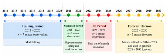
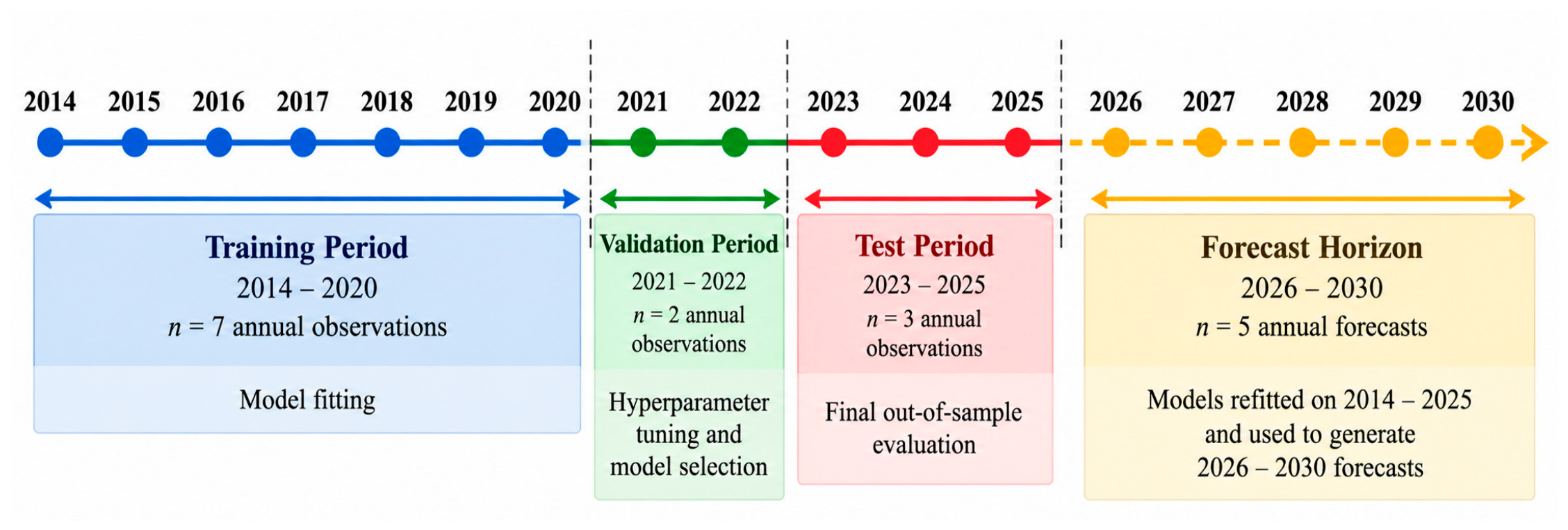
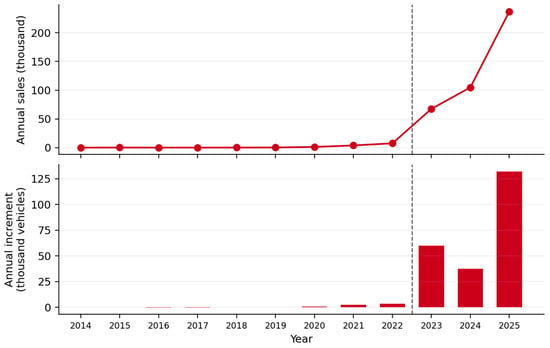
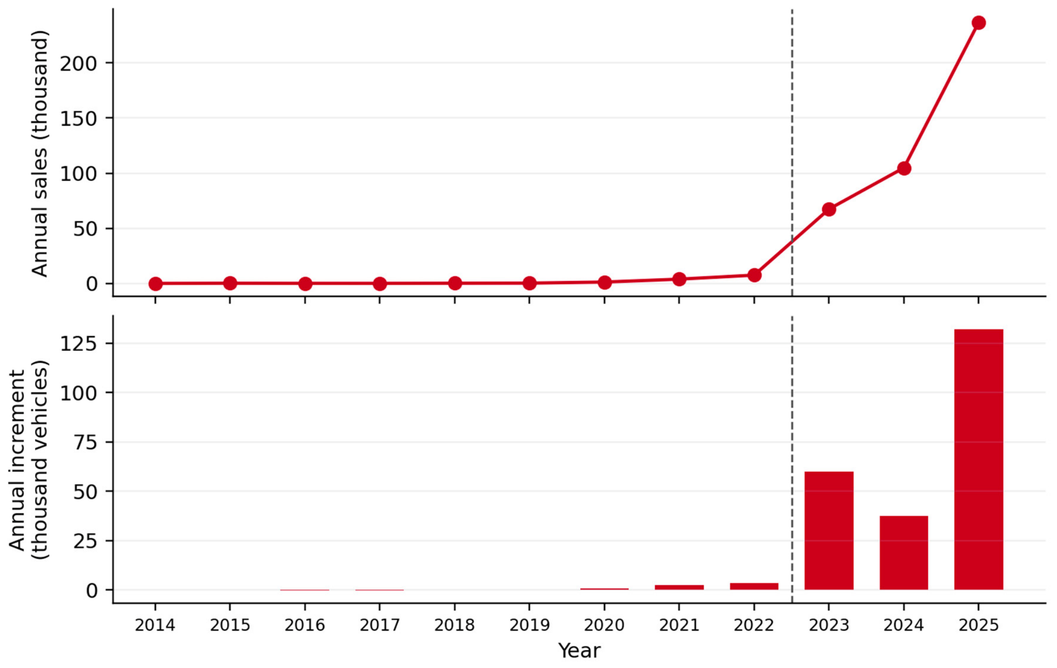
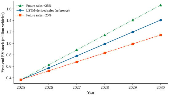
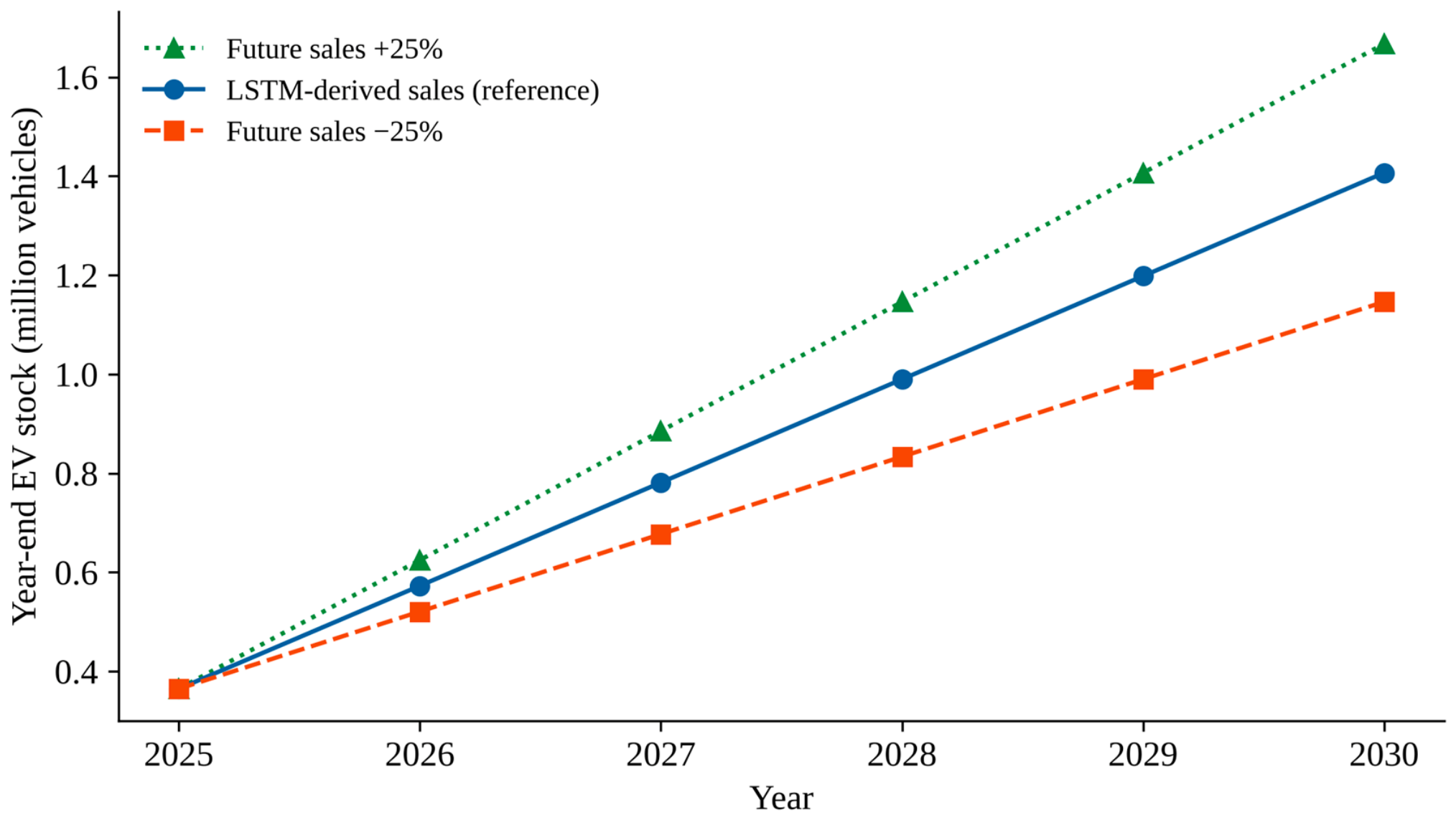
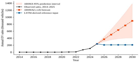
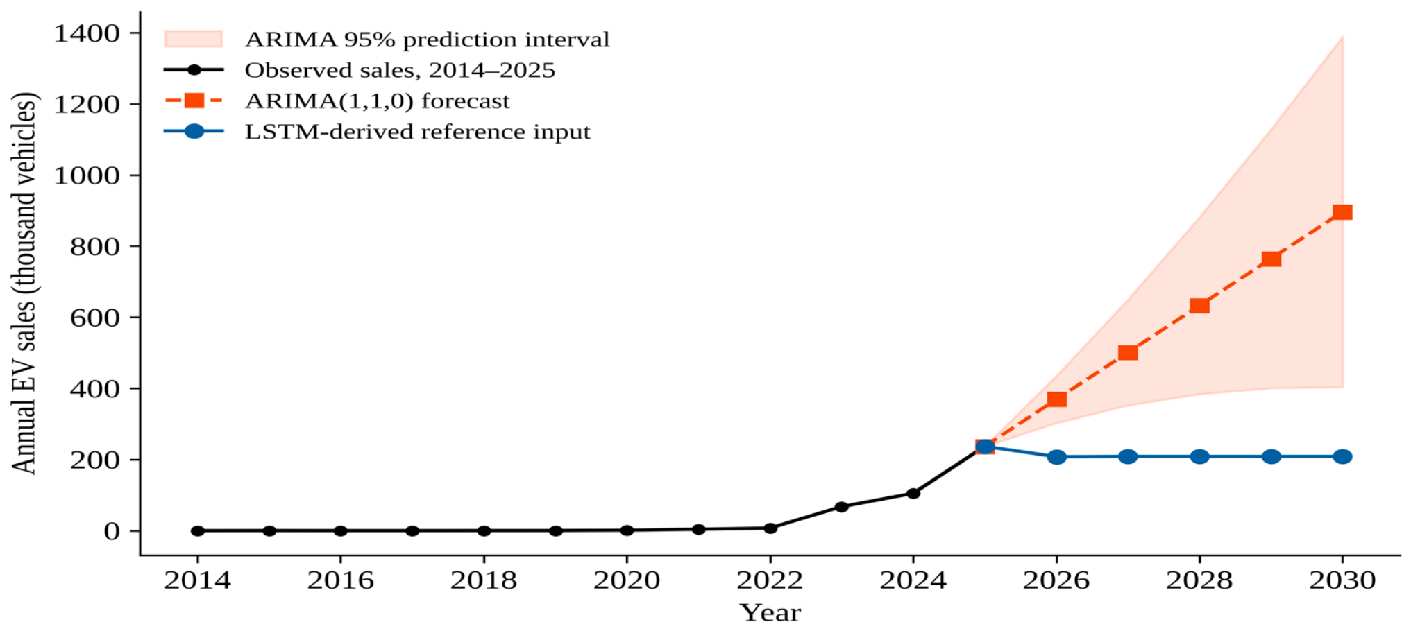
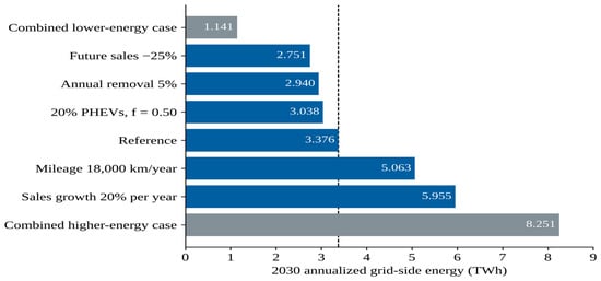
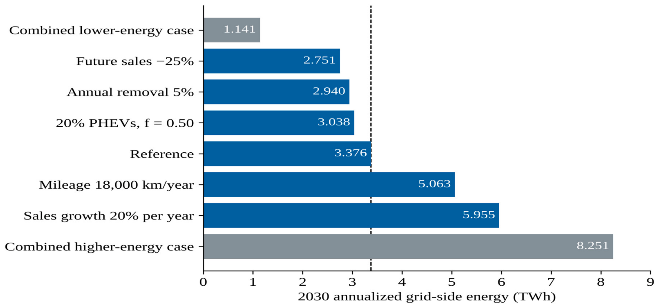

Disclaimer/Publisher’s Note: The statements, opinions and data contained in all publications are solely those of the individual author(s) and contributor(s) and not of MDPI and/or the editor(s). MDPI and/or the editor(s) disclaim responsibility for any injury to people or property resulting from any ideas, methods, instructions or products referred to in the content. |
© 2026 by the authors. Licensee MDPI, Basel, Switzerland. This article is an open access article distributed under the terms and conditions of the Creative Commons Attribution (CC BY) license.