An Empirical Study of Exhaustive Matching for Improving Motion Field Estimation

Abstract

Optical flow is defined as the motion field of pixels between two consecutive images. Traditionally, in order to estimate pixel motion field (or optical flow), an energy model is proposed. This energy model is composed of (i) a data term and (ii) a regularization term. The data term is an optical flow error estimation and the regularization term imposes spatial smoothness. Traditional variational models use a linearization in the data term. This linearized version of data term fails when the displacement of the object is larger than its own size. Recently, the precision of the optical flow method has been increased due to the use of additional information, obtained from correspondences computed between two images obtained by different methods such as SIFT, deep-matching, and exhaustive search. This work presents an empirical study in order to evaluate different strategies for locating exhaustive correspondences improving flow estimation. We considered a different location for matching random locations, uniform locations, and locations on maximum gradient magnitude. Additionally, we tested the combination of large and medium gradients with uniform locations. We evaluated our methodology in the MPI-Sintel database, which represents the state-of-the-art evaluation databases. Our results in MPI-Sintel show that our proposal outperforms classical methods such as Horn-Schunk, TV-L1, and LDOF, and our method performs similar to MDP-Flow.

1. Introduction

The apparent movement of pixels in a sequence of images is called the optical flow. Optical flow estimation is one of the most challenging problems in computer vision, especially in real scenarios where large displacements and illumination changes occur. Optical flow has many applications, including autonomous flight of vehicles, insertion of objects on video, slow camera motion generation, and video compression.

In particular, in video compression, the optical flow helps to remove temporal data redundancy and therefore to attain high compression ratios. In video processing, optical flow estimation is used, e.g., for deblurring and noise suppression.

In order to estimate the flow field that represents the motion of pixels in two consecutive frames of a video sequence, most of the optical flow methods are grounded in the optical flow constraint. This constraint is based on the brightness constancy assumption, which states that the brightness or intensity of objects remains constant from frame to frame along the movement of objects.

Let us consider two consecutive image frames, $I_0$ (reference) and $I_1$ (target), of a video sequence, where $I_0,I_1:\mathrm{\Omega }\to \mathbb{R}$ where $\mathrm{\Omega }\subset {\mathbb{R}}^2$ is the image domain (which is assumed to be a rectangle in ${\mathbb{R}}^2$) and $u:\mathrm{\Omega }\to {\mathbb{R}}^2$, and $\mathbf{u}\left(\mathbf{x}\right)=(u_1\left(\mathbf{x}\right),u_2\left(\mathbf{x}\right))$ i.e., $u_1,u_2:\mathrm{\Omega }\to \mathbb{R}$. The aim is to estimate a 2D motion field $u\left(\mathbf{x}\right)$ the optical flow, such that the image points $I_0\left(\mathbf{x}\right)$ and $I_1(\mathbf{x}+\mathbf{u}\left(\mathbf{x}\right))$ are observations of the same physical scene point. In other words, the brightness constancy assumption writes

$$I_0\left(\mathbf{x}\right)=I_1(\mathbf{x}+\mathbf{u}\left(\mathbf{x}\right))$$

(1)

for x ∈ $\mathrm{\Omega }$. Let us assume that the displacement $u\left(\mathbf{x}\right)$ is small enough to be valid the following linearized version of the brightness constancy assumption:

$$I_0\left(x\right)=I_1\left(\mathbf{x}\right)+<\nabla I_1\left(\mathbf{x}\right)·\mathbf{u}\left(\mathbf{x}\right)>$$

(2)

where $<,>$ denotes scalar product, and $\nabla I_1$ denotes the gradient of $I_1$ with respect to the space coordinates x and y, respectively. This equation can be rewritten as

$${\partial }_t{I}_1+<\nabla I_1\left(x\right),\mathbf{u}\left(\mathbf{x}\right)>=0$$

(3)

where ${\partial }_t{I}_1$ denotes $I_1\left(\mathbf{x}\right)-I_0\left(\mathbf{x}\right)$. Equation (3) is usually called the optical flow equation or optical flow constraint.

The optical flow constraint expressed by Equation (3) is only suitable when the partial derivatives can be correctly approximated. This is the case when the motion field is small enough or images are very smooth. However, in the presence of large displacements, these conditions are not typically preserved, and it is common to replace it with a nonlinear formulation [1].

$$I_0\left(\mathbf{x}\right)-I_1(\mathbf{x}+\mathbf{u}\left(\mathbf{x}\right))=0$$

(4)

for $x\in \mathrm{\Omega }$.

Neither Equation (3) nor Equation (4) can be solved pointwise since the number of parameters (the two components $u_1\left(\mathbf{x}\right),u_2\left(\mathbf{x}\right)$ of $\mathbf{u}\left(\mathbf{x}\right)$) to be estimated is larger than the number of equations.

To challenge these problems, a variational approach could be used and compute the optical flow $\mathbf{u}$ by minimizing the following energy or error measure,

$$J\left(\mathbf{u}\right)={\int }_{\mathrm{\Omega }}{\left|I_0\left(\mathbf{x}\right)-I_1(\mathbf{x}+u\left(\mathbf{x}\right))\right|}^{2}d\mathbf{x}.$$

(5)

However, Equation (5) is an ill-posed problem, which is usually challenged by adding a regularity prior. Then, the regularization term added to the energy model allows for a definition of the structure of the motion field and ensures that the optical flow computation is well posed. Ref. [2] proposed adding a quadratic regularization term. This work was the first that introduced variational methods to compute dense optical flow. An optical flow $\mathbf{u}$ is estimated as the minimizer of the following energy functional

$$J\left(\mathbf{u}\left(\mathbf{x}\right)\right)={\int }_{\mathrm{\Omega }}{\left|I_0\left(\mathbf{x}\right)-I_1(\mathbf{x}+\mathbf{u}\left(\mathbf{x}\right))\right|}^{2}d\mathbf{x}+{\int }_{\mathrm{\Omega }}{\left|\nabla \mathbf{u}\left(\mathbf{x}\right)\right|}^{2}d\mathbf{x}$$

(6)

where $\nabla \mathbf{u}\left(\mathbf{x}\right)=(\nabla u_1\left(\mathbf{x}\right),\nabla u_2\left(\mathbf{x}\right))$ denotes the gradient of the optical flow. This $L^2$ regularity prior does not cope well with motion discontinuities and other regularization terms have been proposed [3,4,5]. Although the original work of Horn and Schunk reveals many limitations (e.g., the computed optical flow is very smooth and sensitive to the presence of noise), it has inspired many proposals. In order to cope with large displacements, optimization typically proceeds in a coarse-to-fine manner (also called a multi-scale strategy).

Let us now focus on the data term in (6), ${\displaystyle J_D\left(\mathbf{u}\left(\mathbf{x}\right)\right)={\int }_{\mathrm{\Omega }}{\left|I_0\left(\mathbf{x}\right)-I_1(\mathbf{x}+\mathbf{u}\left(\mathbf{x}\right))\right|}^{2}d\mathbf{x}}$. The brightness constancy constraint assumes that the illumination of the scene is constant over time and that the image brightness of a point remains constant along its motion trajectory. Therefore, changes in brightness are only due to different objects and different movements.

Let us briefly remark that a problem is called ill-posed if its solution either does not exist or it is not unique. We have observed that the optical flow Equation (3) (or (4)) is an ill-posed problem: it cannot be solved pointwise as there is a unique equation as well as two unknowns $u_1\left(\mathbf{x}\right)$ and $u_2\left(\mathbf{x}\right)$. The optical flow expressed by Equation (3) can be rewritten as

$$<\nabla I,\mathbf{u}\left(\mathbf{x}\right)>=-{\partial }_{t}I\left(\mathbf{x}\right)$$

(7)

where ${\partial }_{t}I$ is the temporal derivative of I, by considering a local orthonormal basis $\{e_1,e_2\}$ of ${\mathbb{R}}^2$ on directions of $\nabla I\left(\mathbf{x}\right)$ and $\nabla I{\left(\mathbf{x}\right)}^{\perp }$. The optical flow $\mathbf{u}\left(\mathbf{x}\right)$ can be expressed in this basis, $\mathbf{u}=u_p\left(\mathbf{x}\right)e_1+u_{\perp }\left(\mathbf{x}\right)e_2$, where $u_p\left(\mathbf{x}\right)e_1$ is the projection of $\mathbf{u}\left(\mathbf{x}\right)$ in the gradient direction and $u_{\perp }\left(\mathbf{x}\right)e_2$ is the projection of the optical flow $\mathbf{u}\left(\mathbf{x}\right)$ in the direction perpendicular to the gradient. Thus, Equation (7) can be formally written as

$$<\nabla I\left(\mathbf{x}\right),u_p\left(\mathbf{x}\right)e_1+u_{\perp }\left(\mathbf{x}\right)e_2>=\parallel \nabla I\left(\mathbf{x}\right)\parallel u_p\left(\mathbf{x}\right)=-{\partial }_{t}I\left(\mathbf{x}\right).$$

(8)

This equation can be solved for $u_p\left(\mathbf{x}\right)$, $u_p\left(\mathbf{x}\right)=-\frac{{\partial }_{t}I\left(\mathbf{x}\right)}{\parallel \nabla I\left(\mathbf{x}\right)\parallel }$, if $\parallel \nabla I\left(\mathbf{x}\right)\parallel \ne 0$. In other words, the only component of the optical flow that can be determined from Equation (3) is the component parallel to the gradient direction. This indeterminacy is called the aperture problem.

1.1. Optical Flow Estimation

The most accurate techniques that address the motion estimation problem are based on the formulation of the optical flow estimation in a variational setting. Energy-based methods are called global methods since they find correspondences by minimizing an energy defined on the whole image (such as inthe minimizing problem of Equation (6)). They provide a dense solution with subpixel accuracy and are usually called dense optical flow methods.

The authors in [2] estimate a dense optical flow field based on two assumptions: the brightness constancy assumption and a smooth spatial variation of the optical flow. They proposed the following functional:

$$J\left(u\right)={\int }_{\mathrm{\Omega }}{\left|{\partial }_{x}I{u}_1\left(\mathbf{x}\right)+{\partial }_{y}I{u}_2\left(\mathbf{x}\right)+{\partial }_{t}I\left(\mathbf{x}\right)\right|}^{2}d\mathbf{x}+{\alpha }^2{\int }_{\mathrm{\Omega }}{\left|\nabla u_1\left(\mathbf{x}\right)\right|}^2+{\left|\nabla u_2\left(\mathbf{x}\right)\right|}^{2}d\mathbf{x}$$

(9)

where $\alpha$ is a real parameter that controls the influence of the smooth term. This functional is convex and has a unique minimizer. However, the computed optical flow is very smooth and does not preserve discontinuities of the optical flow. This is also the case for Equation (6), which can be considered a variant of Equation (9).

After the initial work in [2], many approaches that focus on accuracy have been developed. These works focus on the use of robust estimators, either in the data or smoothness terms, to be able to deal with motion discontinuities generated by the movement of different objects or by occlusions (e.g., [5,6]). For the data term, $L^2$ or $L^1$ dissimilarity measures have been used as well as more advanced data terms [6]. For the smoothness term, isotropic diffusion, image-adaptive, isotropic diffusion with non-quadratic regularizers, anisotropic diffusion (image or flow-adaptive), and the recent non-local regularizers have been proposed [3,4,5,6].

However, these methods may fail in occlusion areas due to forced, but unreliable, intensity matching. The problem can be further accentuated if the optical flow is smoothed across an object boundaries adjacent to occlusion areas.

1.2. Robust Motion Estimation

Normally, assumptions as brightness constancy and smooth space variation of optical flow are violated in real images. Advanced robust optical flow methods are developed with the goal to perform well even when violations of the optical flow assumptions are present.

The model expressed by Equation (9) to estimate the optical flow penalizes high gradients of $\mathbf{u}\left(\mathbf{x}\right)$ and therefore does not allow discontinuities of $\mathbf{u}\left(\mathbf{x}\right)$. This model is highly sensitive to noise in the images and to outliers. The functional can be modified in order to allow discontinuities of the flow field by changing the quadratic data term to an $L^1$ term and by changing the $L^2$ regularization term. In [5], the authors present a novel approach to estimate the optical flow that preserves discontinuities, and it is robust to noise. In order to compute the optical flow $\mathbf{u}=(u_1,u_2):\mathrm{\Omega }\to {\mathbb{R}}^2$ between $I_0$ and $I_1$, the authors propose minimizing the energy:

$$J\left(\mathbf{u}\left(\mathbf{x}\right)\right)={\int }_{\mathrm{\Omega }}\left(\lambda \right|I_0\left(\mathbf{x}\right)-I_1(\mathbf{x}+\mathbf{u}\left(\mathbf{x}\right))|+|\nabla u_1\left(\mathbf{x}\right)|+|\nabla u_2\left(\mathbf{x}\right)\left|\right)d\mathbf{x},$$

(10)

including robust data attachment and regularization terms (namely, the total variation of $\mathbf{u}\left(\mathbf{x}\right)$) with a relative weight given by the parameter $\lambda >0$. This variational model is usually called the TV-L1 formulation. The use of $L^1$ type-norm measures has shown a good performance in front of $L^2$ norms to preserve discontinuities in the flow field and offers increased robustness against noise and illumination changes.

1.3. Related Works

As we mentioned above, motion estimation methods use an approximation of the data term. Energies that consider this approximation fail to estimate the optical flow when the displacements are very fast or larger than the size of the objects in the scene. Recently, a new term that considers correspondences between two images have been added to these kinds of models [3,6,7,8]. The inclusion of this additional information (as a prior) has improved the performance of the optical flow estimation, giving the model the capability of handle large displacements. The inclusion of this new term allows the methodology to be systematic and not depending on heuristic and complex rules that depend on the designer of the model.

In [3], the authors propose a model to handle large displacement. This model stated an energy model that considers (i) a data term, (ii) a regularization term, and (iii) a term for additional information. The additional information term proposed in this energy model comes from correspondences obtained either by SIFT or by patch match. Considering these computed correspondences, a constant candidate flow is proposed as a possible motion present in the image. Authors select the optimal flow among the constant candidates for each pixel in the image sequence as a labeling problem. The authors solve this problem using discrete optimization QPBO (quadratic pseudo-Boolean optimization).

In [9], a model is presented for estimating the optical flow that utilizes a robust data term, a regularization term, and a term that considers additional matching. Additional matching is obtained using HoGs (Histograms of Gradients). The incorporation of additional matching is weighted by a confidence value that is not simple to compute. This weight depends on the distance to the second best candidate of the matching and on the ratio between the error of current optical flow estimation and the error of the new correspondence. The location of the matching depends on the minimum eigenvalue of the structure tensor of the image and on the error of the optical flow estimation.

Deep-flow presented in [10] is a motion field estimation method inspired by (i) deep convolution neural networks and (ii) the work of [6]. Deep flow is an optical flow estimation method to handle large displacements, which obtains dense correspondences between two consecutive images. These correspondences are obtained using small patches (of $4\times 4$ pixels). A patch of $8\times 8$ is interpreted as composed by 4 patches of $4\times 4$ pixels, each small patch is called a quadrant. The matching score of an $8\times 8$ patch is formed by averaging the max-pooled scores of the quadrants [10]. This process is repeated recursively for $16\times 16$, $32\times 32$, and $64\times 64$ pixels becoming a more discriminant virtual patch. Computed matching is considered a prior term in an energy model. Deep flow uses a uniform grid to locate the correspondences. A study in depth is necessary for this proposed method. Which patch size is necessary to improve the results and which locations are the best to improve optical flow estimation are questions that must be answered.

Recently, new models have been proposed in order to tackle the problem of large displacements in [4,11,12,13]. These models consider sparse or dense matching using a deep matching algorithm [10], motion candidates [13], or SIFT. The principle idea is to give some “hint” to the variational optical flow approach by using such sparse matching [10]. In [12,13], an occlusion layer is also estimated.

In [11], the authors propose a method called SparseFlow that finds sparse pixel correspondences by mean of a matching algorithm, and these correspondences are used to guide a variational approach to obtain a refined optical flow. The SparseFlow matching algorithm uses an efficient sparse decomposition of pixels surrounding a patch as a linear sum of those found around candidate corresponding pixels [11]. The matching pixel dominating the decomposition is chosen. The pixel pair matching in both directions (forward–backward) are used to refine the optical flow estimation.

In [12], a successful method to compute optical flow is proposed which includes occlusion handling and additional temporal information. Images are divided into discrete triangles, and this allowed the authors to naturally estimate the occlusions that are then incorporated into the optimization algorithm to estimate an optical flow. Combining the “Inertial Estimate” of the flow and classifiers to fusion optical flow, they made some improvements in the final results.

The authors in [13] propose a method to compute motion field, and this method aims to tackle large displacements, motion detail, and occlusion estimation. The method consists of two stages: (i) They supply dense local motion candidates. (ii) They estimate affine motion models over a set of size-varying patches combined with a patch-based pairing.

In [14], an optical flow method that includes this new term for additional information coming from exhaustive matching is proposed. This model also considers an occlusion layer simultaneously estimated with optical flow. The estimation of the occlusion layer helps to improve the motion estimation of regions that are visible in the current frame but not visible in the next frame.

In this work, we present an empirical study to evaluate different strategies to locate additional exhaustive matching (correspondences coming from exhaustive search) in order to improve the precision of the motion field or optical flow estimation. We think that none of the above-revised works has answered precisely the question “What is the best location for additional correspondences in order to improve the precision of a motion estimation method?” We considered three possible locations of matching: (i) uniform locations, (ii) random locations, and (iii) locations in the maximum gradient of the reference frame. We also evaluated combined strategies: uniform locations in large gradients magnitude and uniform locations located in medium gradients magnitude. We performed two evaluations using different features. In the first one we used intensities, and in the second, we used gradients.

We present our complete evaluation strategy in Section 5.

1.4. Contribution of This Version

In this new version of the paper presented in [15], we have implemented the following modifications:

(a)

We determine the parameters of the optical flow estimation model using particle swarm optimization (PSO).

(b)

Our proposal was evaluated in the large database MIP-Sintel in both of its sets: training and test.

(c)

We estimated the occluded pixels in two consecutive images based on the largest values of the optical flow error. We avoided computing exhaustive matching in these occluded pixels because the matching will be unreliable.

(d)

We divided the gradient of the image into three sets: (i) small gradients, (ii) medium gradients, and (iii) large gradients. In sets (ii) and (iii), we have located additional matching in uniform locations and we have evaluated the performance in MPI-Sintel.

(e)

We extended the Horn-Schunck optical flow to handle additional information coming from exhaustive search. This extended method was evaluated in the MPI-Sintel Database, and the obtained results were compared with the results obtained by our proposal.

(f)

We performed exhaustive matching using colors and using gradients in order to make this experimental study more complete.

In Section 2, we present our proposal to estimate the motion field. In Section 3, the implementation of the methods is presented and we present the pseudo-code of the algorithm. In Section 4.3, we present the experiments and the database used, and in Section 5 the obtained results are presented. We present comments and discussions about the obtained results in Section 6.

2. Materials and Methods

We present in Section 2.1 our proposed model to handle large displacements and be robust to illumination changes. In Section 2.3 we extended the classical Horn-Shunck method to handle large displacement. Our aim is to compare the effect of using additional term in our proposed model and in the Horn-Shunck model.

2.1. Proposed Model

Models presented in [3,5,7,16] propose a variational model to estimate the motion field. Those cited models use the $L^1$ norm (a data term which is robust to illumination changes and tolerate discontinuities) and an additional term that incorporates information coming from a correspondences estimation method.

Let $I_0$ and $I_1$ be two consecutive images and let $\mathbf{u}=(u_1,u_2)$ be the motion field between images such that

$$J\left(\mathbf{u}\left(\mathbf{x}\right)\right)=J_d\left(\mathbf{u}\left(\mathbf{x}\right)\right)+J_r\left(\mathbf{u}\left(\mathbf{x}\right)\right)$$

where $\mathrm{\Omega }\subset {\mathbb{R}}^2$, and $J_d\left(\mathbf{u}\left(\mathbf{x}\right)\right)$ is the data term and is given by

$$J_d\left(\mathbf{u}\left(\mathbf{x}\right)\right)={\int }_{\mathrm{\Omega }}\lambda \left|I_0\left(\mathbf{x}\right)-I_1(\mathbf{x}+\mathbf{u})\right|d\mathbf{x}.$$

(11)

where $\lambda$ is a real constant, and the regularization term $J_r\left(\mathbf{u}\left(\mathbf{x}\right)\right)$ is given by

$${\displaystyle J_r\left(\mathbf{u}\left(\mathbf{x}\right)\right)={\int }_{\mathrm{\Omega }}\sqrt{{\left|\nabla u_1\left(\mathbf{x}\right)\right|}^2+{\left|\nabla u_2\left(\mathbf{x}\right)\right|}^2}d\mathbf{x}.}$$

2.2. Linearization

The model presented in [5] considers a linearization of the data term in Equation (11). $I_1(\mathbf{x}+\mathbf{u}\left(\mathbf{x}\right))$ is linearized around a known point ${\mathbf{u}}_{\mathbf{0}}\left(\mathbf{x}\right)$ as

$$I_1(\mathbf{x}+\mathbf{u}\left(\mathbf{x}\right))=I_1(\mathbf{x}+{\mathbf{u}}_{\mathbf{0}}\left(\mathbf{x}\right))+<\mathbf{u}\left(\mathbf{x}\right)-{\mathbf{u}}_{\mathbf{0}},\nabla I_1(\mathbf{x}+{\mathbf{u}}_{\mathbf{0}}\left(\mathbf{x}\right))>$$

where ${\mathbf{u}}_{\mathbf{0}}\left(\mathbf{x}\right)$ is a known optical flow, $\nabla I_1(\mathbf{x}+{\mathbf{u}}_{\mathbf{0}}\left(\mathbf{x}\right))$ is the gradient of the warped image $I_1(\mathbf{x}+{\mathbf{u}}_{\mathbf{0}}\left(\mathbf{x}\right))$, and the notation $<,>$ represents the internal product. Considering this linearization, we obtain a new data term that can be written as

$${\tilde{J}}_d\left(\mathbf{u}\left(\mathbf{x}\right)\right)={\int }_{\mathrm{\Omega }}\lambda |I_1(\mathbf{x}+{\mathbf{u}}_{\mathbf{0}}\left(\mathbf{x}\right))+<\mathbf{u}\left(\mathbf{x}\right)-{\mathbf{u}}_{\mathbf{0}}\left(\mathbf{x}\right),\nabla I_1(\mathbf{x}+{\mathbf{u}}_{\mathbf{0}}\left(\mathbf{x}\right))>-I_0\left(\mathbf{x}\right)|d\mathbf{x}.$$

(12)

The data term in Equation (12) is based on the brightness constancy assumption, which states that the intensity of the pixels in the image remains constant along the sequence. In most cases, this assumption does not hold due to shadows, reflections, or illumination changes. The presence of shadows and other intensity changes cause the brightness constancy assumption to fail. The gradient constancy assumption appears as an alternative that can handle pixel intensity changes.

We define a weight map $\alpha :{\mathbb{R}}^2\to [0,1]$ to switch between the brightness and gradient constancy assumption as in [3]. We construct a new data term:

$$J_d\left(\mathbf{u}\left(\mathbf{x}\right)\right)=\lambda {\int }_{\mathrm{\Omega }}\alpha \left(\mathbf{x}\right)D_I(\mathbf{u}\left(\mathbf{x}\right),\mathbf{x})d\mathbf{x}+\lambda {\int }_{\mathrm{\Omega }}{\tau }_d(1-\alpha \left(\mathbf{x}\right))D_{\nabla I}(\mathbf{u}\left(\mathbf{x}\right),\mathbf{x})d\mathbf{x}$$

(13)

where

$$D_I(\mathbf{u}\left(\mathbf{x}\right),\mathbf{x})=|I_1(\mathbf{x}+{\mathbf{u}}_{\mathbf{0}}\left(\mathbf{x}\right))+<\mathbf{u}\left(\mathbf{x}\right)-{\mathbf{u}}_{\mathbf{0}}\left(\mathbf{x}\right),\nabla I_1(\mathbf{x}+{\mathbf{u}}_{\mathbf{0}}\left(\mathbf{x}\right))>-I_0\left(\mathbf{x}\right)|.$$

(14)

Equation (14) represents a linearized version of the brightness constancy assumption, and

$$\begin{array}{c}\hfill D_{\nabla I}(\mathbf{u}\left(\mathbf{x}\right),\mathbf{x})=|{\partial }_x{I}_1(\mathbf{x}+{\mathbf{u}}_{\mathbf{0}}\left(\mathbf{x}\right))+<\mathbf{u}\left(\mathbf{x}\right)-{\mathbf{u}}_{\mathbf{0}}\left(\mathbf{x}\right),\nabla {\partial }_x{I}_1(\mathbf{x}+{\mathbf{u}}_{\mathbf{0}}\left(\mathbf{x}\right))>-{\partial }_x{I}_0\left(\mathbf{x}\right)|\\ \hfill +|{\partial }_y{I}_1(\mathbf{x}+{\mathbf{u}}_{\mathbf{0}}\left(\mathbf{x}\right))+<\mathbf{u}\left(\mathbf{x}\right)-{\mathbf{u}}_{\mathbf{0}}\left(\mathbf{x}\right),\nabla {\partial }_y{I}_1(\mathbf{x}+{\mathbf{u}}_{\mathbf{0}}\left(\mathbf{x}\right))>& -{\partial }_y{I}_0\left(\mathbf{x}\right)|\hfill \end{array}$$

(15)

represents the gradient constancy assumption, where ${\tau }_d$ is a positive constant. In Equation (15), the terms ${\partial }_x{I}_0$, ${\partial }_x{I}_1$, and ${\partial }_y{I}_0$, ${\partial }_y{I}_1$ are the partial derivatives w.r.t. x and y of $I_0$ and $I_1$, respectively. Considering Equations (14) and (15), we follow [3] and state the adaptive weight map $\alpha \left(x\right)$:

$$\alpha \left(\mathbf{x}\right)=\frac{1}{1+e^{\beta (D_I(\mathbf{u}\left(\mathbf{x}\right),\mathbf{x})-{\tau }_d{D}_{\nabla I}(\mathbf{u}\left(\mathbf{x}\right),\mathbf{x}))}}$$

where $\beta$ is a positive constant real value.

Computing $\alpha \left(\mathbf{x}\right)$ depends on the difference of two terms: $D_I(\mathbf{u}\left(\mathbf{x}\right),\mathbf{x})$ and $D_{\nabla }(\mathbf{u}\left(\mathbf{x}\right),\mathbf{x})$. On the one hand, if $D_I(\mathbf{u}\left(\mathbf{x}\right),\mathbf{x})$ is larger than $D_{\nabla }(\mathbf{u}\left(\mathbf{x}\right),\mathbf{x})$, the data term will be more confident w.r.t. the gradient constancy constraint. On the other hand, if $D_I(\mathbf{u}\left(\mathbf{x}\right),\mathbf{x})$ is less than $D_{\nabla }(\mathbf{u}\left(\mathbf{x}\right),\mathbf{x})$, the data term will be more confident w.r.t. the color constancy constraint [3,8].

2.2.1. Decoupling Variable

In order to minimize the proposed functional in Equation (11), we propose using three decoupling variables (${\mathbf{v}}_{\mathbf{1}}\left(\mathbf{x}\right)$, ${\mathbf{v}}_{\mathbf{2}}\left(\mathbf{x}\right)$, ${\mathbf{v}}_{\mathbf{3}}\left(\mathbf{x}\right)$), and we penalize its deviation from $\mathbf{u}\left(\mathbf{x}\right)$, then the functional becomes

$$\begin{array}{cc}\hfill J(\mathbf{u}\left(\mathbf{x}\right),{\mathbf{v}}_{\mathbf{1}}\left(\mathbf{x}\right),{\mathbf{v}}_{\mathbf{2}}\left(\mathbf{x}\right),{\mathbf{v}}_{\mathbf{3}}\left(\mathbf{x}\right))& =J_d(\mathbf{u}\left(\mathbf{x}\right),{\mathbf{v}}_{\mathbf{1}}\left(\mathbf{x}\right),{\mathbf{v}}_{\mathbf{2}}\left(\mathbf{x}\right),{\mathbf{v}}_{\mathbf{3}}\left(\mathbf{x}\right))+J_r\left(\mathbf{u}\left(\mathbf{x}\right)\right)\hfill \\ \hfill +& \frac{1}{2\theta }{\int }_{\mathrm{\Omega }}\sum _{i=1}^3{\overline{\alpha }}_i{(\mathbf{u}\left(\mathbf{x}\right)-{\mathbf{v}}_{\mathbf{i}}\left(\mathbf{x}\right))}^{2}d\mathbf{x}\hfill \end{array}$$

(16)

where $\overline{\alpha }$ is a vector in ${\mathbb{R}}^3$ and is defined as $\overline{\alpha }\left(\mathbf{x}\right)={\left(\alpha \left(\mathbf{x}\right),1-\alpha \left(\mathbf{x}\right), \mathit{and} 1-\alpha \left(\mathbf{x}\right)\right)}^T$.

2.2.2. Color Model

Considering color images in RGB space ($I=\{I_1,I_2,I_3\}$, which correspond to red, blue, and green components, respectively), we define five decoupling variables ${\mathbf{v}}_{\mathbf{1}}\left(\mathbf{x}\right)$, ${\mathbf{v}}_{\mathbf{2}}\left(\mathbf{x}\right)$, and ${\mathbf{v}}_{\mathbf{3}}\left(\mathbf{x}\right)$ for color components and ${\mathbf{v}}_{\mathbf{4}}\left(\mathbf{x}\right)$ and ${\mathbf{v}}_{\mathbf{5}}\left(\mathbf{x}\right)$ for gradients; thus, the functional becomes

$$J(\mathbf{u}\left(\mathbf{x}\right),\overline{\mathbf{v}}\left(\mathbf{x}\right))=J_d(\mathbf{u}\left(\mathbf{x}\right),\overline{\mathbf{v}}\left(\mathbf{x}\right))+J_r\left(\mathbf{u}\left(\mathbf{x}\right)\right)+\frac{1}{2\theta }{\int }_{\mathrm{\Omega }}\sum _{i=1}^5{\overline{\alpha }}_i\left(\mathbf{x}\right){(\mathbf{u}\left(\mathbf{x}\right)-{\mathbf{v}}_{\mathbf{i}}\left(\mathbf{x}\right))}^{2}d\mathbf{x}$$

(17)

where we have defined $\overline{\mathbf{v}}\left(\mathbf{x}\right)=\{{\mathbf{v}}_{\mathbf{1}}\left(\mathbf{x}\right),{\mathbf{v}}_{\mathbf{2}}\left(\mathbf{x}\right),{\mathbf{v}}_{\mathbf{3}}\left(\mathbf{x}\right),{\mathbf{v}}_{\mathbf{4}}\left(\mathbf{x}\right), \mathrm{and} {\mathbf{v}}_{\mathbf{5}}\left(\mathbf{x}\right)\}$, and $\overline{\alpha }\in {\mathbb{R}}^5$ is defined as $\overline{\alpha }\left(\mathbf{x}\right)={\left(\alpha \left(\mathbf{x}\right),\alpha \left(\mathbf{x}\right),\alpha \left(\mathbf{x}\right),1-\alpha \left(\mathbf{x}\right),and 1-\alpha \left(\mathbf{x}\right)\right)}^T$.

2.2.3. Optical Flow to Handle Large Displacements

In order to cope with large displacements, we use additional information coming from exhaustive matching computed between images of a video sequence used as a precomputed sparse vector field (a priori). The main idea is that this sparse vector field guides the optical flow estimation in regions where the approximated linearized model fails [7] due to fast movements or large displacements.

Let ${\mathbf{u}}_{\mathbf{e}}\left(\mathbf{x}\right)$ be this sparse vector field. We add to our model a term to enforce the solution $\mathbf{u}\left(\mathbf{x}\right)$ to be similar to the sparse flow ${\mathbf{u}}_{\mathbf{e}}\left(\mathbf{x}\right)$ as in [7], and our model becomes

$$\begin{array}{cc}\hfill J(\mathbf{u}\left(\mathbf{x}\right),\overline{\mathbf{v}}\left(\mathbf{x}\right),{\mathbf{u}}_{\mathbf{e}}\left(\mathbf{x}\right))=& {\tilde{J}}_d(\mathbf{u}\left(\mathbf{x}\right),\overline{\mathbf{v}}\left(\mathbf{x}\right))+J_r\left(\mathbf{u}\left(\mathbf{x}\right)\right)+\frac{1}{2\theta }{\int }_{\mathrm{\Omega }}\sum _{i=1}^5{\overline{\alpha }}_i{(\mathbf{u}\left(\mathbf{x}\right)-{\mathbf{v}}_{\mathbf{i}}\left(\mathbf{x}\right))}^{2}d\mathbf{x}\hfill \\ & +{\int }_{\mathrm{\Omega }}\kappa \chi \left(\mathbf{x}\right){(\mathbf{u}\left(\mathbf{x}\right)-{\mathbf{u}}_{\mathbf{e}}\left(\mathbf{x}\right))}^{2}d\mathbf{x}\hfill \end{array}$$

where $\chi \left(\mathbf{x}\right)$ is a binary mask indicating where the matching was computed. $\kappa$ is a decreasing weight for each scale. Following [7], the $\kappa$ is updated for each iteration $\kappa ={\kappa }_0{\left(0.5\right)}^n$, where ${\kappa }_0=300$, and n is the iteration number.

We use this $\chi \left(\mathbf{x}\right)$ binary mask to test different locations of ${\mathbf{u}}_{\mathbf{e}}\left(\mathbf{x}\right)$ in order to evaluate its influence in the optical flow estimation performance.

2.2.4. Occlusion Estimation

The proposed model cannot handle occluded and dis-occluded pixel. There is no correspondence for pixels that are visible in the current frame and not visible in the target frame. Optical flow computed in those pixels presents a large error due to the forced matching. We used this fact to detect an occlusion and once the occlusion is detected we do not perform exhaustive matching in those points. That is to say, we define regions where the exhaustive matching must not be performed. As a proof of concept, we show in Figure 1 two consecutive frames of the sequence ambush_5 where the girl fights with a man. The sequence presents large regions where pixels are occluded.

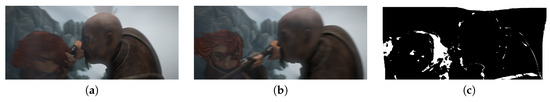
Figure 1. Occlusion estimation comparing optical flow error with a threshold ${\theta }_{occ}$. (a) Frame_0049 of sequence ambush_5; (b) Frame_0050; (c) occlusion estimation.

We present in Figure 1 two consecutive images in (a) and (b), and in (c) we present our occlusion estimation. In the sequence, the hair of the girl moves to the left of the image and the occlusion is correctly estimated. Additionally, dis-occlusion is estimated as we see on the right side of the girl’s head where hair dis-occluded the hand and the lance.

We compare the magnitude of the data term with a threshold (${\theta }_{occ}$) as in [17]. On the one hand, if the magnitude is larger than the threshold, then a binary mask $\mathbf{o}\left(x\right)$ is set to 1. On the other hand, if the magnitude is smaller than the threshold, $\mathbf{o}\left(\mathbf{x}\right)$ is set to 0.

2.2.5. Solving the Model

For a fixed ${\mathbf{u}}_{\mathbf{0}}\left(\mathbf{x}\right)$ and following the notation in [5] we define ${\rho }_i\left(\mathbf{u}\left(\mathbf{x}\right)\right)$. Let ${\rho }_i\left(\mathbf{u}\left(\mathbf{x}\right)\right)=I_i(\mathbf{x}+{\mathbf{u}}_{\mathbf{0}}\left(\mathbf{x}\right))+⟨\mathbf{u}\left(\mathbf{x}\right)-{\mathbf{u}}_{\mathbf{0}}\left(\mathbf{x}\right),\nabla I_i⟩-I_0$ with $i=1,\dots ,3$. ${\rho }_4\left(\mathbf{u}\left(\mathbf{x}\right)\right)={\partial }_x{I}_1(\mathbf{x}+{\mathbf{u}}_{\mathbf{0}}\left(\mathbf{x}\right))+⟨\mathbf{u}\left(\mathbf{x}\right)-{\mathbf{u}}_{\mathbf{0}}\left(\mathbf{x}\right),\nabla {\partial }_x{I}_1⟩-{\partial }_x{I}_0$ and ${\rho }_5\left(\mathbf{u}\left(\mathbf{x}\right)\right)={\partial }_y{I}_1(\mathbf{x}+{\mathbf{u}}_{\mathbf{0}}\left(\mathbf{x}\right))+⟨\mathbf{u}\left(\mathbf{x}\right)-{\mathbf{u}}_{\mathbf{0}}\left(\mathbf{x}\right),\nabla {\partial }_y{I}_1⟩-{\partial }_y{I}_0$. If $\theta$ is a small constant, then ${\mathbf{v}}_{\mathbf{1}}\left(\mathbf{x}\right)$, ${\mathbf{v}}_{\mathbf{2}}\left(\mathbf{x}\right)$, ${\mathbf{v}}_{\mathbf{3}}\left(\mathbf{x}\right)$, ${\mathbf{v}}_{\mathbf{4}}\left(\mathbf{x}\right)$, and ${\mathbf{v}}_{\mathbf{5}}\left(\mathbf{x}\right)$ are close to $\mathbf{u}\left(\mathbf{x}\right)$. This convex problem can be minimized by alternating steps as in [5]:

(1)

Solve exhaustively

$$J_d\left({\mathbf{u}}_{\mathbf{e}}\left(\mathbf{x}\right)\right)=\underset{{\mathbf{u}}_{\mathbf{e}}\left(\mathbf{x}\right)}{\min }{\int }_{\mathrm{\Omega }}\left|I_0\left(\mathbf{x}\right)-I_1(\mathbf{x}+{\mathbf{u}}_{\mathbf{e}}\left(\mathbf{x}\right))\right|d\mathbf{x}.$$

(18)

(2)

Let us fix ${\mathbf{v}}_{\mathbf{1}}\left(\mathbf{x}\right)$, ${\mathbf{v}}_{\mathbf{2}}\left(\mathbf{x}\right)$, ${\mathbf{v}}_{\mathbf{3}}\left(\mathbf{x}\right)$, ${\mathbf{v}}_{\mathbf{4}}\left(\mathbf{x}\right)$, and ${\mathbf{v}}_{\mathbf{5}}\left(\mathbf{x}\right)$ and then solve for $\mathbf{u}\left(\mathbf{x}\right)$:

$$\underset{\mathbf{u}\left(\mathbf{x}\right)}{\min }\left\{{\int }_{\mathrm{\Omega }}\sum _{i=1}^5\frac{{\overline{\alpha }}_i\left(\mathbf{x}\right){(\mathbf{u}\left(\mathbf{x}\right)-{\mathbf{v}}_{\mathbf{i}}\left(\mathbf{x}\right))}^2}{2\theta }d\mathbf{x}+{\int }_{\mathrm{\Omega }}\kappa \chi \left(\mathbf{x}\right)(1-\mathbf{o}\left(\mathbf{x}\right))(\mathbf{u}\left(\mathbf{x}\right)-{\mathbf{u}}_{\mathbf{e}}\left(\mathbf{x}\right))d\mathbf{x}+{\int }_{\mathrm{\Omega }}\parallel \nabla u\parallel d\mathbf{x}.\right\}$$

(19)

(3)

Let us fix $\mathbf{u}\left(\mathbf{x}\right)$ and solve the problem for ${\mathbf{v}}_{\mathbf{1}}\left(\mathbf{x}\right)$, ${\mathbf{v}}_{\mathbf{2}}\left(\mathbf{x}\right)$, ${\mathbf{v}}_{\mathbf{3}}\left(\mathbf{x}\right)$, ${\mathbf{v}}_{\mathbf{4}}\left(\mathbf{x}\right)$, and ${\mathbf{v}}_{\mathbf{5}}\left(\mathbf{x}\right)$:

$$\underset{{\mathbf{v}}_{\mathbf{i}}\left(\mathbf{x}\right)}{\min }\left\{{\int }_{\mathrm{\Omega }}\sum _{i=1}^5{(\mathbf{u}\left(\mathbf{x}\right)-{\mathbf{v}}_{\mathbf{i}}\left(\mathbf{x}\right))}^{2}d\mathbf{x}+{\int }_{\mathrm{\Omega }}\left|{\rho }_i\left({\mathbf{v}}_{\mathbf{i}}\left(\mathbf{x}\right)\right)\right|d\mathbf{x}.\right\}.$$

(20)

This minimization problem for ${\mathbf{v}}_{\mathbf{1}}\left(\mathbf{x}\right)$${\mathbf{v}}_{\mathbf{2}}\left(\mathbf{x}\right)$, ${\mathbf{v}}_{\mathbf{3}}\left(\mathbf{x}\right)$, ${\mathbf{v}}_{\mathbf{4}}\left(\mathbf{x}\right)$, and ${\mathbf{v}}_{\mathbf{5}}\left(\mathbf{x}\right)$ can be solved point-wise. Since the propositions in [5] are fundamentals for our work, we adapted them to our model.

Proposition 1.

The solution of Equation (9) is given by

$$u\left(\mathbf{x}\right)=\frac{\alpha \left(\mathbf{x}\right)\left(\frac{{\mathbf{v}}_{\mathbf{1}}\left(\mathbf{x}\right)+{\mathbf{v}}_{\mathbf{2}}\left(\mathbf{x}\right)+\mathbf{v}\mathbf{3}\left(\mathbf{x}\right)}{3}\right)+(1-\alpha \left(\mathbf{x}\right))\left(\frac{{\mathbf{v}}_{\mathbf{4}}\left(\mathbf{x}\right)+{\mathbf{v}}_{\mathbf{5}}\left(\mathbf{x}\right)}{2}\right)+\theta div\left(g\left(\mathbf{x}\right)\xi \left(\mathbf{x}\right)\right)+\kappa \chi \left(\mathbf{x}\right)(1-\mathbf{o}\left(\mathbf{x}\right)){\mathbf{u}}_{\mathbf{e}}\left(\mathbf{x}\right)}{1+\kappa \chi \left(\mathbf{x}\right)(1-\mathbf{o}(\mathbf{x}\left)\right)}$$

(21)

The dual variable $\xi \left(\mathbf{x}\right)={({\xi }_1\left(\mathbf{x}\right),{\xi }_2\left(\mathbf{x}\right))}^T$ is defined as

$${\xi }_1\left(\mathbf{x}\right)=\frac{{\xi }_1\left(\mathbf{x}\right)+\frac{\tau }{\theta }\nabla u_1\left(\mathbf{x}\right)}{1+\frac{\tau }{\theta }\sqrt{|\nabla u_1{\left(\mathbf{x}\right)|}^2+{|\nabla u_2\left(\mathbf{x}\right)|}^2}}$$

(22)

$${\xi }_2\left(\mathbf{x}\right)=\frac{{\xi }_2\left(\mathbf{x}\right)+\frac{\tau }{\theta }\nabla u_2\left(\mathbf{x}\right)}{1+\frac{\tau }{\theta }\sqrt{|\nabla u_1{\left(\mathbf{x}\right)|}^2+{|\nabla u_2\left(\mathbf{x}\right)|}^2}}$$

(23)

where $\tau <\frac{1}{4}$.

Proposition 2.

The solution of the minimizing problem in Equation (20) is given by

$${\mathbf{v}}_{\mathbf{i}}\left(\mathbf{x}\right)=\mathbf{u}\left(\mathbf{x}\right)+\left\{\begin{array}{c}3\lambda \theta \nabla I_i(\mathbf{x}+{\mathbf{u}}_0\left(\mathbf{x}\right))\mathrm{if}{\rho }_i\left(\mathbf{u}\left(\mathbf{x}\right)\right)<-3\lambda \theta {|\nabla I_i(\mathbf{x}+{\mathbf{u}}_0\left(\mathbf{x}\right))|}^2\hfill \\ -\frac{{\rho }_i\left(\mathbf{u}\left(\mathbf{x}\right)\right)}{|\nabla I_i|}\nabla I_i(\mathbf{x}+{\mathbf{u}}_0\left(\mathbf{x}\right))\mathrm{if}|{\rho }_i\left(\mathbf{u}\left(\mathbf{x}\right)\right)|<3\lambda \theta |\nabla I_i(\mathbf{x}+{\mathbf{u}}_0\left(\mathbf{x}\right)){|}^2\\ -3\lambda \theta \nabla I_i(\mathbf{x}+{\mathbf{u}}_0\left(\mathbf{x}\right))\mathrm{if}{\rho }_i\left(\mathbf{u}\left(\mathbf{x}\right)\right)>3\lambda \theta {|\nabla I_i(\mathbf{x}+{\mathbf{u}}_0\left(\mathbf{x}\right))|}^2\end{array}\right.$$

(24)

$${\mathbf{v}}_{\mathbf{i}}\left(\mathbf{x}\right)=\mathbf{u}\left(\mathbf{x}\right)+\left\{\begin{array}{c}2\lambda \theta {\tau }_d\nabla {\partial }_i{I}_1(\mathbf{x}+{\mathbf{u}}_0\left(\mathbf{x}\right))\mathrm{if}{\rho }_i\left(\mathbf{u}\left(\mathbf{x}\right)\right)<-2\lambda \theta {\tau }_d{|\nabla {\partial }_i{I}_1(\mathbf{x}+{\mathbf{u}}_0\left(\mathbf{x}\right))|}^2\hfill \\ -\frac{{\rho }_i\left(\mathbf{u}\left(\mathbf{x}\right)\right)}{|\nabla {\partial }_i{I}_1|}\nabla {\partial }_i{I}_1(\mathbf{x}+{\mathbf{u}}_0\left(\mathbf{x}\right))\mathrm{if}|{\rho }_i\left(\mathbf{u}\left(\mathbf{x}\right)\right)|<2\lambda \theta {\tau }_d{|\nabla {\partial }_i{I}_1(\mathbf{x}+{\mathbf{u}}_0\left(\mathbf{x}\right))|}^2\\ -2\lambda \theta {\tau }_d\nabla {\partial }_i{I}_1(\mathbf{x}+{\mathbf{u}}_0\left(\mathbf{x}\right))\mathrm{if}{\rho }_i\left(\mathbf{u}\left(\mathbf{x}\right)\right)>2\lambda \theta {\tau }_d{|\nabla {\partial }_i{I}_1(\mathbf{x}+{\mathbf{u}}_0\left(\mathbf{x}\right))|}^2\end{array}\right..$$

(25)

for $i=4,5$. ${\partial }_4={\partial }_x$, and ${\partial }_5={\partial }_y$.

2.3. An Extended Version of Horn-Schunck’s Optical Flow

In [18], the implementation of the classical Horn-Schunk’s optical flow considering a multi-scale pyramid is presented. The model proposed in Equation (9) was extended and solved for the flow $\mathbf{u}\left(\mathbf{x}\right)$ with a fixed-point iteration:

$$u_1^{n+1}\left(\mathbf{x}\right)=(1-w)u_1^n\left(\mathbf{x}\right)+w\frac{\left(I_t\left(\mathbf{x}\right)+{\partial }_x{I}_1\left(\mathbf{x}\right)u_1^n\left(\mathbf{x}\right)-{\partial }_y{I}_1\left(\mathbf{x}\right)(u_2^n\left(\mathbf{x}\right)-u_2^0\left(\mathbf{x}\right))\right){\partial }_x{I}_1\left(\mathbf{x}\right)+A_1\left(\mathbf{x}\right)}{{\partial }_x{I}_1^2\left(\mathbf{x}\right)+{\alpha }^2}$$

(26)

and

$$u_2^{n+1}\left(\mathbf{x}\right)=(1-w){u_2}^n\left(\mathbf{x}\right)+w\frac{\left(I_t\left(\mathbf{x}\right)-{\partial }_y{I}_1\left(\mathbf{x}\right)(u_1^t\left(\mathbf{x}\right)-u_1^0\left(\mathbf{x}\right))+{\partial }_y{I}_1\left(\mathbf{x}\right)u_2^n\left(\mathbf{x}\right)\right){\partial }_y{I}_1\left(\mathbf{x}\right)+A_2\left(\mathbf{x}\right)}{{\partial }_x{I}_1^2\left(\mathbf{x}\right)+{\alpha }^2}$$

(27)

where w is a constant real value parameter, n is the iteration number, and $u_1^0\left(\mathbf{x}\right)$ and $u_2^0\left(\mathbf{x}\right)$ are the vertical and horizontal optical flow estimation components, respectively. In the previous scale, $A_1\left(\mathbf{x}\right)={\alpha }^{2}G*u_1^n\left(\mathbf{x}\right)$, $A_2\left(\mathbf{x}\right)={\alpha }^{2}G*u_2^n\left(\mathbf{x}\right)$, ∗ is the convolution operator, and G is given by

$$G=\left({\displaystyle \begin{array}{ccc}\frac{1}{12}& \frac{1}{6}& \frac{1}{12}\\ \frac{1}{6}& 0& \frac{1}{6}\\ \frac{1}{12}& \frac{1}{6}& \frac{1}{12}\end{array}}\right).$$

An Extended Version of the Horn-Schunck’s Optical Flow

We extended the Horn-Schunk’s optical flow to handle large displacements. We modified the solution to the Horn-Schunck scheme by adding terms that consider new information coming from an exhaustive search,

$$J\left(\mathbf{u}\left(\mathbf{x}\right)\right)=J_d\left(\mathbf{u}\left(\mathbf{x}\right)\right)+J_r\left(\mathbf{u}\left(\mathbf{x}\right)\right)$$

(28)

where $J_d\left(\mathbf{u}\left(\mathbf{x}\right)\right)$ is given by

$$J\left(\mathbf{u}\left(\mathbf{x}\right)\right)={\int }_{\mathrm{\Omega }}{\left|{\partial }_{x}I{u}_1\left(\mathbf{x}\right)+{\partial }_{y}I{u}_2\left(\mathbf{x}\right)+{\partial }_{t}I\left(\mathbf{x}\right)\right|}^{2}d\mathbf{x}$$

and

$$J_r\left(\mathbf{u}\left(\mathbf{x}\right)\right)={\alpha }^2({\left|\nabla u_1\left(\mathbf{x}\right)\right|}^2+{\left|\nabla u_2\left(\mathbf{x}\right)\right|}^2)d\mathbf{x}.$$

We minimized the model in Equation (28) for $\mathbf{u}\left(\mathbf{x}\right)$, obtaining

$$u_1^{n+1}\left(\mathbf{x}\right)=(1-w)u_1^n\left(\mathbf{x}\right)+w\frac{\left(I_t\left(\mathbf{x}\right)+{\partial }_x{I}_1\left(\mathbf{x}\right)u_1^n\left(\mathbf{x}\right)-{\partial }_y{I}_1\left(\mathbf{x}\right)(u_2^n\left(\mathbf{x}\right)-u_2^0\left(\mathbf{x}\right))\right){\partial }_x{I}_1\left(\mathbf{x}\right)+B_1\left(\mathbf{x}\right)}{{\partial }_x{I}_1^2\left(\mathbf{x}\right)+{\alpha }^2+\kappa \chi \left(\mathbf{x}\right)(1-o\left(\mathbf{x}\right))}$$

(29)

and

$$u_2^{n+1}\left(\mathbf{x}\right)=(1-w)u_2^n\left(\mathbf{x}\right)+w\frac{\left(I_t\left(\mathbf{x}\right)-{\partial }_y{I}_1\left(\mathbf{x}\right)(u_1^t\left(\mathbf{x}\right)-u_1^0\left(\mathbf{x}\right))+{\partial }_y{I}_1\left(\mathbf{x}\right)u_2^n\left(\mathbf{x}\right)\right){\partial }_y{I}_1\left(\mathbf{x}\right)+B_2\left(\mathbf{x}\right)}{{\partial }_x{I}_1^2\left(\mathbf{x}\right)+{\alpha }^2+\kappa \chi \left(\mathbf{x}\right)(1-o\left(\mathbf{x}\right))}$$

(30)

where ${\mathbf{u}}_{\mathbf{e}}\left(\mathbf{x}\right)=(u_{1e}\left(\mathbf{x}\right),u_{2e}\left(\mathbf{x}\right))$, $B_1\left(\mathbf{x}\right)={\alpha }^{2}G*u_1^n\left(\mathbf{x}\right)+\kappa \chi \left(\mathbf{x}\right)(1-o\left(\mathbf{x}\right))u_{1e}\left(\mathbf{x}\right)$, and $B_2\left(\mathbf{x}\right)={\alpha }^{2}G*u_2^n\left(\mathbf{x}\right)+\kappa \chi \left(\mathbf{x}\right)(1-o\left(\mathbf{x}\right))u_{2e}\left(\mathbf{x}\right)$. Let us explain with more detail the term $B_1\left(\mathbf{x}\right)$ and $B_2\left(\mathbf{x}\right)$. These terms consider two binary masks $\chi \left(\mathbf{x}\right)$ and $\mathbf{o}\left(\mathbf{x}\right)$. The binary mask $\chi \left(\mathbf{x}\right)$ indicates where the matching should be computed and the binary mask $o\left(\mathbf{x}\right)$ indicates occluded and visible pixels in the target frame. The way $\chi \left(\mathbf{x}\right)$ mask is constructed is explained in Section 3.3.

3. Implementation and Pseudo-Code

The model was solved by a sequence of optimization steps. First, we performed the exhaustive search in specific locations obtaining ${\mathbf{u}}_{\mathbf{e}}\left(\mathbf{x}\right)$ flow, and we then fixed $\mathbf{u}\left(\mathbf{x}\right)$ to estimate $\overline{\mathbf{v}}\left(\mathbf{x}\right)$. Finally, we estimated the $\mathbf{u}\left(\mathbf{x}\right)$ and the dual variable $\xi \left(\mathbf{x}\right)$. These steps were performed iteratively. Our implementation is based on [1], in which a coarse-to-fine multi-scale approach is employed.

3.1. Exhaustive Search

The parameter P defines the size of a neighborhood in the reference image, i.e., a neighborhood of $(2P+1)\times (2P+1)$ pixels. For each patch in ($I_0$), we compute

$$J_d\left({\mathbf{u}}_{\mathbf{e}}\right)={\int }_{\mathrm{\Omega }}\left|I_0\left(\mathbf{x}\right)-I_1(\mathbf{x}+{\mathbf{u}}_{\mathbf{e}}\left(\mathbf{x}\right))\right|d\mathbf{x}.$$

(31)

We search for the argument ${\mathbf{u}}_{\mathbf{e}}\left(\mathbf{x}\right)$ that minimizes this cost value. The functional in Equation (31) always has a solution that depends on $\mathbf{x}$, but in many cases there is not only one solution. This issue occurs when the target image contains auto-similarity. In the presence of high auto-similarity, the minimum of the functional presents many local minima. In order to cope with this problem, we use a matching confidence value. This matching confidence value $c\left(\mathbf{x}\right)$ will be zero where high auto-similarity is present, i.e., in cases where there are many solutions where matching is not incorporated in the proposed model.

3.2. Matching Confidence Value

Let $c\left(\mathbf{x}\right)$ be the confidence measure given to each exhaustive matching. The proposed model for $c\left(\mathbf{x}\right)$ is based on the error of the first candidate ($d_1$) and the error of the second candidate ($d_2$). We have ordered the matching errors of pixels of the target image. We ordered the matching errors from minimum values to maximum values. After that, we computed the confidence value.

$$c\left(\mathbf{x}\right)=\left(\frac{d_1-d_2}{d_1}\right).$$

(32)

3.3. Construction of $\chi \left(\mathbf{x}\right)$

Here we explain with more detail the different location strategies or seeding process we performed.

3.3.1. Uniform Location

The uniform location depends on a D parameter. The exhaustive search is performed every D-other pixels with coordinates x and y. Let ${\mathbf{g}}_D$ be this uniform grid where exhaustive matching is performed. In Figure 2, the initial point of the arrow shows the coordinates where a patch is taken in the reference images. The final part of the arrow shows the coordinates where the corresponding patch is located in the target image.

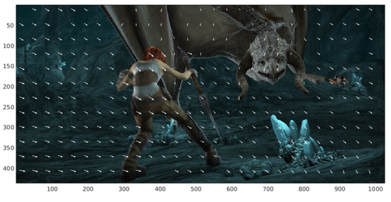
Figure 2. Correspondences of patches located uniformly in the reference image.

We compute the exhaustive matching in $N_D$ positions given by

$$N_D=\left[\frac{N_x}{D}\right]\times \left[\frac{N_y}{D}\right],$$

where $N_x$ and $N_y$ represent the height and width of the image, respectively, and [ ] represents an integer division.

3.3.2. Random Location

The random location strategy defines a grid ${\mathbf{g}}_R$ where the matching is located. In Figure 3, the matching and its correspondences are represented with white arrows. The initial point of the arrow shows the coordinates where a patch is taken in the reference images. The final part of the arrow shows the coordinates where the corresponding patch is located in the target image. In every realization of the strategy, the grid ${\mathbf{g}}_R$ is changed.

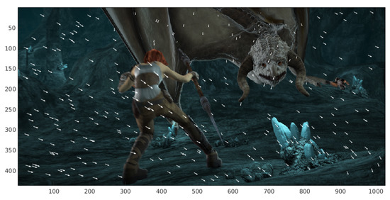
Figure 3. Correspondences of patches located randomly in the reference image.

3.3.3. Location in Maximum Values of the Gradient Magnitude

We computed the gradient magnitude of the reference image. We ordered that gradient from the smallest magnitude to the maximum magnitude. We considered the $N_D$ as the largest magnitude of the gradient. The grid ${\mathbf{g}}_g$ is defined by the $N_D$ maximum magnitude positions of the gradient in the reference image. In Figure 4, we show the correspondences given the location in the maximum magnitude of the gradient.

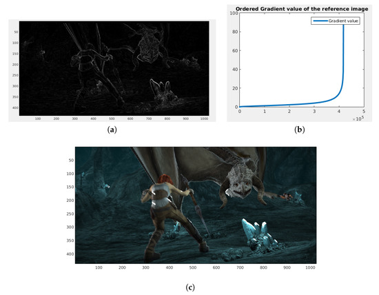
Figure 4. Correspondence of patches located in the largest magnitude of the gradient. (a) Gradient magnitude of the reference image. (b) Ordered gradient from the minimum magnitude to the maximum magnitude. (c) Correspondences of the patches located in the maximum gradient magnitudes (white arrows).

In Figure 4a, we show the computed magnitude of the gradient. We represent the magnitude of the gradient using intensities: white means the maximum magnitude of the gradient, and black means the minimum magnitude. We ordered the gradient magnitude and plotted it. We took the last $N_D$ magnitude of the gradient. These gradients correspond to locations in the image. In those locations, we performed exhaustive matching. We observe in Figure 4c that the matching is located on the edges of the girl’s cloth, on the dragon face, and on rock edges.

3.3.4. Location in the Large Magnitudes of the Gradient in a Uniform Location

The main idea is to compute matching in a location, where large gradients are present using a uniform grid (a large gradient uniform grid). We divided the gradient of the image into three subsets: a large gradient set, a medium gradient set, and a small gradient sets. In Figure 5c, we show the position of matching in the large gradient uniform grid. We show in (a) the magnitude of the gradient of the image. In (b), we show a binary image where 1 indicates the location of large gradients that coincides with regions that present edges and highly textured surfaces.

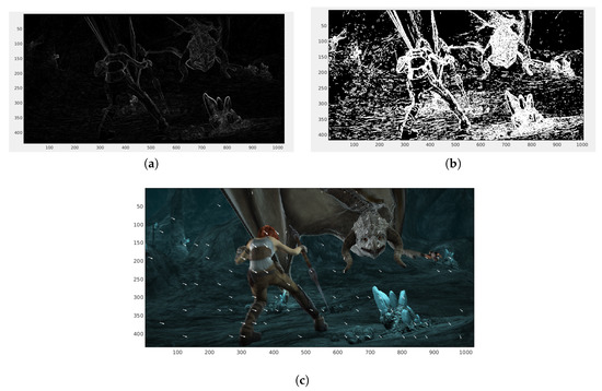
Figure 5. (a) Gradient of the reference image. (b) Large gradient set. (c) Matching result of patches located in the large gradient uniform grid.

In (c), we observe that the matching is located in a uniform location but only in places where the high gradient is present.

3.3.5. Location in the Medium Magnitudes of the Gradient in a Uniform Location

We show in Figure 6a the magnitude of the gradient of the image and the located matching In (b), we show a binary image where 1 indicates the location of medium gradients.

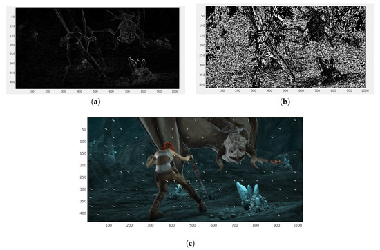
Figure 6. (a) Gradient of the reference image. (b) Medium gradient set. (c) Matching result of the patches located in the medium gradient uniform grid.

If we compare Figure 6c with Figure 5c, we observe that they are complementary; i.e., locations that are considered in one strategy are not considered in the other.

3.3.6. $\chi \left(\mathbf{x}\right)$ Value

The value of the $\chi \left(\mathbf{x}\right)$ is given by the confidence value $c\left(\mathbf{x}\right)$, i.e.,

$$\chi \left(\mathbf{x}\right)=c\left(\mathbf{x}\right).$$

(33)

The $c\left(\mathbf{x}\right)$ is the weight of matching. In the presence of auto-similarity of the target image, $c\left(\mathbf{x}\right)$ will be zero.

3.4. Pseudo Code

The model was implemented based on the available code in IPOL [1] for the TV-L1 model. The model was programmed in C in a laptop with i7 processor and 16 GB RAM. The pseudo code is presented in Algorithm 1.

The algorithm to compute the optical flow using additional information:

Algorithm 1: Integration of additional information coming from exhaustive matching

$Input$: Two consecutive color images $I_0\left(\mathbf{x}\right)$, $I_1\left(\mathbf{x}\right)$.

$Parameters$ α, λ, P, ${\theta }_0$, ${\tau }_d$, β, $MaxIter$, β, κ, $Numbe{r}_{scales}$, $Numbe{r}_{warpings}$, ${\theta }_{occ}$.

$Output$: optical flow $\mathbf{u}\left(\mathbf{x}\right)=(u_1\left(\mathbf{x}\right),u_2\left(\mathbf{x}\right))$

$\mathrm{Down-scale}{I}_0\left(\mathbf{x}\right),I_1\left(\mathbf{x}\right)$

Initialization $\mathbf{u}\left(\mathbf{x}\right)=\mathbf{v}\left(\mathbf{x}\right);w=0$

$for$ $scales\leftarrow Numbe{r}_{scales}$ to 1

Construct ψ

In specific locations defined by the strategy compute ${\mathbf{u}}_{\mathbf{e}}\left(\mathbf{x}\right)$ using Equation (31)

Using ${\mathbf{u}}_{\mathbf{e}}\left(\mathbf{x}\right)$ compute $c\left(\mathbf{x}\right)$ and update $\chi \left(\mathbf{x}\right)$.

$for$ $w\leftarrow 1$ to $Numbe{r}_{warpings}$

Compute $\alpha \left(\mathbf{x}\right)$ and occlusion $\mathbf{o}\left(\mathbf{x}\right)$.

Compute ${\mathbf{v}}_{\mathbf{i}}\left(\mathbf{x}\right)$, Equations (24) and (25).

Compute $\mathbf{u}$, Equation (21).

Compute ξ Equations (22) and (23).

update ${\kappa }_n=\kappa {\left(0.5\right)}^{scales}$

$end for$

up-sample $\mathbf{u}\left(\mathbf{x}\right)$

$end for$

Out $\mathbf{u}\left(\mathbf{x}\right)$.

4. Experiments and Database

4.1. Middlebury Database

The proposed model has been tested in the available Middlebury database training set [19]. This database contains eight image sequences, and its ground truth is also available. We divided the Middlebury sequences into two groups: (i) a training set (two sequences) and (ii) an evaluation set containing the rest of the sequences. These images present illumination changes and shadows (Figure 7e–h).

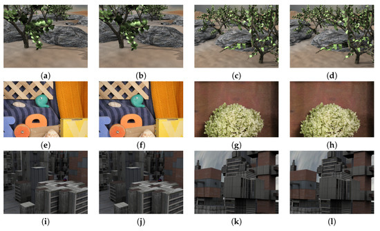
Figure 7. Images of the Middlebury database containing small displacements. (a) and (b) frame10 and frame11 of sequence Grove2, respectively. (c) and (d) frame10 and frame11 of sequence Grove3, respectively. (e) and (f) frame10 and frame11 of sequence RubberWhale, respectively. (g) and (h) frame10 and frame11 of sequence Hydrangea, respectively. (i) and (j) frame10 and frame11 of sequence Urban2, respectively and finally (k) and (l) of sequence Urban2, respectively.

Figure 7 shows two consecutive frames, namely, Frame 10 and Frame 11. In our model, $I_0$ corresponds to Frame 10, $I_1$ to Frame 11. Figure 7a,b correspond to the Grove2 sequence, (c) and (d) to he Grove3 sequence, (e) and (f) to RubberWhale, (g) and (h) to the Hydra sequence, (i) and (j) to the Urban2 sequence, and (k) and (l) to the Urban3 sequence.

4.2. The MPI-Sintel Database

The MPI-Sintel database [20] presents long synthetic video sequences containing large displacements and several image degradations as blur or reflections as well as different effects such as fog, shadows, reflections, and blur.

Moreover, there are two versions of the MPI-Sintel database: clean and final. The final version is claimed to be more challenging and includes all effects previously mentioned. For our evaluation, we take the final version of MPI-Sintel. In Figure 8 we compare the same frame extracted from clean version and final version.

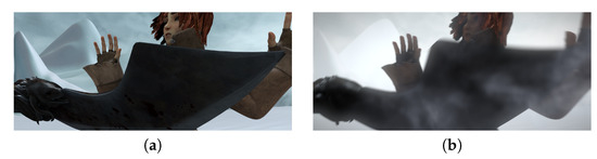
Figure 8. Image extracted from MPI-Sintel clean version and MPI-Sintel final version. We extracted frame_0014 from sequence ambush_2. (a) frame_0014 clean version. (b) frame_0014 final version.

In Figure 8a we show the clean version of frame_0014 of sequence ambush_2. The Figure 8b includes fog and blur effects making this MPI-Stintel version more challenging.

The optical flow (ground truth) of this database is publicly available in order to compare different algorithms. The optical flow was color-coded using the color code presented in Figure 9.

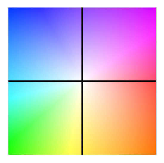
Figure 9. Color code used for the optical flow.

Figure 10 displays some examples of the MPI-Sintel database. There are images with large displacements: around 170 pixels for the cave_4 sequence and around 300 pixels for temple_3. In the cave_4 sequence, a girl fights with a dragon inside a cave, shown in Figure 10a,b,d,e. In (a) and (b), the girl moves her lance to attack the dragon. In (d) and (e), the dragon moves its jaws very fast. In (g) and (h), we show the girl trying to catch the small dragon, but a claw appears and takes the small dragon away. In (j) and (k), the girl falls in the snow. We observe large displacement and deformation with respect to her hands. We also display the optical flow of the video sequence.

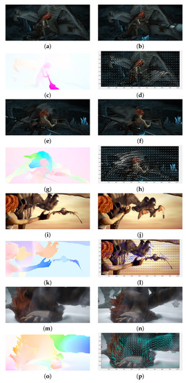
Figure 10. Examples of images of the MPI-Sintel database video sequence. (a,b) frame_0010 and frame_0011, (c) color-coded ground truth optical flow of the cave_4 sequence, (d) ground truth represented with arrows. (e,f) frame_0045 and frame_0046, (g) color-coded ground truth, and (h) arrow representation of optical flow of the cave_4 sequence, (i,j) frame_0030 and frame_0031, (k) color-coded ground truth optical flow, (l) arrow representation (in blue) of the temple3 sequence. (m,n) frame_0006 and frame_0007, (o) color-coded ground truth and (p) arrow representation (in green) ground truth optical flow of the ambush_4 sequence.

We present in Table 1 the number of images and the names of each sequence of the final MPI-Sintel.

Table 1. Number of images in each image sequence.

Sequence Name	Number of Images
alley	100
ambush	174
bamboo	100
bandage	100
cave	100
market	140
mountain	50
shaman	100
sleeping	100
temple	100
Total images	1064

4.3. Experiments with the Middlebury Database

In this section, we present quantitative results obtained by the optical flow estimation model presented above. We have divided the database in the training set and the evaluation set. We used the sequences Grove3 and RubberWhale as the training set (TRAINING_SET). The other sequences are used to validate the method.

4.4. Parameter Estimation

Initially, we estimated the best parameters in our training set considering $\kappa =0.0$, i.e., the model cannot handle large displacements. We scan the parameter θ and λ, setting $\tau =1.0$ and $\beta =0.0$ and estimating the $EPE$ (End Point Error) and $AAE$ (Average Angular Error) error.

We obtained the minimum value for both $EPE$ and $AAE$ error in $\theta =0.1$ and $\lambda =0.1$. We selected these parameter values. In Figure 11, we show the obtained optical flow, setting θ and λ parameters.

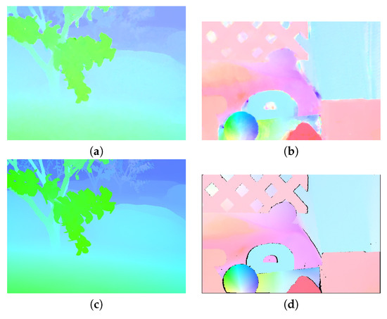
Figure 11. Color-coded optical flow. (a) Color-coded optical flow for Grove2. (b) Color-coded optical flow for RubberWhale. (c) Ground truth for the Grove2 sequence. (d) Ground truth for the RubberWhale sequence.

With these parameters we obtained an average $EPE=0.16$ and $AAE=3.78$.

We fixed the value of θ and λ and then varied ${\tau }_d$ from $0.1$ to $2.3$ and β from 1 to 8. We obtained a minimum in ${\tau }_d=1.9$ and $\beta =2.0$. With these parameters we obtained and average $EPE=0.1369$ and $AAE=3.1186$. In Figure 11c,d, we present the ground truth for the Grove2 sequence and the RubberWhale sequence, respectively, in order to facilitate the visual evaluation of our results.

In Figure 12, we show the optical flow and the weight map $\alpha \left(\mathbf{x}\right)$.

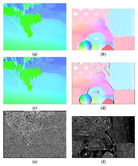
Figure 12. Color-coded optical flow. (a) Color-coded coded optical flow for Grove2. (b) Color-coded optical flow for RubberWhale. (c) Ground truth for the Grove2 sequence. (d) Ground truth for the RubberWhale sequence. (e) Weight map $\alpha \left(\mathbf{x}\right)$ for Grove2. (f) Weight map $\alpha \left(\mathbf{x}\right)$ for RubberWhale.

We can observe in Figure 12a,b the obtained optical flow using weight map $\alpha \left(\mathbf{x}\right)$. There is an improvement in both estimated optical flows. In (c) and (d), we present the $\alpha \left(\mathbf{x}\right)$ function for both sequences. Low gray levels represent low values of $\alpha \left(\mathbf{x}\right)$; i.e., the model uses the gradient constancy assumption. Higher gray level means that the model uses the brightness constancy assumption. As we can see in (d), the model uses gradients on shadows in the right side of the whale and the left side of the wheel. In (c), in most locations, $\alpha \left(\mathbf{x}\right)=0.5$.

4.5. Experiments with MPI-Sintel

We performed two evaluations: $\mathbf{A}$ and $\mathbf{B}$. Evaluation $\mathbf{A}$ considers the proposed model, evaluating different strategies to locate matching. These strategies are (i) uniform locations, (ii) random locations, (iii) locations in maximum gradients of the reference image, (iv) uniform locations in the largest gradients of the image, and (v) uniform locations in the medium gradients of the reference image. In these five evaluations, the matching was computed comparing colors between pixels. Additionally, we performed the previous five evaluations using gradient patches instead of color patches.

In Evaluation $\mathbf{B}$, considering the extended Horn-Schunck model, we evaluated its performance in different location strategies. These strategies are the same in Evaluation $\mathbf{A}$, i.e., (i) uniform, (ii) random, (iii) maximum gradients, (iv) uniform locations in maximum gradients, and (v) uniform locations in medium gradients.

4.6. Parameter Estimation of the Proposed Model with MPI-Sintel

4.6.1. Parameter Model Estimation

Parameters λ, θ, and β y ${\tau }_b$ were estimated by the PSO algorithm [21]. The PSO algorithm is an optimization method that does not compute derivatives of the functional to minimize. It minimizes a functional by iteratively trying to improve many candidate solutions. Each iteration is performed taking into account the functional, and it is minimized considering these candidate solutions and updating them in the space-domain according to dynamics behavior for the position and velocity of solution candidates. Let $f:{\mathbb{R}}^n:\to \mathbb{R}$ be a functional to optimize (in this case, we considered the total $EPE$ as the functional to minimize), where n is the number of parameters to estimate. Let ${\mu }_i$ be a candidate solution that minimizes the optical flow estimation error. In each iteration, a global best candidate parameter is stored (${\mu }_g$) and jointly is stored the parameter candidate that presents the best performance in the iteration (${\mu }_b$). Each parameter vector ${\mu }_i$ is updated by

$${\nu }_i^{t+1}=\omega {\nu }_i^t+{\phi }_g({\mu }_i^t-{\mu }_g)+{\phi }_b({\mu }_i^t-{\mu }_b)$$

$${\mu }_i^{t+1}={\mu }_i^t+{\nu }_i^t$$

where ω is the evolution parameter for each solution ${\mu }_i$, and ${\phi }_g$ and ${\phi }_b$ are positive weight parameters. A saturation for ${\nu }_i$ is usually considered. In our case, we used ${\nu }_{max}=2$ and ${\nu }_{min}=-2$. In Table 2, we show the parameters of our PSO algorithm.

Table 2. PSO parameters.

Parameter	Value
NIndividuals	3
NGeneration	20
NSequences	8
$\omega$	0.5
${\phi }_g$	0.5
${\phi }_b$	1.0

In each estimated optical flow of the sequence, we computed the $EPE$ and $AAE$ for each sequence, and each PSO iteration we minimized the following functional:

$$J(\lambda ,\theta ,\beta ,{\tau }_d)=\sum _{i=1}^8\left(EP{E}_i+AA{E}_i\right)$$

(34)

where $EP{E}_i$ and $AA{E}_i$ is the end point error and the average angular error of each considered sequence, respectively, defined as

$$\begin{array}{c}\hfill {\displaystyle cEPE=\frac{1}{n}\sum _{i=1}^n\sqrt{{(g_{1i}-u_{1i})}^2+{(g_{2i}-u_{2i})}^2}}\\ \hfill {\displaystyle AAE=\frac{1}{n}\sum _{i=1}^{n}co{s}^{-1}\left(\frac{1+g_{1i}{u}_{1i}+g_{2i}{u}_{2i}}{\sqrt{1+g_{1i}^2+g_{2i}^2}\sqrt{1+u_{1i}^2+u_{2i}^2}}\right)}\end{array}$$

(35)

where $\mathbf{g}\left(\mathbf{x}\right)=(g_1\left(\mathbf{x}\right),g_2\left(\mathbf{x}\right))$ is the ground truth optical flow, and $\mathbf{u}\left(\mathbf{x}\right)=(u_1\left(\mathbf{x}\right),u_2\left(\mathbf{x}\right))$ is the estimated optical flow.

In order to estimate the parameters of the model, we selected eight pairs of consecutive images video sequences of the MPI-Sintel database. We selected the first two images from sequences: alley_1, ambush_2, bamboo_2, cave_4, market_5, bandage_1, mountain_1, and temple_3.

In Figure 13, we show image sequences used to estimate the parameter, the ground truth optical flow, and our results.

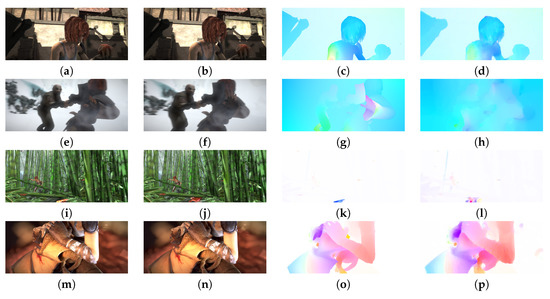
Figure 13. Image sequences used to estimate model parameters. In the parameter estimation, we used the first two frames of each considered sequence: (a–d) the frames of the alley_1 sequence, the ground truth, and our results, respectively. (e,f) the ambush_2 sequence, (g) the ground truth, and (h) our result. (i,j) frames of the bamboo_2 sequence, (k) the ground truth, and (l) our result. (m,n) the frame of bandage_1 sequence (o) the ground truth, and (p) our results.

We observe in Figure 13a,b a girl that moves a fruit upward. Our method estimates correctly the direction of the motion. $EPE=0.22$. Figure 13e,f show the lance as well as the girl and the man fighting. The method cannot estimate correctly the motion due to large displacements. $EPE=10.21$. Figure 13l shows that the large displacements of the butterfly cannot be correctly estimated. In Figure 13p, we observe that the displacements are correctly estimated. $EPE=0.78$.

In Figure 14b, we show the performance of the PSO algorithm minimizing the functional in Equation (34).

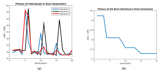
Figure 14. Performance of the PSO algorithm. (a) Performance of each individual. (b) Performance of the best individual in each generation.

Figure 14a shows the performance of each individual for 20 generations. It is observed that the variation of the performance decreases along the iterations. In Figure 14, the performance of the best individual for each iteration decreases its functional value; the final value is $17.29$.

We present in Table 3 the final $EPE$ and $AAE$ value for our selected training set.

Table 3. Results obtained by PSO in the MPI-Sintel selected training set.

	alley_1	ambush_4	bamboo_2	bandage_1	cave_4	market_5	mountain_1	temple_3
$EPE$	$0.22$	$10.21$	$0.23$	$0.78$	$3.49$	$18.37$	$9.71$	$6.50$
$AAE$	$2.30$	$6.68$	$4.32$	$7.25$	$11.91$	$25.53$	$0.74$	$30.07$

As is shown in Table 3, the best performance was for the sequence alley_1 that presents small displacements, and the worst performance was for the sequence market_5, which presents large displacements. Final parameters for the proposed model are $\lambda =0.2894$, $\theta =0.1422$, $\beta =1.2303$, and ${\tau }_d=0.5687$.

4.6.2. Exhaustive Search Parameter Estimation

Parameters P and D are estimated once the model parameter is estimated. Because these parameters are discrete, we estimate them, scanning P and D values in an exhaustive way. We varied P from 2 to 20 pixels with a step of 2 pixels, and D varied from 32 to 64 with a step of 4 pixels. In Figure 15, we show the obtained performance by the functional in Section 4.6.1 for the MPI-Sintel selected video sequences.

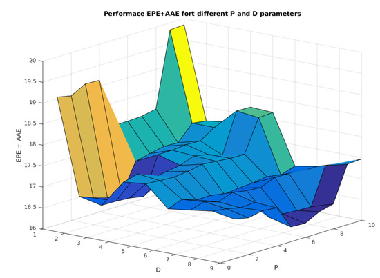
Figure 15. Performance of the proposed model considering variation in P and D parameters.

We show in Figure 15 the performance $EPE+AAE$ for a different grid size D and for a different patch size P. It is observed that the minimum of the surface is located at $D=64$ and $P=12$, reaching a performance of $16.33$. We prefer the second minimum located at $D=36$ and $P=8$, reaching a performance of $16.53$. This second minimum implies a more dense grid that would perform better in terms of handling small objects. The model using patches outperforms the original model, which does not consider exhaustive search correspondences.

4.7. Parameter Estimation of the Extended Horn-Schunk

4.7.1. ${\alpha }_{hs}$ Parameter

The multi-scale model has a principal parameter α. This parameter represents the balance between the data term and regularization. We adjusted this parameter using the selected training set which contains eight video sequences. In Figure 16, we show the obtained $EPE+AAE$ values for different α values:

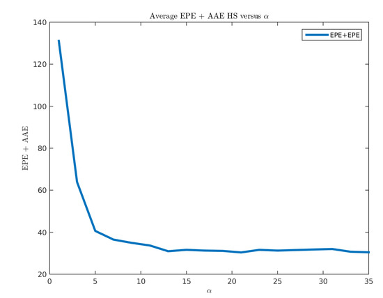
Figure 16. Performance of the Horn-Schunck method for different ${\alpha }_{hs}$ values.

Figure 16 shows that the minimum value of the error is reached for ${\alpha }_{hs}=32$. We presented in Table 4 the performance obtained by Horn-Schunck for each sequence.

Table 4. Results obtained by PSO in the MPI-Sintel selected training set.

	alley_1	ambush_4	bamboo_2	bandage_1	cave_4	market_5	mountain_1	temple_3
$EPE$	$0.48$	$16.72$	$0.34$	$1.81$	$5.47$	$24.82$	$1.14$	$9.47$
$AAE$	$4.81$	$10.79$	$6.27$	$26.57$	$22.69$	$37.87$	$14.96$	$61.54$

Total average $EPE$ and $AAE$ is $7.53$ and $23.19$, respectively. If we compare this with Table 3, where the results of our proposed model are presented, it is evident that the proposed model outperforms the extended Horn-Schunck model.

4.7.2. Exhaustive Search Parameter Estimation

We varied the P and D with discrete steps in order to find the combination to improve the performance of the optical flow estimation. The parameter P varied from 2 to 20 with a step of 2 pixels, and D varied from 32 to 64 with a step of four pixels. We evaluated the performance of the extended Horn-Schunck method in the selected training set. In Figure 17, we present the obtained results of this experiment.

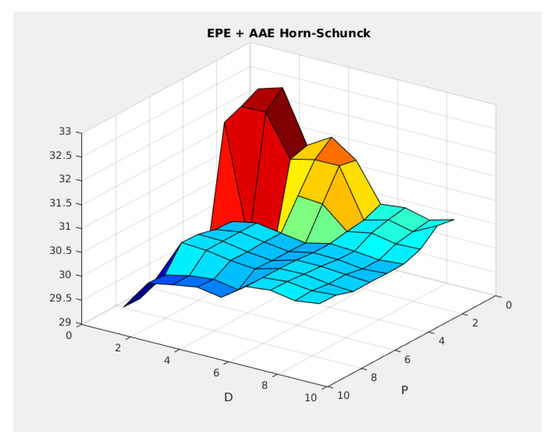
Figure 17. Performance of the Horn-Schunck model for different P and D parameters.

For these parameters, the obtained $EPE$ and $AAE$ are presented in Table 5.

Table 5. Results obtained by the PSO in the MPI-Sintel selected training set.

	alley_1	ambush_4	bamboo_2	bandage_1	cave_4	market_5	mountain_1	temple_3
$EPE$	$0.48$	$16.87$	$0.34$	$1.80$	$6.42$	$23.30$	$1.15$	$8.92$
$AAE$	$4.77$	$10.89$	$6.22$	$26.32$	$22.94$	$34.87$	$14.97$	$55.27$

Comparing this table with Table 4, we observe that in sequence alley_1, bandage_1, market_5, and temple_3, there is an improvement in performance. Sequences ambush_2, bamboo_2, and mountain_1 approximately maintain the performance. Sequence cave_4 present an increment in the $EPE$ from $5.47$ to $6.42$. On average, the total performance is $EPE=7.41$ and $AAE=22.11$, which represent an improvement compared with the results obtained in Table 4.

5. Results

5.1. Reported Results in Middlebury

We show in Table 6 the reported values for TV-L1 in [1] using gray level images of the Middlebury database.

Table 6. The reported performance of TV-L1 in Middlebury [1].

Error	Dime	Grove3	Hydra	Urban3	Venus	Average
$EPE$	0.162	0.721	0.258	0.711	0.394	0.4492
$AAE$	2.888	6.590	2.814	6.631	6.831	5.1508

In Table 7, we present our results obtained using the set of parameters determined above.

Table 7. Obtained results of our model in Middlebury with $\kappa =0.0$.

Error	Dime	Grove3	Hydra	Urban3	Venus	Average
$EPE$	0.0925	0.7090	0.1729	0.7078	0.3492	0.4063
$AAE$	1.8248	6.5913	2.0626	6.9080	6.0818	4.6937

In Table 7, we observe that, in most cases, the obtained result is similar to that reported in [1]. For real sequences Dime and Hydra, our model outperforms the model in [1]. In the sequence Urban3, our method presents a larger error ($AAE$) than that given in Table 6.

5.2. Specific Location of Matching $\kappa \ne 0$

Considering the integration of exhaustive matching to our variational model, we perform an empirical evaluation to determine the best location of exhaustive matching in order to improve the optical flow estimation. We compare three strategies to locate exhaustive matching: (i) uniform location in a grid ${\mathcal{G}}_{\mathcal{D}}\subset \mathrm{\Omega }$, (ii) random location of matching, and (iii) matching located in the maximum of the magnitude of the gradient.

5.2.1. Uniform Locations

This is the most simple strategy to locate exhaustive matching. Location depends on the size of the grid ${\mathcal{G}}_{\mathcal{D}}$.

In Figure 18, we present exhaustive correspondences computed in a uniform grid. We present a zoomed area for Grove2 and Rubberwhale sequences.

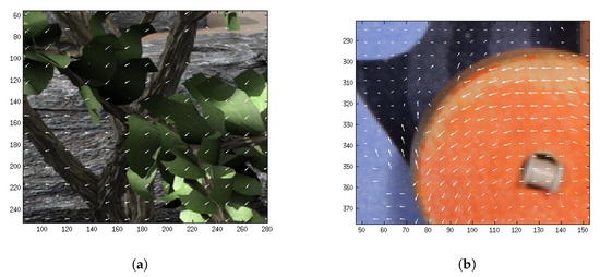
Figure 18. Exhaustive matching represented with white arrows. (a) Exhaustive matching using $D=18$ and $P=10$ for Grove2. (b) Exhaustive matching using $D=6$ and $P=8$ for Rubberwhale.

We vary these parameters P and D from 2 to 10 and from 2 to 18, respectively. The minimum of the error is obtained for large values of D since the exhaustive search frequently yields some false matching, as can be seen in Figure 18b. Increasing the D parameter produces more confident matching. Thus, we select $P=4$ and $D=16$. With these parameters, we include in the model around 900 matches. Considering these selected parameters, we obtained an average of $EPE=0.1332$ and $AAE=3.0080$ in TRAINING_SET. In VALIDATION_SET, we obtained the results showed in Table 8.

Table 8. Results obtained by the uniform matching location strategy in VALIDATION_SET.

Error	Dime	Grove3	Hydra	Urban3	Venus	Average
$EPE$	0.0975	0.6924	0.1672	0.4811	0.3034	0.3485
$AAE$	1.8739	6.4759	2.0160	4.334	4.2259	3.7872

For the Urban3 sequence, we used $P=24$ and $\alpha \left(\mathbf{x}\right)=1.0$. This image is produce by CGI and presents auto-similarities.

5.2.2. Random Locations

We performed experiments locating the matching and using a grid created randomly. We computed around 900 matches in each experiment. We performed each experiment three times, obtaining results shown in Table 9.

Table 9. Average $EPE$ and $AAE$ obtained by Random Location Strategy in VALIDATION_SET set.

Error	Dime	Grove3	Hydra	Urban3	Venus	Average
$EPE$	0.0967	0.6798	0.1666	0.5446	0.2988	0.3573
$AAE$	1.8876	6.3781	2.0214	4.8060	4.1977	3.8581

5.2.3. Locations for Maximum Magnitudes of the Gradient

We present in Table 10 our results using the maximum gradient.

Table 10. Average $EPE$ and $AAE$ obtained by the maximum gradient location strategy in VALIDATION_SET.

Error	Dime	Grove3	Hydra	Urban3	Venus	Average
$EPE$	0.0938	0.7147	0.1772	0.7338	0.3014	0.4042
$AAE$	1.8596	6.5793	2.1159	5.9172	4.3285	4.1601

Comparing the average $EPE$ and $AAE$ obtained for each strategy, we observe that the best performance was obtained by the uniform location strategy, the second best performance by the random location strategy, the third best by the maximum gradient strategy.

5.3. Evaluation in MPI-Sintel

5.3.1. Uniform Location

As a first experiment, we computed the optical flow for the whole MPI-Sintel training database. We did not compute the optical flow in the images used to estimate the parameters of the algorithm. We computed 1033 optical flow and evaluated its $EPE$ and $AAE$ for each sequence. In Table 11, we present our results for MPI-Sintel:

Table 11. Summary of results. The end point error and average angular error obtained by uniform locations in the MPI-Sintel training set.

Sequence Name	$\mathit{EPE}$	$\mathit{AAE}$
alley	0.36	3.05
ambush	19.72	26.07
bamboo	1.68	13.66
bandage	0.64	7.01
cave	9.26	13.13
market	8.79	13.61
mountain	1.02	10.29
shaman	0.38	7.18
sleeping	0.11	1.79
temple	9.94	13.71
Total $EPE$	5.58	10.87
$EPE+AAE$	16.45

In Table 11, we show our obtained results by our proposed model using uniform location. We obtained $5.58$ as the $EPE$ error. We observe that the best performance was obtained for the sleeping sequence. This sequence presents the dragon and the sleeping girl and contains small displacements. The worst performance was obtained for the Ambush sequence, where the girl fights with a man in the snow. This sequence presents extremely large displacements that are very hard to handle.

5.3.2. Random Location

In the second experiment, we computed the optical flow for the MPI-Sintel training set. We performed two realizations of the optical flow estimation and computed the $EPE$ and $AAE$ average value on these realizations. In Table 12, we present our results:

Table 12. Summary of results. The end point error and average angular error obtained by random locations in the MPI-Sintel training set.

Sequence Name	$\mathit{EPE}$	$\mathit{AAE}$
alley	0.36	3.04
ambush	19.59	25.70
bamboo	1.69	13.69
bandage	0.64	7.02
cave	9.54	13.52
market	8.78	13.72
mountain	1.02	10.31
shaman	0.38	7.19
sleeping	0.11	1.79
temple	10.16	14.03
Total $EPE$	5.62	10.91
$EPE+AAE$	16.53

5.3.3. Location on Maximum Gradients

In the third experiment, we computed the optical flow for the MPI-Sintel training set. We performed matching with patches located in the maximum gradient magnitude of the current frame. Our obtained results are presented in Table 13.

Table 13. Summary of results. The end point error and average angular error obtained by locations on maximum gradients in the MPI-Sintel training set.

Sequence Name	$\mathit{EPE}$	$\mathit{AAE}$
alley	0.37	3.05
ambush	19.83	26.50
bamboo	1.66	13.56
bandage	0.65	7.04
cave	9.72	14.18
market	8.88	13.78
mountain	1.00	10.22
shaman	0.37	7.12
sleeping	0.11	1.79
temple	9.90	14.46
Total $EPE$	5.64	11.10
$EPE+AAE$	16.73

5.4. Summary

We summarize our results of these three sections in Table 14.

Table 14. Summary of the obtained results for different strategies.

Strategy	$\mathit{EPE}$	$\mathit{AAE}$
Uniform	5.58	10.87
Random	5.62	10.91
Maximum Gradient	5.64	11.10

The best performance of these three strategies was obtained by uniform locations. We processed the MIP-Sintel test database and uploaded our results to the website http://www.sintel.is.tue.mpg.de/results. The test database consists of eight sequences of 500 images in two versions: clean and final. The final MPI-Sintel version considers effects such as blur, shadows, illumination changes, and large displacements. This database is very challenging and represents the state-of-the-art evaluation dataset.

In Figure 19, we show the position reached by our method:

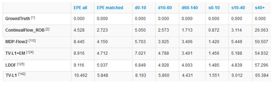
Figure 19. Obtained results by our method in the MPI-Sintel test database (at 18 October 2018).

In Figure 19, we can observe that our method (TV-L1+EM) obtained $EPE=8.916$ and is located in Position 124 of the 155 methods. Our proposal outperforms TV-L1 and LDOF. Our performance is similar to that obtained by MDP-Flow2 [3].

5.4.1. Combined Uniform–Large Gradient Locations

We obtained the best performance using uniform locations, so we decided to mix two strategies: uniform locations with large gradient locations. In order to implement this new strategy, we took the magnitude of the gradient of the reference frame and ordered them from large to small values. We then considered the first third of this ordered data as a large gradient and the second third of the data as the medium gradient. Pixels in the reference frame can belong to a large gradient set, a medium gradient set, or a small gradient set. In uniform locations where the gradient of pixels belongs to the large gradient, we set $\chi \left(x\right)=1$; else, we set $\chi \left(x\right)=0$.

In Table 15, we show our results obtained by this strategy using the MPI-Sintel database.

Table 15. Summary of results. The end point error and average angular error obtained by the combination of uniform and large gradients in the MPI-Sintel training set.

Sequence Name	$\mathit{EPE}$	$\mathit{AAE}$
alley	0.36	3.03
ambush	19.85	26.43
bamboo	1.70	13.60
bandage	0.65	7.03
cave	9.84	14.39
market	9.10	14.07
mountain	0.98	10.24
shaman	0.38	7.16
sleeping	0.11	1.78
temple	10.03	14.31
Total $EPE$	5.70	11.14
$EPE+AAE$	16.83

We observe in Table 15 that the performance of the strategy is outperformed by the uniform locations strategy. It seems that those two conditions, uniform location and large gradients, eliminate good correspondences located in medium or small gradients magnitude.

5.4.2. Combined Uniform–Medium Gradient Locations

We combined the location between uniform and medium gradient locations.

In Table 16, we show our results obtained by this combined strategy in the MPI-Sintel database.

Table 16. Summary of results. The end point error and average angular error obtained by the combination of uniform and medium gradients in the MPI-Sintel training set.

Sequence Name	$\mathit{EPE}$	$\mathit{AAE}$
alley	0.63	5.99
ambush	26.42	34.81
bamboo	3.16	27.47
bandage	1.19	18.21
cave	12.49	19.18
market	10.76	19.90
mountain	1.43	13.57
shaman	0.67	14.39
sleeping	0.14	2.44
temple	16.21	26.23
Total $EPE$	5.67	11.10
$EPE+AAE$	16.77

We observe in Table 16 that the performance of the strategy is outperformed by the uniform locations strategy. It seems that those two conditions, uniform location, and medium gradients, eliminate good correspondences located in large or small gradients magnitude.

5.4.3. Results Obtained by Horn-Schunck

As a starting point, we evaluated the implementation of Horn-Schunck in [18] in MPI-Sintel. The obtained results are shown in Table 17.

Table 17. Summary of results. The end point error and average angular error obtained by Horn-Schunck in the MPI-Sintel training set.

Sequence Name	$\mathit{EPE}$	$\mathit{AAE}$
alley	0.36	3.02
ambush	19.91	26.46
bamboo	1.67	13.59
bandage	0.65	7.03
cave	9.77	14.32
market	9.10	14.07
mountain	0.99	10.24
shaman	0.38	7.16
sleeping	0.11	1.79
temple	9.80	13.90
Total $EPE$	7.76	17.74
$EPE+AAE$	25.50

In Table 17, we show the performance obtained by the Horn-Schunck method using $\alpha =32$. The performance $EPE+AAE=25.50$ is almost double the performance of our proposed model.

5.4.4. Results Obtained by Horn-Schunck Using Uniform Locations

We performed the evaluation of MPI-Sintel using the extended version of Horn-Schunck to handle large displacements. In Table 18, we show the obtained results:

Table 18. Summary of results. The end point error and average angular error obtained by Horn-Schunck using uniform locations in the MPI-Sintel training set.

Sequence Name	$\mathit{EPE}$	$\mathit{AAE}$
alley	0.64	6.07
ambush	26.01	34.88
bamboo	3.52	28.04
bandage	1.19	18.14
cave	34.44	45.41
market	11.74	20.60
mountain	1.59	14.33
shaman	0.66	11.85
sleeping	0.29	2.95
temple	17.33	27.95
Total $EPE$	10.16	20.95
$EPE+AAE$	30.76

In Table 18, we show that the performance obtained by the Horn-Schunck using patches in uniform locations is outperformed by the results in Table 17. This extended version of Horn-Schunck presents $EPE+AAE=30.76$. We explain this fact considering correct and false correspondences (outliers) given by the exhaustive search. The Horn-Schunck model is not robust to outliers because the method considers in its formulation an $L^2$ data term and an $L^2$ regularization term. On the other hand, $TV-L1$ is robust to outliers and performs better using additional information.

6. Discussion

We present here a method to estimate optical flow for realistic scenarios using two consecutive color images. In realistic scenarios, occlusions, illumination changes, and large displacements occur. Classical optical flow models may fail in realistic scenarios. The presented model incorporates the occlusion information on its energy based on the maximum error of the optical flow estimation.

This model handles illumination changes using a balance-term between gradients and intensities. The inclusion of this balance term allows the model to improve the performance of the optical flow estimation in scenarios with illumination changes, reflections, and shadows.

Thanks to the use of supplementary matching (given by exhaustive searches in specific locations), this model is able to handle large displacements.

We tested five strategies of specific matching locations: uniform locations, random locations, maximum gradient locations, uniform-maximum gradient locations, and uniform-medium gradient locations. The obtained results show that the best performance was obtained by the uniform location strategy and the second best performance was achieved by the random location strategy. Empirically, we demonstrated that the best criteria to localize exhaustive matching does not depend on image gradients but on a uniform spatial location. Additionally, we have used gradient patches instead of color patches to compute correspondences and have used this information in order to estimate optical flow. The obtained results show that the use of gradient patches outperform the model based on color.

We also tested the classical Horn-Schunk model and extended it to handle additional information coming from an exhaustive search. The obtained results show that this extended Horn-Schunck model cannot handle large displacements in this way due to the presence of many outliers given by the exhaustive search. The Horn-Schunck model uses an $L^2$ norm in its formulation, which is not robust to outliers. On the other hand, the proposed model that uses the $TV-L1$ norm is robust to outliers and performs better using additional information. The use of an occlusion estimation that depends on optical flow error lets us eliminate simultaneously false exhaustive correspondences and good correspondences. Some correspondences (i.e., good correspondences) present large errors due to illumination changes, blur, reflections, shadows, or fog that may be present in the MPI-Sintel sequence. These correspondences are eliminated because they present large optical flow errors.

We estimated parameters of the model using the PSO algorithm, which helped us to improve the global performance based on the $EPE$ and $AAE$ error computed in a training subset of MPI-Sintel. The final result obtained in the whole database was similar to the one obtained in this small dataset. That means that the small dataset was representative of the database.

The proposed model needs a methodology to validate matching processes. This new methodology should assign to each match a reliable value in order to eliminate false matching.

The number of good matching is necessary to be increased in order to improve optical flow estimations. One way to do that is by the use of deformable patches. Performing an exhaustive search using deformable patches is necessary to have a good correspondence between two patches of the reference frame and the target frame. Once a good correspondence in the target frame is found, a patch in the reference frame can be divided into smaller patches. For each smaller patch, a local search on the target image can be performed in order to increase the number of matching.

References

- Sánchez, J.; Meinhardt-Llopis, E.; Facciolo, G. TV-L1 Optical Flow Estimation. Image Process. Line 2013, 2013, 137–150. [Google Scholar] [CrossRef]
- Horn, B.K.P.; Schunck, B.G. Determining Optical Flow. Artif. Intell. 1981, 17, 185–204. [Google Scholar] [CrossRef]
- Xu, L.; Jia, J.; Matsushita, Y. Motion Detail Preserving Optical Flow. In Proceedings of the IEEE CVPR, San Francisco, CA, USA, 13–18 June 2010. [Google Scholar]
- Palomares, R.P.; Haro, G.; Ballester, C. A Rotation-Invariant Regularization Term for Optical Flow Related Problems. In Lectures Notes in Computer Science, Proceedings of the ACCV’14, Singapore, 1–5 November 2014; Springer: Cham, Switzerland, 2014; Volume 9007, pp. 304–319. [Google Scholar]
- Wedel, A.; Pock, T.; Zach, C.; Bischof, H.; Cremers, D. An Improved Algorithm for TV-L1 Optical Flow, Statistical and Geometrical Approaches to Visual Motion Analysis. In Proceedings of the International Dagstuhl Seminar, Dagstuhl Castle, Germany, 13–18 July 2008; Volume 5604. [Google Scholar]
- Brox, T.; Bregler, C.; Malik, J. Large Displacemnet Optical Flow. In Proceedings of the IEEE Conference on Computer Vision and Pattern Recognition, Miami Beach, FL, USA, 20–25 June 2009. [Google Scholar]
- Stoll, M.; Volz, S.; Bruhn, A. Adaptive Integration of Features Matches into Variational Optical Flow Methods. In Proceedings of the 11th Asian Conference on Computer Vision, Daejeon, Korea, 5–9 November 2012. [Google Scholar]
- Lazcano, V. Some Problems in Depth Enhanced Video Processing. Ph.D. Thesis, Universitat Pompeu Fabra, Barcelona, Spain, 2016. Available online: http://www.tdx.cat/handle/10803/373917 (accessed on 17 October 2018).
- Bruhn, A.; Weickert, J.; Feddern, C.; Kohlberger, T.; Schnoerr, C. Real-time Optical Flow Computation with Variational Methods. In Proceedings of the International Conference on Computer Analysis of Images and Patterns, Groningen, The Netherlands, 25–27 August 2003; pp. 222–229. [Google Scholar]
- Weinzaepfel, P.; Revaud, J.; Harchaoui, Z.; Schmid, C. DeepFlow: Large displacement optical flow with deep matching. In Proceedings of the IEEE International Conference on Computer Vision, Sydney, Australia, 1–8 December 2013. [Google Scholar]
- Timofte, R.; van Gool, L. Sparseflow: Sparse matching for small to large displacement optical flow. In Proceedings of the 2015 IEEE Winter Conference on Applications of Computer Vision, Waikoloa, HI, USA, 5–9 January 2015. [Google Scholar]
- Kennedy, R.; Taylor, C.J. Optical flow with geometric occlusion estimation and fusion of multiple frames. In Energy Minimization Methods in Computer Vision and Pattern Recognition, Proceedings of the International Workshop on Energy Minimization Methods in Computer Vision and Pattern Recognition, Hong Kong, China, 13–16 January 2015; Springer: Cham, Switzerland, 2015; Volume 8932, pp. 364–377. [Google Scholar]
- Fortun, D.; Bouthemy, P.; Kervrann, C. Aggregation of local parametric candidates with exemplar-based occlusion handling for optical flow. Comput. Vis. Image Underst. 2016, 145, 81–94. [Google Scholar] [CrossRef]
- Lazcano, V.; Garrido, L.; Ballester, C. Jointly Optical Flow and Occlusion Estimation for Images with Large Displacements. In Proceedings of the 13th International Joint Conference on Computer Vision, Imaging and Computer Graphics Theory and Applications, Madeira, Portugal, 27–29 January 2018; Volume 5, pp. 588–595. [Google Scholar] [CrossRef]
- Lazcano, V. Study of Specific Location of Exhaustive Matching in Order to Improve the Optical Flow Estimation. Information Technology—New Generations. In Proceedings of the 15th International Conference on Information Technology, Las Vegas, NV, USA, 16–18 April 2018; pp. 603–661. [Google Scholar]
- Steinbruecker, F.; Pock, T.; Cremers, D. Large Displacement Optical Flow Computation without Warping. In Proceedings of the 2009 IEEE 12th International Conference on Computer Vision, Kyoto, Japan, 29 September–2 October 2009; pp. 185–203. [Google Scholar]
- Xiao, J.; Cheng, H.; Sawhney, H.; Rao, C.; Isnardi, M. Bilateral Filetring-based Flow Estimation with Occlusion Detection. In Proceedings of the European Conference on Computer Vision, Graz, Austria, 7–13 May 2006; pp. 221–224. [Google Scholar]
- Meinhardt-Llopis, E.; Sanchez, J.; Kondermann, D. Horn-Schunck Optical Flow with a Multi-Scale Strategy. Image Processing Line 2013, 2013, 151–172. [Google Scholar] [CrossRef]
- Baker, S.; Scharstein, D.; Lewis, J.; Roth, S.; Black, M.; Szelinsky, R. A Database and Evaluation Methodology for Optical Flow. Int. J. Comput. Vis. 2011, 92, 1–31. [Google Scholar] [CrossRef]
- Butler, D.J.; Wulff, J.; Stanley, G.B.; Black, M.J. A naturalistic open source movie for optical flow evaluation. In Proceedings of the European Conference on Computer Vision (ECCV), Florence, Italy, 7–13 October 2012; Part IV, LNCS 7577. Fitzgibbon, A., Lazebnik, S., Perona, P., Sato, Y., Schmid, C., Eds.; Springer: Berlin/Heidelberg, Germany, 2012; pp. 611–625. [Google Scholar]
- Kennedy, J.; Eberhart, R. Particle Swarm Optimization. In Proceedings of the IEEE International Conference on Neural Networks. IV, Perth, Australia, 27 November–1 December 1995; pp. 1942–1948. [Google Scholar]
© 2018 by the author. Licensee MDPI, Basel, Switzerland. This article is an open access article distributed under the terms and conditions of the Creative Commons Attribution (CC BY) license (http://creativecommons.org/licenses/by/4.0/).