Abstract
Pavement skid resistance is an important guarantee for driving safety. However, it is very difficult to determine the exact friction in a field environment. In order to overcome the limitations of traditional evaluation methods, the effect mechanism of surface 3D (three-dimensional) texture on skid resistance was firstly analyzed. Then the surface 3D texture of pavement was acquired through an improved binocular reconstruction method. Additionally, the relationship between friction coefficient and 3D texture was also analyzed. Subsequently, under the concept of IFI (international friction index) used to harmonize different detection methods of skid resistance, the evaluation model of skid resistance based 3D texture was further established. The results showed that the multiple quadratic multinomial regression model can well describe the relationship between skid resistance and texture indicators. The establishment of an improved evaluation model is simple to operate and implement. It can directly evaluate the skid resistance on pavement surface once the aggregates’ type and 3D texture are known. This evaluation model not only overcomes the challenges of friction coefficient with a strong conditional restriction, but also provides a harmonious approach for different detection methods in the evaluation of pavement skid resistance.
1. Introduction
Due to poor coordination between people and the vehicles on the roads, traffic safety problem has become one of the serious menaces. In 2016, 0.165 million traffic accidents, 51,800 traffic fatalities and 800 million traffic-related direct economic losses throughout China were reported by National bureau of statistics [1]. NHTSA (National Highway Traffic Safety Administration) also declared that about 35,000 lives were lost in crashes in U.S. roadways during 2015 [2]. There are many factors influencing traffic accidents, but the skid resistance on pavements is really a key factor. Researches show that the crash rate increases rapidly with decreasing BPN (British Pendulum Number) below 50 and an improvement of 10% on the average level of skid resistance could result in a 13% reduction in the wet-skid accident rate [3,4]. Therefore, satisfactory skid resistance plays an important role in reducing traffic accident rates.
The skid resistance of pavement depends largely on the friction between tire and the road. The magnitude of friction can be expressed in terms of the friction coefficient that is equal to the ratio of limiting frictional force and the normal reaction. At present, the friction coefficient is often used to evaluate the skid resistance of pavement. However, it is very difficult to determine the exact friction coefficient due to the conditional limitations. The conditional limitations mainly reflect in speed-dependent, personnel operation, nature of the surface of the pavement (dry or wet) among other factors. Thus, the friction coefficient is not always a constant but varies with speed, temperature and the state of pavement [5,6,7,8]. Additionally, different countries in the world have established their own standards. The disunity of evaluation standards can not only bring inconvenience to the detection and the evaluation, but also can become an obstacle in dissemination of research findings globally [9,10]. Hence, the indicators with weak conditionality are necessary to evaluate and harmonize the skid resistance of pavement.
Importantly, many studies have shown that there is a close relationship between texture properties and skid resistance. World Road Association stated that pavement friction mainly depends on both macro-texture and micro-texture. The macro-texture with wavelength from 0.5 mm to 50 mm depends on particle size, gradation, and construction method. And the micro-texture with wavelength less than 0.5 mm is determined by mineral composition, broken shape, and surface grain of aggregates [11]. Xie et al. analyzed the influence of temperature on the texture and polishing. The results showed that the texture changes little under different ambient temperature compared with the friction coefficient [12]. Pro High Speed Profiler and close range photogrammetry were used respectively by Yang et al. and Kogbara et al. to obtain pavement texture. And the correlation between texture and skid resistance was further established by convolutional neural network and stepwise regression. The results show that there is a strong link between texture and skid resistance [13,14]. Rezaei et al. studied the decay model of skid resistance and found that the aggregate characteristics and gradation also has a significant impact on skid resistance [15].
In order to overcome the strong conditional limitations of the friction coefficient, the 3D texture of pavement was established through the improved binocular reconstruction method in this study. Considering aggregate characteristics, 3D texture as one alternative was used to build the evaluation model. The evaluation of skid resistance just using 3D texture data has a paramount significance for reducing the traffic accident rate and ensuring traffic safety.
2. Objectives
The 3D texture-based evaluation model of pavement skid resistance was established in this study. The main objectives are to:
- Analyze the effect mechanism of 3D texture including both macro-texture and micro-texture on skid resistance to identify key factors in the texture information. Point out the direction for the establishment of evaluation model.
- Acquire 3D texture of pavement through the improved binocular reconstruction method with six laser lines constraint. Taking advantage of the close relationship between 3D texture and skid resistance, 3D texture-based evaluation model is used instead of the friction coefficient index with a strongly conditional limitation.
- Under the concept of IFI, the evaluation model based on 3D texture was established to achieve the harmonization of different test methods of pavement skid resistance.
3. The Effect Mechanism of 3D Texture on Skid Resistance
Tabor defined the friction between pavement and tires in three parts: the adhesive component, the hysteresis component and the condensation component [16]. Generally, the adhesive force and the hysteresis force constituted a major component of friction, while the condensation force only occupies a tiny fraction and can be considered as negligible [17].
During rainy weather, the skid resistance of pavement will be influenced. The decrease of skid resistance caused by pavement hydrops is called as the lubrication friction. The lubrication friction mainly contains two basic modes, the boundary lubrication friction and the hydrodynamic lubrication friction [18], where the boundary lubrication friction can only form at low driving speed. At this moment, the pavement and tires are closely contacted. The thickness of water film in boundary lubrication friction is only equivalent to a few molecules layers. However, the hydrodynamic lubrication friction will slowly form with increasing driving speed. Under this condition, the amount of water flowing into wedge area is greater than outflow. Then, the hydrops in the wedge area will generate a higher internal pressure and upraise the tires, which will lead to the significant decline of friction.
In order to better establish the subsequent 3D texture-based skid resistance model, the effect mechanism of skid resistance based on macro-texture and micro-texture is respectively analyzed below.
3.1. The Mechanism Analysis Based on Macro-Texture
According to the structure characteristics of macro-texture, both the spacing and the height of convex body are the key factors. The spacing of convex body directly determines the angular velocity of periodic deformation of tires, ω. When the spacing is D and the driving speed is v, then ω can be obtained from Equation (1). The cumulative dissipated energy Ec caused by deformation hysteresis can be calculated by Equation (2). Where Ec shows an increasing trend with decreasing of D. Additionally, decreasing the spacing of convex body can also improve the effective contact area to enhance the adhesive component of friction. Therefore, pavement skid resistance will be improved with the decreasing of the spacing of macro-texture.
where l is the travel distance; n is the number of convex body in macro-texture; Eloss is the energy loss caused by single convex body; E’ is the composite modulus; δ is the phase angle; σm is the stress amplitude.
However, the effect of texture height on skid resistance depends on the envelope states of rubber tires. If the rubber tires can totally envelope the convex body, Ec will increase with a larger height. Meanwhile, if the tires are only partially enveloped in the convex body, Ec does not change anymore with the increase in height.
As for rainy days, the dynamic water pressure between tires and pavement is in proportion to the square of the driving speed [19]. Hence, driving at high speeds on rainy days can seriously impact driving safety. Fortunately, the macro-texture can provide one drainage channel for surface water, which results in the decrease of hydrodynamic lubrication friction and improves on the skid resistance.
It is assumed that the pavement texture consists of a series of hemispheres structures with the same curvature radius and height. Then, the theoretical friction between pavement and tires can be calculated [20], using Equation (3).
where τr is the friction on contact surface; τ0 and β are pavement state parameters that depend on the dry and wet states on pavement, the pollution level and other factors; E* is the equivalent elastic modulus of rubber tires; P is the tire pressure; k is the pattern density coefficient on tire tread; R is the curvature radius of ideal rough surface, which depends on the nominal maximum aggregate size (NMAS); h is the mean texture depth (MTD); α is the hysteresis loss coefficient of rubber tires; θ is the elastic constants of tire materials, θ = (1 − μ2)/E*.
In Equation (3), pavement skid resistance mainly depends on the pavement state parameters (τ0 and β), the materials properties of rubber tires (E*, k, α and θ), and the texture morphology characteristics of pavement (R and h). When vehicles travel on the wet pavement, the first two parts in Equation (3) will obviously decrease due to water film lubrication. However, the influence of water film on the last part in Equation (3) is not significant. Therefore, the improvement of the hysteresis component in friction can make up the decline of pavement skid resistance. Ignoring the material properties of rubber tires, the last part in Equation (3) can be optimized as follows:
For the pavement macro-texture, the ratio between MTD and NMAS always satisfies: 0 ≤ h/R ≤ 1. Then the friction will increase with the increasing of h/R. Therefore, for the mixtures with the same NMAS, appropriate increase in MTD, contributes to improve pavement skid resistance under wet conditions.
3.2. The Mechanism Analysis Based on Micro-Texture
The adhesive effect and the micro cutting action from micro-texture is an important component of friction. The micro-texture can enhance the contact level between pavement and tires, which is the main reason of the formation of friction under low driving speed. Especially under wet pavement, the micro-texture can easily pierce water film to increase skid resistance. According to the structure features of micro-texture, the effect mechanism of micro-texture on skid resistance can be divided into three categories: the height, the intensive degree, and the sharp degree of morphology peak.
The effect of the height characteristic of micro-texture on skid resistance is mainly reflected in the following respects: First, when the adhesive friction is generated between pavement and tires, the friction caused by micro-texture satisfies the following:
where, K1 and K2 are the adhesive coefficient and microcutting coefficient, respectively; σm is the maximum stress on the top of micro-texture bulge; N is the vertical load (Normal reaction); H is the hardness of rubber tires; δ is the lag angle of rubber tires. The adhesive component in friction, Fa, is in proportion to σm. Therefore, an appropriate increase in the height of micro texture will help improve the embedded depth of micro texture in tires, which will result in a greater σm and Fa. Second, higher micro-texture bulge can better penetrate the water film and directly contact with tires. Consequently, improving the height characteristic of micro-texture helps to promote pavement skid resistance under dry or wet conditions.
In terms of the intensive degree of micro-texture, the adhesive effect and micro cutting action will be more significant with increasing intensive degree. The intensive degree of micro-texture depends on wavelength along the horizontal direction that can be used as one texture index to evaluate skid resistance.
As for the sharp degree of micro-texture, it directly determines the embedded depth of micro texture in tires. Sharper morphology peak will cause a greater concentrated stress, and lead to an enhanced embedded depth. Then, the work used to cut the molecular chain segments of rubber tires is larger, and the micro cutting friction is greater. Additionally, a sharper morphology peak can better penetrate the water film and increase the skid resistance.
In summary, under both dry and wet pavement conditions, increasing the height, the intensive degree and the sharp degree of micro-texture is conducive to improve pavement skid resistance.
The results of mechanism analysis show that the texture characteristics aspects such as height, wavelength and shape can all affect the pavement skid resistance. Therefore, the current road texture detection methods (e.g., sand patch method, circular tester meter, etc.) just focusing on the height information of texture cannot completely reflect the pavement anti-sliding ability. It is very necessary to use a new test method to acquire 3D pavement texture information for analyzing the skid resistance.
4. The Research Program
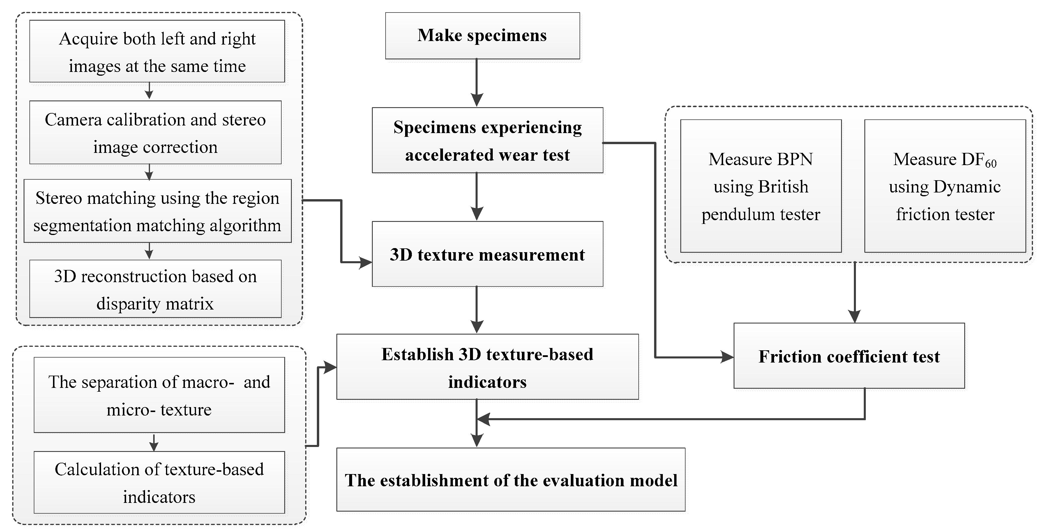
The research program includes the following steps: make specimens, specimens experiencing accelerated wear test, 3D texture measurement, establish 3D texture-based indicators, friction coefficient test and the establishment of evaluation model. The specific program is shown in Figure 1.
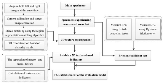
Figure 1.
The research program in this study.
4.1. Material Preparation
Four kinds of asphalt mixtures including AC-13, SMA-13, SMA-16, and OGFC-13 are selected. These mixtures respectively represent the different structure types: suspended dense type (AC-13), skeleton dense type (SMA-13 and SMA-16), and skeleton void type (OGFC-13). Additionally, three kinds of mineral aggregate containing limestone, basalt and steel slag are chosen for preparing each kind of asphalt mixture. The polished values of steel slag, basalt and limestone are respectively 67, 62 and 43 according to Chinese test standard T0345-2005. The abrasion resistance of steel slag is the best, then basalt, and limestone is the worst. Since the steel slag content with particle size more than 16 mm is very few, the asphalt mixture prepared by steel slag material do not contain SMA-16. AH70 oil bitumen with PG 64-22 whose pen grade is 60/80and I-C SBS modified asphalt with PG 70-22 were respectively selected as asphalt binder.
A total of 11 types of asphalt mixture are prepared, Table 1. Considering that the porous fine aggregate for steel slag will absorb more asphalt binder and thus raising the cost, the fine aggregate for steel slag material is replaced by basalt. In order to control the mixture gradation, different materials proportions have been used to achieve the principle of equal volume. The varying proportions will cause the difference in passing rate by weight between steel slag materials and limestone or basalt material. All asphalt mixture specimens are formed into plates with the size of 45 × 40 × 5 cm by wheel-roller compaction machine for further experiments.

Table 1.
Gradation composition of asphalt mixture specimens.
In order to acquire 3D texture and realize the establishment of model, each specimen needs to experience accelerated abrasion action before testing. The indoor accelerate abrasion tester manufactured in previous research is used [21]. In the first 6 h, the testing indicators of specimens are measured at 4 h and 6 h. Then the measurement is conducted every 4 h until the abrasion time reaches 38 h. For each asphalt mixture specimen, 10 sets of data need to be tested. The corresponding abrasion time is 4 h, 6 h, 10 h, 14 h, 18 h, 22 h, 26 h, 30 h, 34 h, and 38 h, respectively.
4.2. Measurement of Pavement 3D Texture
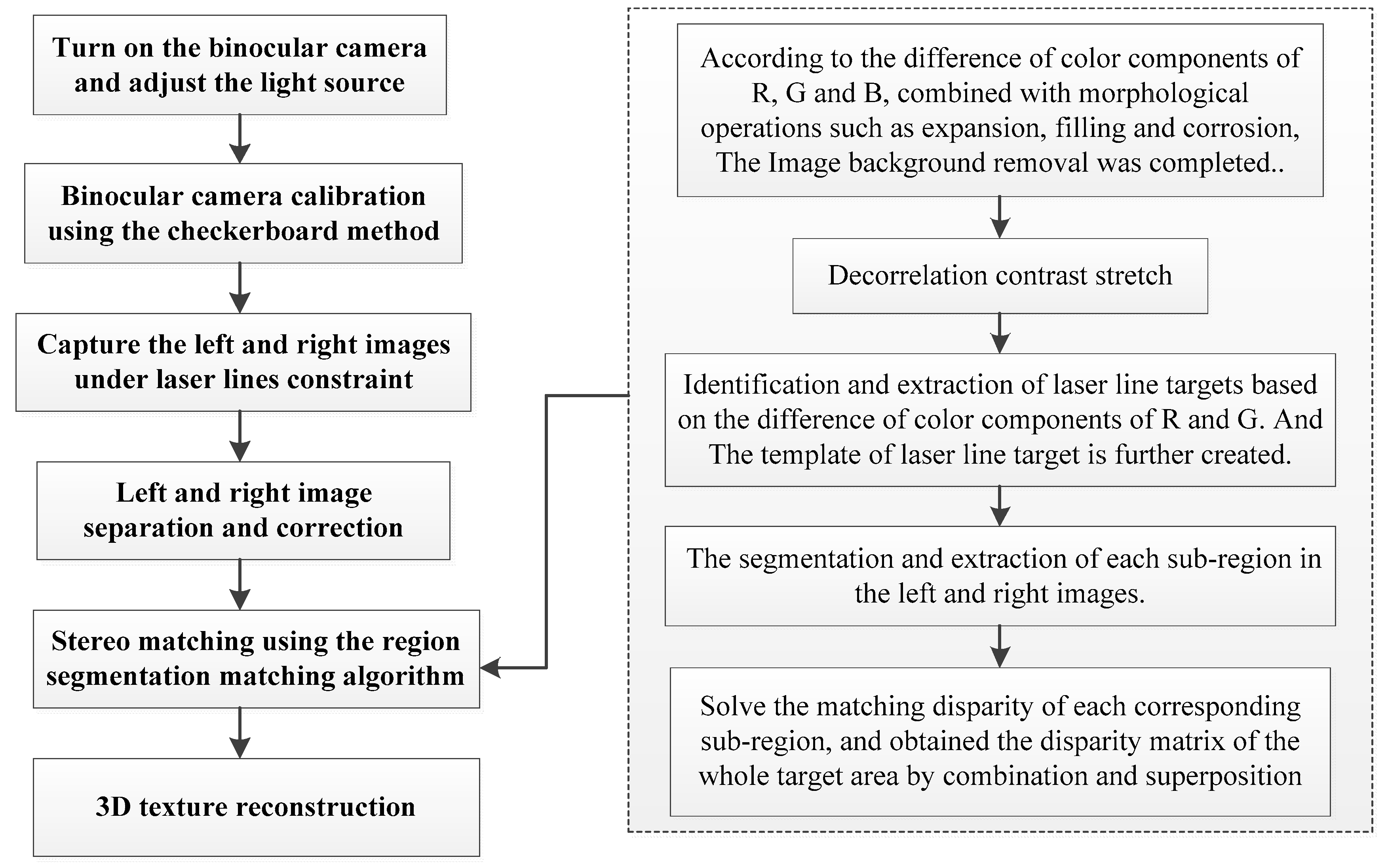
The improved binocular reconstruction method with six laser lines constraint is proposed to acquire both macro-texture and micro-texture. In this improved binocular reconstruction method, six laser lines are introduced to form mandatory matching and improve matching accuracy. The test system mainly composed of the binocular camera, the reinforcing light source, the linear laser transmitter and other components, Figure 2. In addition, the region segmentation matching algorithm is written to improve the traditional algorithm in the stereo matching process. In this matching algorithm, the target region is divided into seven sub-regions by six laser lines. The segmentation of sub-regions is completed based on the recognition of laser lines. Then, the disparity of each sub-region is solved and superimposed. Finally, 3D texture is obtained based on the superimposed disparity matrix. The specific test process is shown in Figure 3.
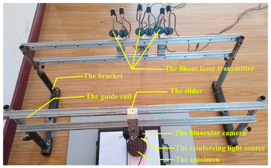
Figure 2.
The improved binocular reconstruction test system.
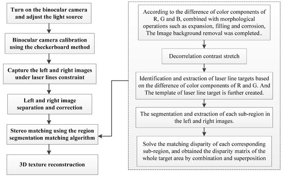
Figure 3.
The test flow chart of the improved binocular reconstruction method.
The whole test process is achieved through MATLAB programming. The average test accuracy of this improved method can reach 0.02 mm, which can meet the accuracy requirements of micro-texture measurement.
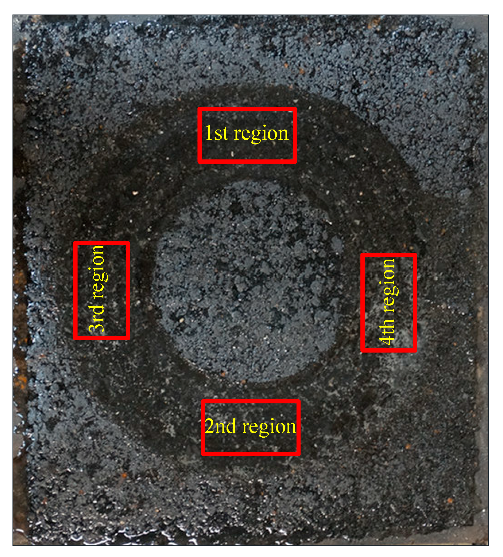
For every asphalt mixture specimen experiencing accelerated wear, four regions are collected to reconstruct the 3D texture, Figure 4. Each region’s area is 4.0 cm × 6.0 cm.

Figure 4.
The schematic diagram of 3D texture test area.
4.3. Establishment of 3D Texture-Based Indicators
After 3D texture extraction, the separation between macro-texture and micro-texture is necessary. Since the demarcation wavelength Δx between macro-texture and micro-texture is 0.5 mm, then the demarcation frequency F0, F0 = 1/(2Δx), is equal to 1 cycle/mm. When the demarcation frequency is known, the Gaussian low-pass filter is easily designed based on Fourier integral transform [22]. The radius of demarcation frequency of the low-pass filter d0 satisfies Equation (6).
where dx is the camera parameters; M, N are the size of images. Then d0 = 45, and the Gaussian low pass filtering can be determined. Based on the frequency domain transformation and the Gaussian low pass filtering, the separation between macro-texture and micro-texture is finally realized.
The results of mechanism analysis in the third section show that height, wavelength and shape characteristics can all affect the skid resistance. Therefore, 3D texture-based characterization indicators about these aspects are established respectively. The mean texture depth (MTD), the average spacing of single-peak (S), the root mean square wavelength (λ) and the skewness (Sk) are respectively used to describe pavement rough characteristics, Equations (7)–(10). The sign ‘1’ behind indicators is used to distinguish macro-texture from micro-texture. For example, MTD means THE MEAN TEXTURE DEPTH based on macro-texture; MTD1 is defined as the mean texture depth based on micro-texture.
where is the elevation of texture; is the horizontal coordinates; M and N are the numbers of sampling along X and Y directions; is the highest elevation of all points; p is the number of spacing of single-peak; Δx and Δy are respectively sampling interval; Si is ith spacing of adjacent single-peak. For the above characterization indicators, the test data will be abandoned if the relative deviation based on the average value is larger than 1.15 times of standard deviation. The average value is finally adopted.
4.4. Friction Coefficient Test
BPN and DF60 are respectively tested as the friction coefficient indicator through British pendulum tester and dynamic friction tester according to the test procedures [23,24]. The test area of BPN is the same with 3D texture. While the test areas of DF60 is a ring with a diameter of 30 cm that is along the track of the accelerate abrasion tester. BPN and DF60 represent the skid resistance of the road under different conditions. BPN is a quasi-static index, which represents the anti-skid performance of road under low speed driving conditions. DF60 is a dynamic index, which reflects the anti-skid performance of a road with a high driving speed.
5. Results and Discussion
5.1. The model Analysis Based on 3D Texture Data
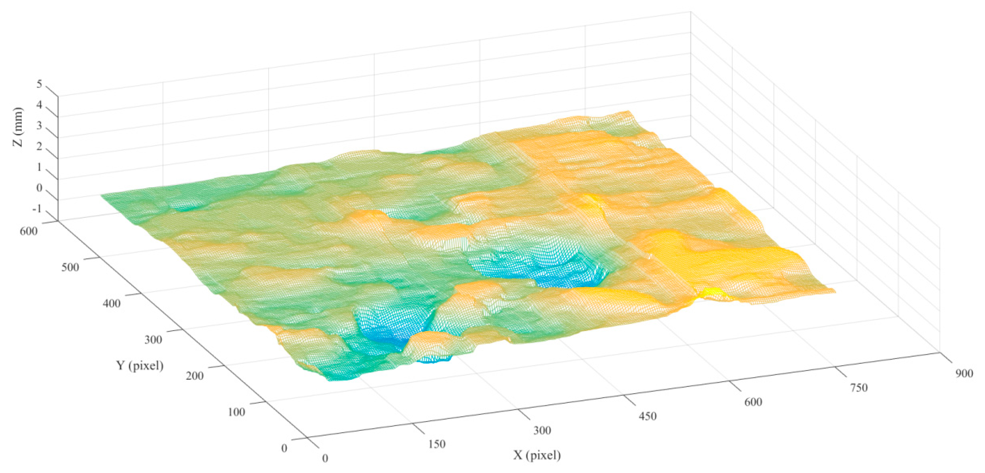
According to the research program, the 3D texture and the friction coefficients of each specimen are respectively tested. Then, a total of 110 sets of data are obtained. However, only the test data of AC-13 using limestone is shown in Table 2. The 3D texture reconstruction results of AC-13(L)-4 h are displayed in Figure 5.
Table 2.
The test data of AC-13.
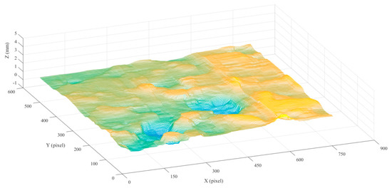
Figure 5.
The 3D texture reconstruction results of AC-13(L)-4h.
The multiple linear regression model is first used to analyze the relationship between pavement skid resistance (BPN, DF60) and 3D texture indicators. Regrettably, the Regression coefficient R2 is relatively low, no more than 0.5. Thus, the multiple linear regression model is unsuitable for the relationship building. Therefore, the other regression model will be further considered.
Then the multiple quadratic multinomial regression model is used. 3D texture-based indicators are firstly integrated into a synthetic vector: . X and Y are the virtual variables, which represent the wear resistance of aggregates. X = 1 means the mineral aggregate is limestone; X = 0 means the mineral aggregate is other materials. When X = 0 and Y = 1, the mineral aggregate is steel slag; but when X = 0 and Y = 0, then the mineral aggregate is basalt. The model can be expressed as follows:
where, F is the skid resistance indicator (it refers to BPN or DF60 in this article); M is the synthetic vector; A, B and C are respectively the quadratic term coefficient matrix, monomial coefficient matrix and the constant term. The matrix A is a symmetric square matrix.
The statistical analysis software (SAS) is used to write programs for solving this regression model. Then the insignificant independent variables are removed in turn by stepwise analysis until obtaining a satisfactory regression effect. One favorable regression effect is mainly reflected in three aspects: First, the fitting degree is excellent, namely that the value of R2 is close to 1; Second, model equation satisfies the significant level, which means the inspection probability of model parameter estimation satisfies: p < 0.05; Third, there is a significant regression relationship between all independent variables and dependent variable. The probability of factor test satisfies: p < 0.05.
As for the regression model of BPN, four indicators (X, MTD1, Sk1 and λ) are finally retained to constitute the synthetic vector: . The regression analysis results are shown in Table 3, Table 4 and Table 5. Then, the multiple quadratic multinomial regression model and the parameters A1, B1 and C1 are shown in Equation (12).
Table 3.
Summary results of final BPN model.
Table 4.
The inspection of final BPN model parameters estimation.
Table 5.
Factor test results of final BPN model.
In Table 3, the R2 is 0.8035. Data points are more densely gathered near the regression estimation, which means the fitting degree is good. In Table 4, All the probability values of linear, quadratic, crossproduct and total model are lower than 0.05. The relationship between dependent variable and independent variables is significant, and the regression equation model is also significant. Additionally, a factor test of model independent variables is further processed, shown in Table 5. The probability values are all smaller than 0.05, which indicate that the overall regression coefficient of each factor is highly significant.
As for the regression model of DF60, five indicators X, Y, MTD, Sk1 and λ are finally retained to constitute the synthetic vector M2. Then the multiple quadratic polynomial model between DF60 and M2 is established. The regression analysis results are shown in Table 6, Table 7 and Table 8, and the multiple quadratic multinomial regression equation and the parameters A2, B2 and C2 are shown in Equation (13).
Table 6.
Summary results of final DF60 model.
Table 7.
The estimate inspection of final DF60 model parameters.
Table 8.
Factor test results of final DF60 model.
In Table 6, R2 is as high as 0.9255 and root MES is only 0.0251. The fitting degree is high. Notably, the total data points can well gather near the regression estimation. The F test-based probability values of linear, quadratic, crossproduct, and total model are respectively listed in Table 7. Although the probability value of quadratic cannot meet the requirements of below 0.05, the probability value of total model satisfies p < 0.0001. From the perspective of overall level, the regression equation model is significant. Additionally, the significant degree of regression coefficient is provided in Table 8. The results show that the probability values of every factor are all lower than 0.05, which means that the overall regression coefficient of each factor is highly significant.
The comparison between Equations (12) and (13) indicates that the independent variable Y appears in DF60 model but not in BPN model. The results show that compared with DF60, the requirements of mineral aggregate classification for BPN model is relative loose. Analyzing the reasons maybe that different testing speeds determine the impact and abrasion of test equipment on aggregates. Then more intense forces make DF60 more sensitive to the hardness or wear-resistant of mineral aggregates.
5.2. The Further Harmonization of Evaluation Model
At present, there are numerous types of equipment being used to test pavement skid resistance. And the evaluation standard from different test methods is not unified, which brings a lot of obstacles for the communication with each other. In order to harmonize different test methods, the Permanent International Association of Road Congresses (PIARC) proposed the PIARC model and established International Friction Index (IFI). IFI was defined as the function containing two parameters Sp and F60. In IFI evaluation method, F(S) can be calculated:
where, F(S) is the standard friction coefficient at any testing speed S; F60 is the standard friction number, which can be calculated from the friction coefficient tested by any detection equipment at any testing speed FRS; Sp is the speed number, which represents the morphological characteristics of macro-texture.
The relationship between Sp and MTD has been listed in the references [25,26]. The calibration parameters of F60 corresponding to DF60 have also been given in the reference (ASTM, 2011), Equations (15) and (16).
In Section 5.1, the relational expression between DF60 and 3D texture indicators has been established. Then, the harmonization of evaluation model using 3D texture data can be obtained easily, in Equation (17).
In Equation (16), the final evaluation model just needs to measure the pavement 3D texture. It is no longer necessary to test the friction coefficient in field environment that has strong conditional limitations. After testing pavement 3D texture, it directly calculates the standard friction coefficient at any testing speed F(S). Then, FRS tested by any detection equipment at any testing speed can be solved through F60. Hence, the harmonization and comparison from different test methods can be easily achieved based on the evaluation model. In summary, this evaluation model is simple to operate and implement, since the evaluation results directly depend on pavement 3D texture. It also combines with the advantages of IFI evaluation method, which is conducive to harmonize different testing results from different detection conditions.
6. Conclusions
In this study, the evaluation model of pavement skid resistance using 3D texture data is proposed and established through the multiple quadratic multinomial regression model. The following conclusions can be drawn.
The mechanism of pavement skid resistance based on macro-texture and micro-texture is analyzed. The results show that the macro-texture directly affects the hysteresis component of friction. Especially, the macro-texture can increase the drainage capability and improve skid resistance during rainy driving. As for micro-texture, it mainly affects the adhesive component of friction. No matter whether macro-texture or micro-texture, the texture characteristics such as height, wavelength, and shape can all affect the pavement skid resistance.
The improved binocular reconstruction method with six laser lines constraint is used to acquire both macro-texture and micro-texture. The 3D texture-based indicators involving more characteristics are further used to establish the evaluation model. The results indicate that the fitting degree, parameter estimation test and factor test all indicate that multiple quadratic multinomial regression model can well describe the relationship between friction coefficients and 3D texture. It has a higher fitting degree and significant model relationship.
In order to harmonize different detection methods, the evaluation model of skid resistance using 3D texture data is established. This proposed evaluation model can not only combine with the advantages of IFI, but also avoid the measurement of friction coefficient owning strong conditional restrictions. This evaluation model provides a new approach for evaluating pavement skid resistance, whose evaluation results directly depend on pavement 3D texture and aggregate types.
Although the proposed model has achieved satisfactory test results, there are still the following aspects to be considered: Only three kinds of aggregates are used in experiment process. The effect of more kinds of aggregates on the evaluation model needs to be further studied; the results and analyses provided in this paper are only based on this laboratory experiment scenario. However, these results may not be completely valid for field conditions. Further, similar study on the comparison between laboratory simulation and field conditions is accordingly needed.
Author Contributions
Conceptualization, Y.W. and F.Z.; methodology, Y.W. and J.X.; software, Y.W. and X.L.; validation, F.Z.; formal analysis, Y.W.; investigation, Y.W. and X.L.; resources, Y.W.; data curation, Y.W. and X.L.; writing—original draft preparation, Y.W.; writing—review and editing, Y.W., F.Z. and J.X.; visualization, Y.W.; supervision, F.Z.; project administration, F.Z.; funding acquisition, Y.W. All authors have read and agreed to the published version of the manuscript.
Funding
This research was funded by the National Natural Science Foundation of China (51808084), the Project of Hubei University of Arts and Science (XK2019065) and Doctoral Research Foundation of Hubei University of Arts and Science (2059047), to which the authors are grateful.
Conflicts of Interest
There is no conflict of interest.
References
- National Bureau of Statistics. The statistical bulletin of the people’s republic of China on national economic and social development in 2016. People’s Daily, 1 March 2017; 010. [Google Scholar]
- NHTSA (National Highway Traffic Safety Administration). 2015 Motor Vehicle Crashes: Overview, Washington, DC. 2016. Available online: https://crashstats.nhtsa.dot.gov/Api/Public/ViewPublication/812318 (accessed on 23 December 2017).
- Claeys, X.; Yi, J.; Alvarez, L.; Horowitz, R.; Richard, L. Tire friction modeling under wet road conditions. In Proceedings of the American Control Conference, Arlington, VA, USA, 25–27 June 2001; IEEE: Piscataway, NJ, USA, 2001. [Google Scholar]
- Hosking, J.R. Relationship between Skidding Resistance and Accident Frequency: Estimates Based on Seasonal Variation. Research Report 76; Transport and Road Research Laboratory (TRRL), Department of Transport: Crowthorne, UK, 1987. [Google Scholar]
- Saito, K.; Horiguchi, T.; Kasahara, A.; Abe, H.; Henry, J.J. Development of portable tester for measuring skid resistance and its speed dependency on pavement surfaces. Transp. Res. Rec. 1996, 1536, 45–51. [Google Scholar] [CrossRef]
- Bijsterveld, W.; Val, M. Towards quantification of seasonal variations in skid resistance measurements. Road Mater. Pavement Des. 2016, 17, 477–486. [Google Scholar] [CrossRef]
- Tan, T.; Xing, C.; Tan, Y.; Gong, X. Safety aspects on icy asphalt pavement in cold region through field investigations. Cold Reg. Sci. Technol. 2019, 161, 21–31. [Google Scholar] [CrossRef]
- Wu, J.; Zhang, C.; Wang, Y.; Su, B.; Gond, B. Investigation on Wet Skid Resistance of Tread Rubber. Exp. Tech. 2019, 43, 81–89. [Google Scholar] [CrossRef]
- Panagouli, O.K.; Kokkalis, A.G. Skid resistance and fractal structure of pavement surface. Chaos Solitons Fractals 1998, 9, 493–505. [Google Scholar] [CrossRef]
- Choubane, B.; Holzschuher, C.; Gokhale, S. Precision of locked-wheel testers for measurement of roadway surface friction characteristics. Transp. Res. Rec. 2004, 1869, 145–151. [Google Scholar] [CrossRef]
- World Road Association. PIARC Report of the Committee on Surface Characteristics. In Proceedings of the XVIII World Road Congress, Brussels, Belgium, 13–19 September 1987. [Google Scholar]
- Xie, X.; Lu, G.; Liu, P.; Zhou, Y.; Wang, D.; Oeser, M. Influence of temperature on polishing behaviour of asphalt road surfaces. Wear 2018, 402, 49–56. [Google Scholar] [CrossRef]
- Yang, G.; Li, Q.J.; Zhan, Y.; Fei, Y.; Zhang, A. Convolutional Neural Network–Based Friction Model Using Pavement Texture Data. J. Comput. Civil Eng. 2018, 32, 04018052. [Google Scholar] [CrossRef]
- Kogbara, R.B.; Masad, E.A.; Woodward, D.; Millar, P. Relating surface texture parameters from close range photogrammetry to Grip-Tester pavement friction measurements. Constr. Build. Mater. 2018, 166, 227–240. [Google Scholar] [CrossRef]
- Rezaei, A.; Masad, E.; Chowdhury, A. Development of a model for asphalt pavement skid resistance based on aggregate characteristics and gradation. J. Transp. Eng. 2011, 137, 863–873. [Google Scholar] [CrossRef]
- Tabor, D. Friction—The present state of our understanding. J. Tribol. 1981, 103, 169–179. [Google Scholar] [CrossRef]
- Moore, D.F. The Friction of Pneumatic Tyres; Elsevier Scientific Publishing Co.: New York, NY, USA, 1975. [Google Scholar]
- Cao, P. Study on Effects of Texture and Contaminants to Skid Resistance of Asphalt Pavements. Ph.D. Thesis, Wuhan University of Technology, Wuhan, China, 2009. (In Chinese). [Google Scholar]
- Smith, N.F. Bernoulli and Newton in fluid mechanics. Phys. Teach. 1972, 10, 451–455. [Google Scholar] [CrossRef]
- Dai, Q. Study on the Influence of Asphalt Pavement Surface Characteristic on Skid Resistance. Master’s Thesis, Southeast University, Nanjing, China, 2007. (In Chinese). [Google Scholar]
- Wang, Y.Y.; Yang, Z.; Liu, Y.; Sun, L. The characterisation of three-dimensional texture morphology of pavement for describing pavement sliding resistance. Road Mater. Pavement Des. 2019, 20, 1076–1095. [Google Scholar] [CrossRef]
- Gunaratne, M.; Bandara, N.; Medzorian, J.; Chawla, M.; Ulrich, P. Correlation of tire wear and friction to texture of concrete pavements. J. Mater. Civil Eng. 2000, 12, 46–54. [Google Scholar] [CrossRef]
- ASTM. Standard Test. Method for Measuring Surface Frictional Properties Using the British Pendulum Tester. ASTM E303-93; ASTM: West Conshohocken, PA, USA, 2013. [Google Scholar]
- ASTM. Standard Test. Method for Measuring Paved Surface Frictional Properties Using the Dynamic Friction Tester. ASTM E1911-09; ASTM: West Conshohocken, PA, USA, 2009. [Google Scholar]
- ASTM. Standard Test. Method for Measuring Pavement Macrotexture Properties Using the Circular Track Meter. ASTM E2157-09; ASTM: West Conshohocken, PA, USA, 2009. [Google Scholar]
- ASTM. Standard Practice for Calculating the International Friction Index of a Pavement Surface. ASTM E2100-07; ASTM: West Conshohocken, PA, USA, 2011. [Google Scholar]

© 2020 by the authors. Licensee MDPI, Basel, Switzerland. This article is an open access article distributed under the terms and conditions of the Creative Commons Attribution (CC BY) license (http://creativecommons.org/licenses/by/4.0/).