
The Wavelet Transform for Feature Extraction and Surface Roughness Evaluation after Micromachining


Abstract
:1. Introduction
2. Detection of Measurement Noise
Noise Extraction Method Based on Subtraction of Random Variables
3. Examination of Adaptive Wavelet Filtering
3.1. Examination of Adaptive Filtration Method Using Mathematical Formulae
3.1.1. SGPs of the Analytically Generated Roughness Profile of the Ideal Surface
3.1.2. SGPs of the Discretized Roughness Profile of the Ideal Surface
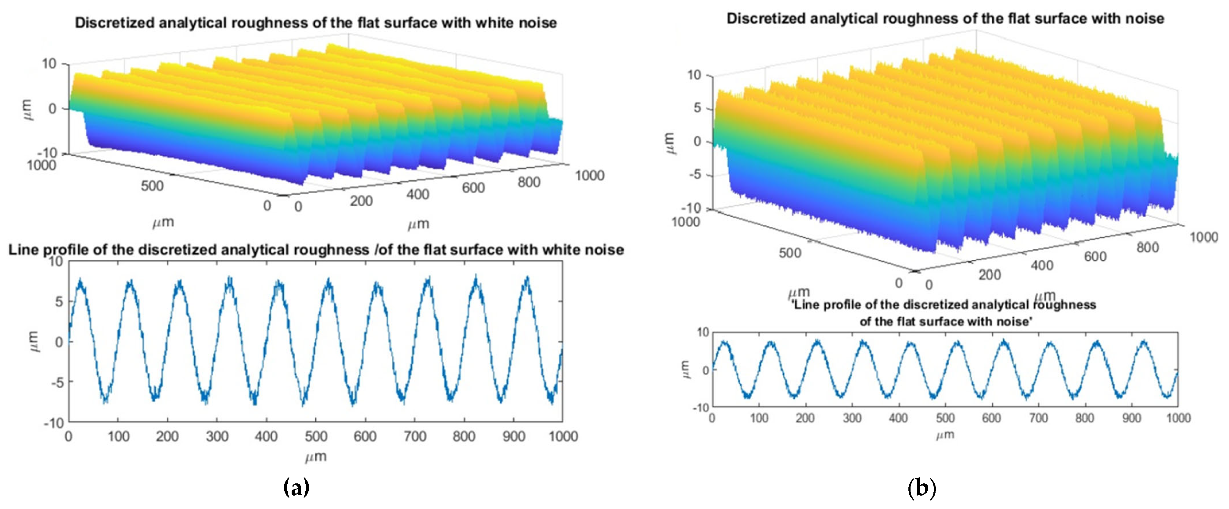
3.1.3. SGPs of the Discretized Roughness Profile with Simulated Measurement Noise
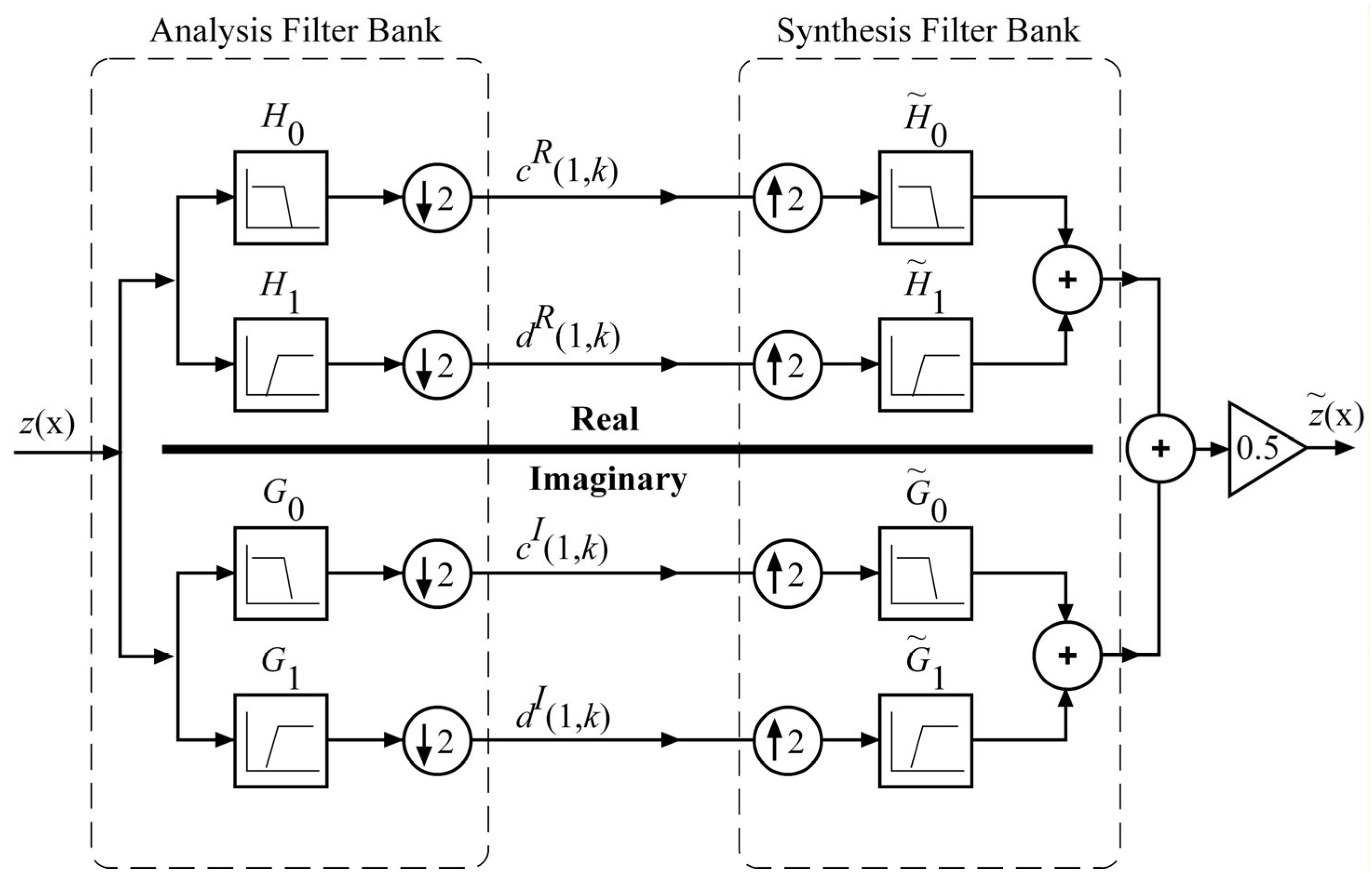
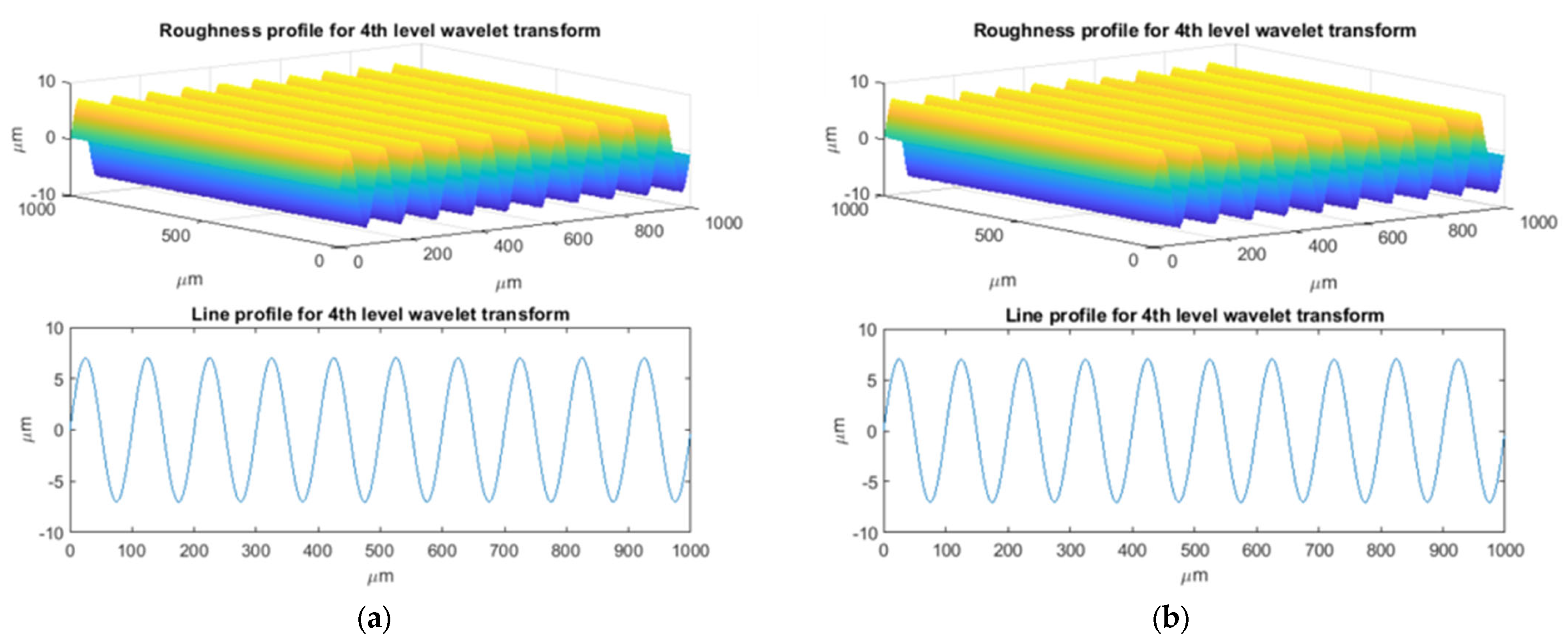
3.1.4. Proposed Method of SGP Calculation Based on Wavelet Analysis
3.2. Examination of Adaptive Filtration Method Using a Material Standard of Roughness
4. Discussion on SGP Calculation Method Based on Wavelet Analysis and Subtraction of Random Variables
5. Conclusions
- The best method to remove measurement noise from small areas is to use wavelet filtering based on minimization of RMS of the signal (the values of Sq of the filtered rest). This filtration method allows the separation of noise in individual measurements (where values are the same). Additionally, it was proven with analytical methods, which were confirmed in practice, that the wavelet filtering method that uses so-called Kinsburry dual-tree complex wavelet transform can very well remove noise from small surface areas (without deforming the surface, as is the case in Gaussian filtering).
- It can be assumed that technological surfaces of random (isotropic/anisotropic) morphology of any size XY and any resolution can be filtered with wavelet transform based on RMS signal minimization. However, during experiments it is important. The above observations require further experimental research. It remains to be checked whether the application of wavelet filtering can result in “defiltering” of unique surface features (such as tribological, hydrophobic, or hydrophilic properties).
- Wavelet filtering can reduce the spread of surface geometry parameters. It is crucial when deciding which would enable unequivocal assessment of an object (especially when the value of the parameter under investigation is on the borderline: good/not good). In this way, the likelihood of escalating problems in the industry can be reduced.
- Of the many methods for removing noise (errors of the measuring apparatus), the Kinsburry wavelet works best, and this is true regardless of the surface area and resolution adopted when scanning the surface. Once this phenomenon was explained, it was possible to use the developed filtering method and wavelet filter optimization in surface micromachining research. The results may be useful in other areas of technology and life sciences.
Author Contributions
Funding
Institutional Review Board Statement
Informed Consent Statement
Data Availability Statement
Acknowledgments
Conflicts of Interest
References
- Grzejda, R. Modelling Nonlinear Multi-Bolted Connections: A Case of Operational Condition. In Proceedings of the 15th International Scientific Conference ‘Engineering for Rural Development 2016’, Jelgava, Latvia, 25–27 May 2016; pp. 336–341. [Google Scholar]
- Grzejda, R. New method of modelling nonlinear multi-bolted systems. In Advances in Mechanics: Theoretical, Computational and Interdisciplinary Issues, 1st ed.; Kleiber, M., Burczyński, T., Wilde, K., Gorski, J., Winkelmann, K., Smakosz, Ł., Eds.; CRC Press: Leiden, The Netherlands, 2016; pp. 213–216. [Google Scholar]
- Palenica, P.; Powałka, B.; Grzejda, R. Assessment of modal parameters of a building structure model. Springer Proc. Math. Stat. 2016, 181, 319–325. [Google Scholar]
- Ba, Z.; Wang, Y.; Sun, T.; Jia, Y.; Zhang, L.; Dong, Q. Preparation and properties of hydrophobic micro-arc oxidation/layered double hydroxide composite coating on magnesium alloy. Surf. Coat. Technol. 2023, 475, 130113. [Google Scholar] [CrossRef]
- Kumar, S.S.A.; Ma, I.A.W.; Ramesh, K.; Ramesh, S. The synergistic effects of graphene on the physical, hydrophobic, surface, and thermal properties of acrylic-epoxy-polydimethylsiloxane composite coatings. Int. J. Adhes. Adhes. 2024, 128, 103546. [Google Scholar] [CrossRef]
- Brinksmeier, E.; Preuss, W. Micro-machining. Philos. Trans. R. Soc. A Math. Phys. Eng. Sci. 2012, 370, 3973–3992. [Google Scholar] [CrossRef] [PubMed]
- Chen, T.-H.; Fardel, R.; Arnold, C.B. Ultrafast z-scanning for high-efficiency laser micro-machining. Light Sci. Appl. 2018, 7, 17181. [Google Scholar] [CrossRef] [PubMed]
- Wan, M.; Wen, D.-Y.; Ma, Y.-C.; Zhang, W.-H. On material separation and cutting force prediction in micro milling through involving the effect of dead metal zone. Int. J. Mach. Tools Manuf. 2019, 146, 103452. [Google Scholar] [CrossRef]
- Aslantas, K.; Danish, M.; Hasçelik, A.; Mia, M.; Gupta, M.; Ginta, T.; Ijaz, H. Investigations on surface roughness and tool wear characteristics in micro-turning of Ti-6Al-4V alloy. Materials 2020, 13, 2998. [Google Scholar] [CrossRef] [PubMed]
- Aurich, J.C.; Engmann, J.; Schueler, G.M.; Haberland, R. Micro grinding tool for manufacture of complex structures in brittle materials. CIRP Ann. 2009, 58, 311–314. [Google Scholar] [CrossRef]
- Kumar, S.P.L. Measurement and uncertainty analysis of surface roughness and material removal rate in micro turning operation and process parameters optimization. Measurement 2019, 140, 538–547. [Google Scholar] [CrossRef]
- Setti, D.; Arrabiyeh, P.A.; Kirsch, B.; Heintz, M.; Aurich, J.C. Analytical and experimental investigations on the mechanisms of surface generation in micro grinding. Int. J. Mach. Tools Manuf. 2020, 149, 103489. [Google Scholar] [CrossRef]
- Lee, P.-H.; Nam, J.S.; Li, C.; Lee, S.W. An experimental study on micro-grinding process with nanofluid minimum quantity lubrication (MQL). Int. J. Precis. Eng. Manuf. 2012, 13, 331–338. [Google Scholar] [CrossRef]
- Guo, J.; Suzuki, H.; Higuchi, T. Development of micro polishing system using a magnetostrictive vibrating polisher. Precis. Eng. 2013, 37, 81–87. [Google Scholar] [CrossRef]
- Nüsser, C.; Wehrmann, I.; Willenborg, E. Influence of intensity distribution and pulse duration on laser micro polishing. Phys. Procedia 2011, 12, 462–471. [Google Scholar] [CrossRef]
- Chavoshi, S.Z.; Luo, X. Hybrid micro-machining processes: A review. Precis. Eng. 2015, 41, 1–23. [Google Scholar] [CrossRef]
- Flucke, C.; Gläbe, R.; Brinksmeier, E. Diamond Micro Chiseling: Cutting of Prismatic Micro Optic Arrays. In Proceedings of the 7th International Conference—European Society for Precision Engineering and Nanotechnology, Bremen, Germany, 20–24 May 2007. [Google Scholar]
- PN-EN ISO 16610-21; Geometrical Product Specifications (GPS), Filtration, Part 21: Linear Profile Filters: Gaussian Filters. Polish Committee for Standardization: Warsaw, Poland, 2013.
- PN-EN ISO 16610-22; Geometrical Product Specifications (GPS), Filtration, Part 22: Linear Profile Filters: Spline Filters. Polish Committee for Standardization: Warsaw, Poland, 2015.
- PN-EN ISO 16610-28; Geometrical Product Specifications (GPS), Filtration, Part 28: Profile Filters: End Effects. Polish Committee for Standardization: Warsaw, Poland, 2017.
- PN-EN ISO 16610-29; Geometrical Product Specifications (GPS), Filtration, Part 29: Linear Profile Filters: Wavelets. Polish Committee for Standardization: Warsaw, Poland, 2020.
- PN-EN ISO 16610-31; Geometrical Product Specifications (GPS), Filtration, Part 31: Robust Profile Filters: Gaussian Regression Filters. Polish Committee for Standardization: Warsaw, Poland, 2017.
- PN-EN ISO 16610-41; Geometrical Product Specifications (GPS), Filtration, Part 41: Morphological Profile Filters: Disk and Horizontal Line-Segment Filters. Polish Committee for Standardization: Warsaw, Poland, 2015.
- PN-EN ISO 16610-49; Geometrical Product Specifications (GPS), Filtration, Part 49: Morphological Profile Filters: Scale Space Techniques. Polish Committee for Standardization: Warsaw, Poland, 2015.
- PN-EN ISO 16610-61; Geometrical Product Specifications (GPS), Filtration, Part 61: Linear Areal Filters: Gaussian Filters. Polish Committee for Standardization: Warsaw, Poland, 2015.
- PN-EN ISO 16610-62; Geometrical Product Specifications (GPS), Filtration, Part 62: Linear Areal Filters: Spline Filters. Polish Committee for Standardization: Warsaw, Poland, 2023.
- PN-EN ISO 16610-71; Geometrical Product Specifications (GPS), Filtration, Part 71: Robust Areal Filters: Gaussian Regression Filters. Polish Committee for Standardization: Warsaw, Poland, 2015.
- PN-EN ISO 16610-85; Geometrical Product Specifications (GPS), Filtration, Part 85: Morphological Areal Filters: Segmentation. Polish Committee for Standardization: Warsaw, Poland, 2013.
- Whitehouse, D.J. Handbook of Surface Metrology, 1st ed.; CRC Press: New York, NY, USA, 1994. [Google Scholar]
- Dobrzanski, P.; Pawlus, P. Digital filtering of surface topography: Part I. Separation of one-process surface roughness and waviness by Gaussian convolution, Gaussian regression and spline filters. Precis. Eng. 2010, 34, 647–650. [Google Scholar] [CrossRef]
- Kondo, Y.; Yoshida, I.; Nakaya, D.; Numada, M.; Koshimizu, H. Verification of characteristics of Gaussian filter series for surface roughness in ISO and proposal of filter selection guidelines. Nanomanuf. Metrol. 2021, 4, 97–108. [Google Scholar] [CrossRef]
- PN-EN ISO 3274; Geometrical Product Specifications (GPS), Surface Texture: Profile Method, Nominal Characteristics of Contact (Stylus) Instruments. Polish Committee for Standardization: Warsaw, Poland, 2011.
- Wang, Z.; Meng, H.; Fu, J. Novel method for evaluating surface roughness by grey dynamic filtering. Measurement 2010, 43, 78–82. [Google Scholar] [CrossRef]
- Le Goïc, G.; Bigerelle, M.; Samper, S.; Favrelière, H.; Pillet, M. Multiscale roughness analysis of engineering surfaces: A comparison of methods for the investigation of functional correlations. Mech. Syst. Signal Process. 2016, 66–67, 437–457. [Google Scholar] [CrossRef]
- Eseholi, T.; Coudoux, F.-X.; Corlay, P.; Sadli, R.; Bigerelle, M. A multiscale topographical analysis based on morphological information: The HEVC multiscale decomposition. Materials 2020, 13, 5582. [Google Scholar] [CrossRef]
- He, B.; Zheng, H.; Ding, S.; Yang, R.; Shi, Z. A review of digital filtering in evaluation of surface roughness. Metrol. Meas. Syst. 2021, 28, 217–253. [Google Scholar] [CrossRef]
- Pérez-Ruiz, J.D.; de Lacalle, L.N.L.; Urbikain, G.; Pereira, O.; Martínez, S.; Bris, J. On the relationship between cutting forces and anisotropy features in the milling of LPBF Inconel 718 for near net shape parts. Int. J. Mach. Tools Manuf. 2021, 170, 103801. [Google Scholar] [CrossRef]
- Pérez-Ruiz, J.D.; Marin, F.; Martínez, S.; Lamikiz, A.; Urbikain, G.; de Lacalle, L.N.L. Stiffening near-net-shape functional parts of Inconel 718 LPBF considering material anisotropy and subsequent machining issues. Mech. Syst. Signal Process. 2022, 168, 108675. [Google Scholar] [CrossRef]
- Matuszak, M.; Garbellini, A.; Powałka, B.; Attanasio, A.; Bachtiak-Radka, E. Accuracy analysis of the micro-milling process. J. Mach. Constr. Maint. 2017, 107, 37–43. [Google Scholar]
- Pour, M. Determining surface roughness of machining process types using a hybrid algorithm based on time series analysis and wavelet transform. Int. J. Adv. Manuf. Technol. 2018, 97, 2603–2619. [Google Scholar] [CrossRef]
- Lucas, K.; Sanz-Lobera, A.; Antón-Acedos, P.; Amatriain, A. A survey of bidimensional wavelet filtering in surface texture characterization. Procedia Manuf. 2019, 41, 811–818. [Google Scholar] [CrossRef]
- Zmarzły, P. Influence of bearing raceway surface topography on the level of generated vibration as an example of operational heredity. Indian J. Eng. Mater. Sci. 2020, 27, 356–364. [Google Scholar]
- Prabhakar, D.V.N.; Kumar, M.S.; Krishna, A.G. A Novel Hybrid Transform approach with integration of Fast Fourier, Discrete Wavelet and Discrete Shearlet Transforms for prediction of surface roughness on machined surfaces. Measurement 2020, 164, 108011. [Google Scholar] [CrossRef]
- Gogolewski, D. Fractional spline wavelets within the surface texture analysis. Measurement 2021, 179, 109435. [Google Scholar] [CrossRef]
- Dutta, S.; Pal, S.K.; Sen, R. Progressive tool flank wear monitoring by applying discrete wavelet transform on turned surface images. Measurement 2016, 77, 388–401. [Google Scholar] [CrossRef]
- Wang, X.; Shi, T.; Liao, G.; Zhang, Y.; Hong, Y.; Chen, K. Using wavelet packet transform for surface roughness evaluation and texture extraction. Sensors 2017, 17, 933. [Google Scholar] [CrossRef]
- Sun, J.; Song, Z.; He, G.; Sang, Y. An improved signal determination method on machined surface topography. Precis. Eng. 2018, 51, 338–347. [Google Scholar] [CrossRef]
- Josso, B.; Burton, D.R.; Lalor, M.J. Frequency normalised wavelet transform for surface roughness analysis and characterisation. Wear 2002, 252, 491–500. [Google Scholar] [CrossRef]
- Zahouani, H.; Mezghani, S.; Vargiolu, R.; Dursapt, M. Identification of manufacturing signature by 2D wavelet decomposition. Wear 2008, 264, 480–485. [Google Scholar] [CrossRef]
- Gogolewski, D.; Makieła, W.; Stępień, K.; Zmarzły, P.; Wrzochal, M. The Assessment of Wavelet Transform Parameters Regarding its Use in 3D Surface Filtering. In Proceedings of the 29th DAAAM International Symposium on Intelligent Manufacturing and Automation, Zadar, Croatia, 24–27 October 2018; pp. 1191–1196. [Google Scholar]
- Shao, Y.; Du, S.; Tang, H. An extended bi-dimensional empirical wavelet transform based filtering approach for engineering surface separation using high definition metrology. Measurement 2021, 178, 109259. [Google Scholar] [CrossRef]
- Daffara, C.; Mazzocato, S.; Marchioro, G. Multiscale roughness analysis by microprofilometry based on conoscopic holography: A new tool for treatment monitoring in highly reflective metal artworks. Eur. Phys. J. Plus 2022, 137, 430. [Google Scholar] [CrossRef]
- Beck, T.W.; DeFreitas, J.M.; Cramer, J.T.; Stout, J.R. A comparison of adaptive and notch filtering for removing electromagnetic noise from monopolar surface electromyographic signals. Physiol. Meas. 2009, 30, 353. [Google Scholar] [CrossRef]
- Lu, G.; Brittain, J.-S.; Holland, P.; Yianni, J.; Green, A.L.; Stein, J.F.; Aziz, T.Z.; Wang, S. Removing ECG noise from surface EMG signals using adaptive filtering. Neurosci. Lett. 2009, 462, 14–19. [Google Scholar] [CrossRef]
- Lou, S.; Tang, D.; Zeng, W.; Zhang, T.; Gao, F.; Muhamedsalih, H.; Jiang, X.; Scott, P.J. Application of clustering filter for noise and outlier suppression in optical measurement of structured surfaces. IEEE Trans. Instrum. Meas. 2020, 69, 6509–6517. [Google Scholar] [CrossRef]
- Podulka, P. Reduction of influence of the high-frequency noise on the results of surface topography measurements. Materials 2021, 14, 333. [Google Scholar] [CrossRef]
- Li, Z.; Gröger, S. Investigation of noise in surface topography measurement using structured illumination microscopy. Metrol. Meas. Syst. 2021, 28, 767–779. [Google Scholar] [CrossRef]
- PN-EN ISO 25178-2; Geometrical Product Specifications (GPS), Surface Texture: Areal, Part 2: Terms, Definitions and Surface Texture Parameters. Polish Committee for Standardization: Warsaw, Poland, 2022.
- Grochała, D.; Berczyński, S.; Grządziel, Z. Analysis of surface geometry changes after hybrid milling and burnishing by ceramic ball. Materials 2019, 12, 1179. [Google Scholar] [CrossRef] [PubMed]
- Rodriguez, A.; de Lacalle, L.N.L.; Pereira, O.; Fernandez, A.; Ayesta, I. Isotropic finishing of austempered iron casting cylindrical parts by roller burnishing. Int. J. Adv. Manuf. Technol. 2020, 110, 753–761. [Google Scholar] [CrossRef] [PubMed]
- Pappas, A.; Newton, L.; Thomson, A.; Hooshmand, H.; Leach, R. Uncertainty Propagation of Field Areal Surface Texture Parameters Using the Metrological Characteristics Approach. In Proceedings of the EuSPEN’s 23rd International Conference & Exhibition, Copenhagen, Denmark, 12–16 June 2023. [Google Scholar]
- Selesnick, I.W.; Baraniuk, R.G.; Kingsbury, N.C. The dual-tree complex wavelet transform. IEEE Signal Process. Mag. 2005, 22, 123–151. [Google Scholar] [CrossRef]
- Jiang, X.; Scott, P.; Whitehouse, D. Wavelets and their applications for surface metrology. CIRP Ann. 2008, 57, 555–558. [Google Scholar] [CrossRef]
- Whitehouse, D.J. Handbook of Surface and Nanometrology, 2nd ed.; CRC Press: Boca Raton, FL, USA, 2011. [Google Scholar]
- García Plaza, E.; Núñez López, P.J. Application of the wavelet packet transform to vibration signals for surface roughness monitoring in CNC turning operations. Mech. Syst. Signal Process. 2018, 98, 902–919. [Google Scholar] [CrossRef]
- Donoho, D.L.; Johnstone, I.M.; Kerkyacharian, G.; Picard, D. Wavelet shrinkage: Asymptopia? J. R. Stat. Soc. Ser. B Stat. Methodol. 1995, 57, 301–337. [Google Scholar] [CrossRef]
- Murtagh, F.; Starck, J.-L. Image processing through multiscale analysis and measurement noise modeling. Stat. Comput. 2000, 10, 95–103. [Google Scholar] [CrossRef]
- Fu, S.; Muralikrishnan, B.; Raja, J. Engineering surface analysis with different wavelet bases. J. Manuf. Sci. Eng. 2003, 125, 844–852. [Google Scholar] [CrossRef]


| Filtration Recommendations for Profile Points | Recommendations Regarding Acquisition of Profile Points | ||||
|---|---|---|---|---|---|
| Expected Surface Roughness | Low-Pass Filter Measurement Noise | High-Pass Filter of Roughness | |||
| Ra (µm) | λs (µm) | λc (µm) | lt 1 (mm) | ln 1 (mm) | lr 1 (mm) |
| >0.006 … 0.02 | 2.5 | 0.08 | 0.48 | 0.40 | 0.08 |
| >0.02 … 0.1 | 2.5 | 0.25 | 1.5 | 1.25 | 0.25 |
| >0.1 … 2 | 2.5 | 0.8 | 4.8 | 4.0 | 0.8 |
| >2 … 10 | 8 | 2.5 | 15 | 12.5 | 2.5 |
| >10 … 80 | 25 | 8.0 | 48 | 40 | 8.0 |
| Parameter | Roughness Values after Using High-Pass Gaussian Filter | |||
|---|---|---|---|---|
| Raw Surface | λc = 2.5 µm | λc = 0.8 µm | λc = 0.25 µm | |
| Sq (μm) | 1.262 | 0.034 | 0.011 | 0.007 |
| Sa (μm) | 1.183 | 0.015 | 0.003 | 0.001 |
| Sp (μm) | 2.115 | 1.015 | 0.365 | 0.133 |
| Sv (μm) | 2.223 | 0.577 | 0.325 | 0.135 |
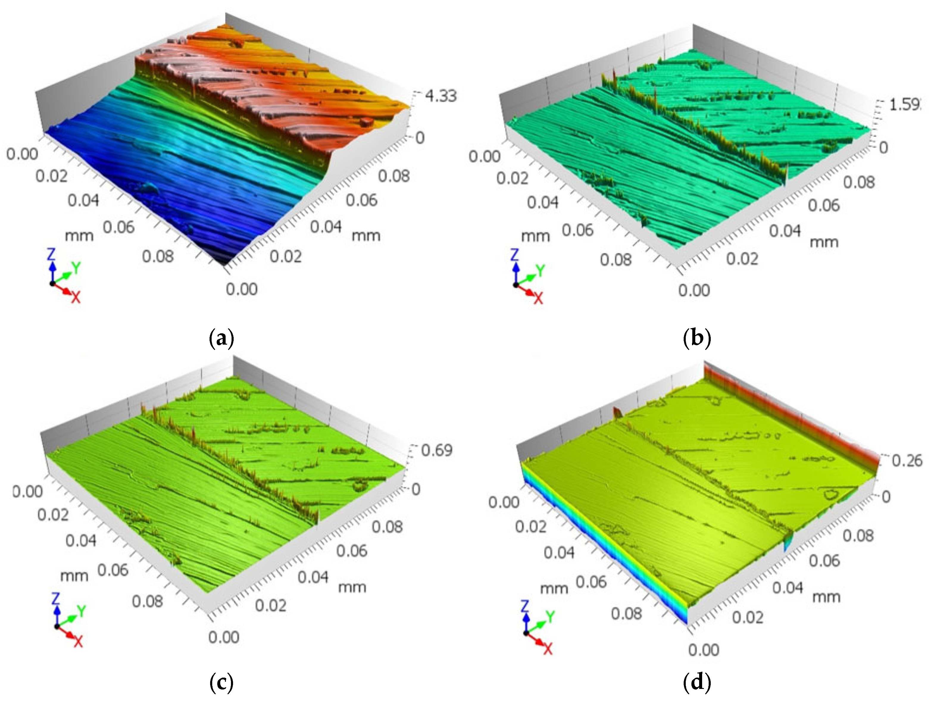
| Sz (μm) | 4.338 | 1.593 | 0.691 | 0.268 |
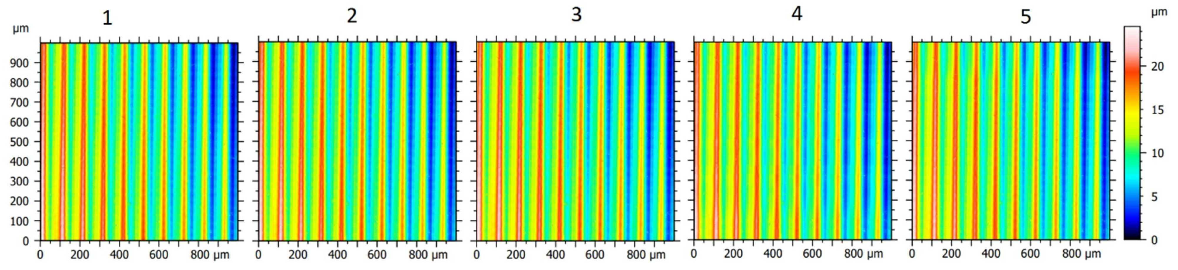
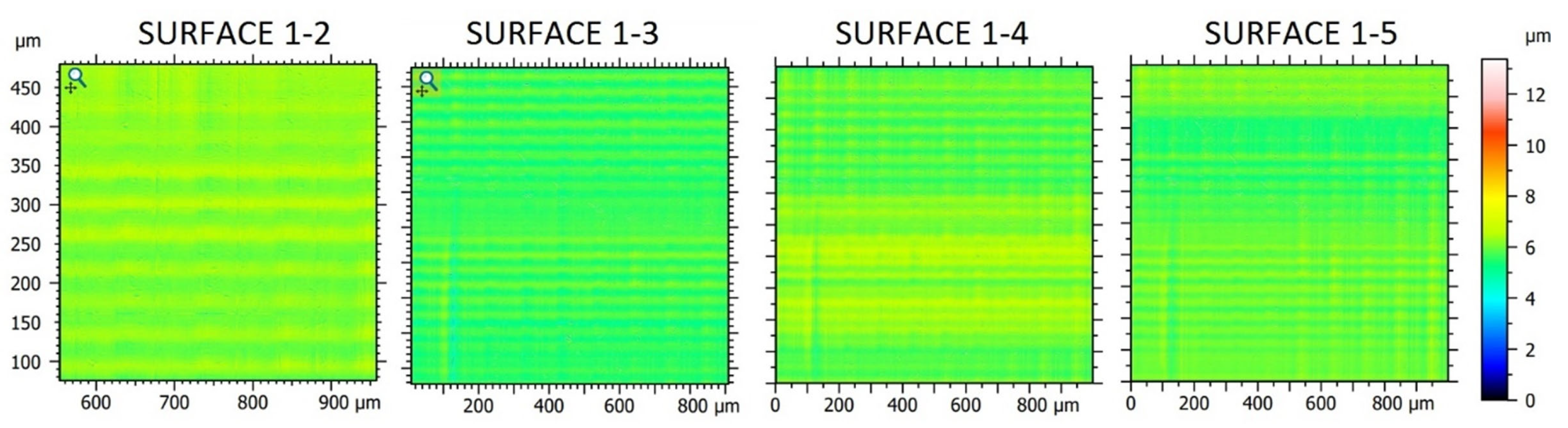
| RS No. | Sq (μm) | (μm) | Noise (RS-MS) 1 (µm) | ||||
|---|---|---|---|---|---|---|---|
| MS No. 1 | MS No. 2 | MS No. 3 | MS No. 4 | MS No. 5 | |||
| 1 | 3.64 | 0.231 | – | 0.260 | 0.237 | 0.207 | 0.221 |
| 2 | 3.74 | 0.196 | 0.260 | – | 0.163 | 0.229 | 0.237 |
| 3 | 3.73 | 0.199 | 0.237 | 0.163 | – | 0.224 | 0.207 |
| 4 | 3.74 | 0.239 | 0.207 | 0.229 | 0.224 | – | 0.221 |
| 5 | 3.76 | 0.231 | 0.221 | 0.237 | 0.207 | 0.221 | – |
| Parameter | Description | Master Value | Master Value with White Noise | Master Value with Brown Noise |
|---|---|---|---|---|
| Sq (μm) | RMS deviation of the surface | 4.9507 | 4.9763 | 4.9967 |
| Sp (μm) | Maximum surface peek height | 7.0000 | 9.3947 | 8.7055 |
| Sv (μm) | Lowest valley of the surface | 7.0000 | 9.3712 | 8.6092 |
| Sz (μm) | Maximum height of topographic surface | 14.0000 | 18.7658 | 17.3147 |
| Sa (μm) | Arithmetic mean deviation | 4.4581 | 4.4695 | 4.4845 |
| St (μm) | Total height of surface | 14.000 | 18.7658 | 17.3147 |
| Parameter | Description | Master Value | Master Value with White Noise | Master Value with Brown Noise |
|---|---|---|---|---|
| Sq (μm) | RMS deviation of the surface | 4.9507 | 4.9503 | 4.9730 |
| Sp (μm) | Maximum surface peek height | 7.0000 | 7.2153 | 7.4219 |
| Sv (μm) | Lowest valley of the surface | 7.0000 | 7.2185 | 7.4115 |
| Sz (μm) | Maximum height of topographic surface | 14.0000 | 14.4338 | 14.8334 |
| Sa (μm) | Arithmetic mean deviation | 4.4581 | 4.4575 | 4.4475 |
| St (μm) | Total height of surface | 14.000 | 14.4338 | 14.8334 |
| Parameter | Description | Raw Master Value | After Wavelet Filtering | After Gaussian Filtering (250 µm) |
|---|---|---|---|---|
| Sq (μm) | RMS deviation of the surface | 3.7874 | 3.7826 | 2.5796 |
| Sp (μm) | Maximum surface peek height | 9.4247 | 9.1543 | 7.3722 |
| Sv (μm) | Lowest valley of the surface | 7.2324 | 6.7996 | 5.8757 |
| Sz (μm) | Maximum height of topographic surface | 16.6571 | 15.9539 | 13.2479 |
| Sa (μm) | Arithmetic mean deviation | 3.1822 | 3.1804 | 2.1088 |
| St (μm) | Total height of surface | 16.6571 | 15.9539 | 13.2479 |
| Parameter | Values after Using High-Pass Gaussian Filter and Wavelet Transform | |||
|---|---|---|---|---|
| Raw Surface | Gaussian λc = 2.5 | Kinsburry 1-Level | UKin (µm) | |
| Sq (μm) | 1.262 | 0.034 | 1.261 | ±0.030 |
| Sa (μm) | 1.183 | 0.015 | 1.182 | ±0.006 |
Disclaimer/Publisher’s Note: The statements, opinions and data contained in all publications are solely those of the individual author(s) and contributor(s) and not of MDPI and/or the editor(s). MDPI and/or the editor(s) disclaim responsibility for any injury to people or property resulting from any ideas, methods, instructions or products referred to in the content. |
© 2024 by the authors. Licensee MDPI, Basel, Switzerland. This article is an open access article distributed under the terms and conditions of the Creative Commons Attribution (CC BY) license (https://creativecommons.org/licenses/by/4.0/).
Share and Cite
Grochała, D.; Grzejda, R.; Parus, A.; Berczyński, S. The Wavelet Transform for Feature Extraction and Surface Roughness Evaluation after Micromachining. Coatings 2024, 14, 210. https://doi.org/10.3390/coatings14020210
Grochała D, Grzejda R, Parus A, Berczyński S. The Wavelet Transform for Feature Extraction and Surface Roughness Evaluation after Micromachining. Coatings. 2024; 14(2):210. https://doi.org/10.3390/coatings14020210
Chicago/Turabian StyleGrochała, Daniel, Rafał Grzejda, Arkadiusz Parus, and Stefan Berczyński. 2024. "The Wavelet Transform for Feature Extraction and Surface Roughness Evaluation after Micromachining" Coatings 14, no. 2: 210. https://doi.org/10.3390/coatings14020210