Abstract
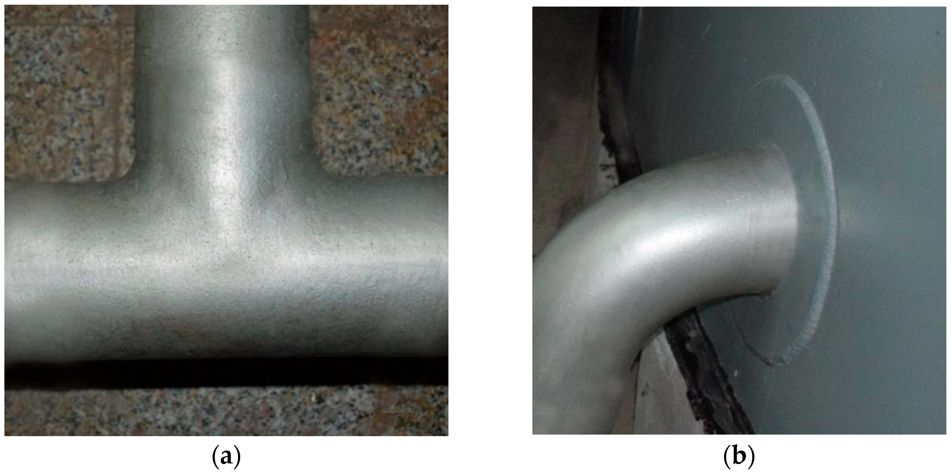
Unidiameter Vertical Interpenetrating Cylindrical Surfaces (UVICS, also called T-pipe surfaces) are a type of typical complex surface that exists in facilities or equipment such as oil storage tanks and industrial pipelines. The shape and surface characteristics of a component undergoing spraying will have a significant impact on the spray flow field and the resulting coating film. In order to optimize the coating effects of complex surfaces, the Euler-Euler approach was utilized to model a spray film formation process that encompasses both a spray flow field model and a wall adhesion model. Subsequently, the influence of the geometric features, geometric dimensions, lateral air pressure of the spray gun, and spraying distance on the coating film characteristics of this kind of surface were systematically investigated. It is determined that the film thickness uniformity could be enhanced by decreasing the dimensions of the workpiece or increasing the lateral air pressure and spraying distance in an appropriate manner when spraying at the location with the most complex geometric features of UVICS. Furthermore, the optimal parameters under varying spraying conditions were identified. The experiments validated the accuracy of the numerical simulation results and demonstrated the feasibility of this simulation model. The study is of significant value in addressing the challenges associated with film formation during spraying on complex surfaces, developing a comprehensive theoretical framework for air spraying, and expanding the scope of applications for automatic spraying technology.
1. Introduction
Industrial metal facilities and equipment are susceptible to corrosion due to environmental influences, which affects product performance and longevity [1,2,3]. For coating and corrosion protection, robotic air spray technology is increasingly being used [4,5]. Air spraying [6] is a relatively common method employed in the field of anti-corrosion engineering as well as an effective method for addressing the limitations of airless spraying [7,8], such as the ease with which the painted film rebounds and its inability to be used for fine spraying. The sprayed coating thickness is evenly distributed, and the surface of the coating film is smooth and precise. In air spraying technology, paint and compressed air are sprayed from orifices, and the paint droplets are atomized under the impact of high-pressure gas, adhering to the surface of the workpiece to form coatings.
In the majority of cases, complex surfaces are sprayed during the spraying process. Spraying on complex surfaces results in a deterioration of the quality of the film due to the specific characteristics of these surfaces. The reason for this is a lack of understanding of the characteristics and mechanisms of film formation on complex surfaces, which makes it difficult to set optimal spraying parameters when spraying. One effective approach to addressing this challenge is to utilize computational fluid dynamics (CFD) to investigate the film formation characteristics of complex surfaces. The air spraying process can be described as a rather complex two-phase flow of gas and liquid. Two-phase flow treatments in CFD can be classified into two categories: the Euler-Lagrange approach [9,10] and the Euler-Euler approach [11,12], based on the different treatments of the two phases. Both approaches consider the gas phase to be a continuous phase, but the former considers the paint phase to be a discrete phase, whereas the latter considers the paint to be a continuous phase. In initial studies, the Euler-Lagrange approach was typically utilized for investigations into the film formation of spraying. In order to gain insight into the characteristics of spray films formed on rectangular groove surfaces [13] and saddle ridge surfaces [14], modeling was conducted to simulate the formation of spray films on different-shaped surfaces. Xie et al. [15] conducted numerical simulations of spraying on a circular surface to examine the influence of air pressure and workpiece geometry on the coating film thickness distribution. Nevertheless, the Euler-Lagrange approach is computationally demanding and requires high cell quality, rendering it unsuitable for the study of engineering problems. In recent years, researchers have also achieved promising results by utilizing the Euler-Euler approach for numerical simulation of film formation characteristics. Chen W. et al. [16] developed static and dynamic spray film formation models for arcuate surfaces and obtained the spray flow field characteristics and film thickness distribution characteristics. Chen S. et al. [17] also carried out a study on the film formation characteristics of V-shape surfaces with different angles.
For model comparison, the same airless spraying film formation numerical simulation based on the Euler-Euler approach and the Euler-Lagrange approach, respectively, investigated by Yang et al. [18,19] revealed that the model based on the Euler-Euler approach only took half the time of the other and achieved the same level of solution accuracy. On the contrary, Yi et al. [20,21] considered it more suitable for modeling the spraying process using the Euler-Lagrange approach owing to the low volume fraction of the droplet phase. Aimed at this academic debate of multiphase flow model selection, Wu et al. [22] present an in-depth analysis of the various two-phase flow modeling methods and their respective advantages and disadvantages in their comprehensive review and conclude that the Euler-Euler approach is more suitable for addressing complex gas-liquid two-phase flow. This approach is capable of accurately simulating the turbulent transport process of liquid droplets in air, providing a detailed understanding of the liquid-phase velocity, concentration distribution, and other crucial aspects. Additionally, the computed shapes of the coating film exhibit enhanced accuracy and a reduced computational volume, making it a highly effective approach. Consequently, the Euler-Euler approach is well suited for studying gas-liquid two-phase flows such as spray flow field motions, jets, and pipe flows in engineering application problems.
Vertical interpenetrating cylindrical surfaces, which are a common type of complex surface in the industry, are formed by two cylindrical surfaces running vertically through, as illustrated in Figure 1. These surfaces can be categorized into two distinct types: unidiameter ones (UVICS, also known as T-pipe surfaces) and non-equal-diameter ones (NVICS, also known as branching pipe surfaces). The complex geometry and surface characteristics of these surfaces result in a lack of uniformity in the coating film during spraying. To date, there is a paucity of literature on the subject of film formation characteristics in the context of spraying on these kinds of surfaces.
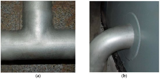
Figure 1.
Engineering application of vertical interpenetrating cylindrical surfaces. (a) UVICS; (b) NVICS.
In this paper, the Euler-Euler approach was utilized, in conjunction with a turbulence model and a wall adhesion model, to investigate the film formation characteristics of UVICS through modeling and numerical simulation. It is expected to reveal the differences in the spraying film formation characteristics resulting from variations in the shape characteristics and the spraying parameters, which can provide references to the research on the film formation of similar-shaped surfaces and their engineering applications.
2. Modeling
2.1. The Air Spraying Process
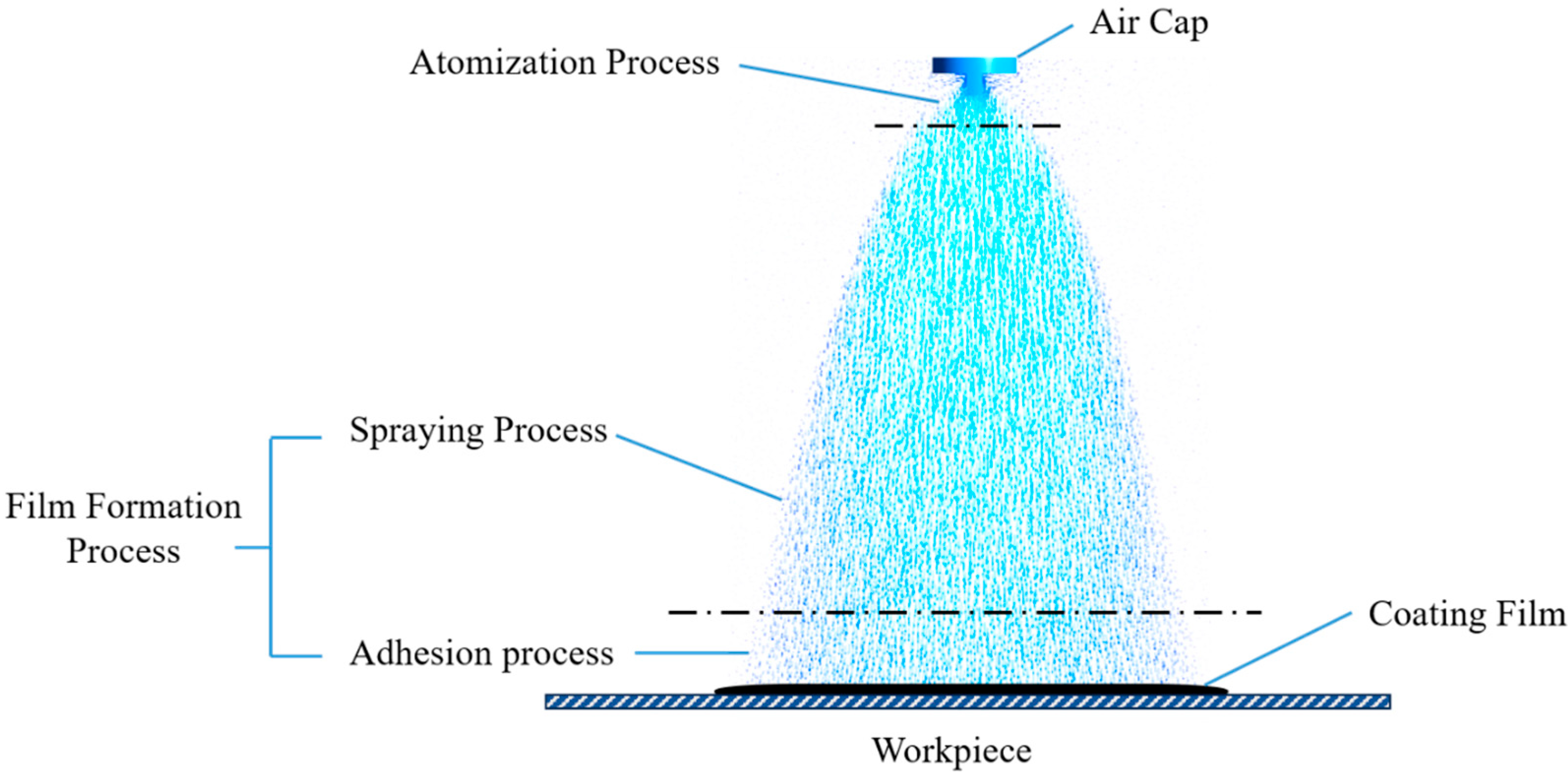
According to the time sequence, air spraying can be divided into an atomization process and a film formation process, as shown in Figure 2. In practical engineering applications, it is more concerned with film thickness and film uniformity in the film formation process, which can be further divided into a spraying process and an adhesion process. Accordingly, the aforementioned two processes are modeled, respectively.
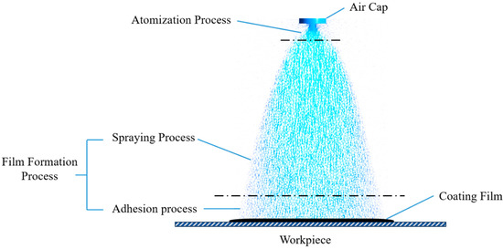
Figure 2.
Air spraying process.
2.2. Spray-Flow Field Model
The phase volume rate of the gas-liquid phase in the control body can be expressed as follows:
where the subscript g denotes the gas phase and the subscript l denotes the liquid phase, and the sum of the gas-liquid phase volume rates is equal to 1 in the spray flow field.
The ambient temperature remains constant throughout the spraying process, and the spray time is relatively brief. Consequently, the heat transfer phenomenon in the two-phase flow can be disregarded, and only the two-phase mass conservation equation and momentum conservation equation can be established. The mass conservation equation is as follows:
where ρq is the density of the q phase and vq is the velocity of the q phase. The momentum conservation equation is as follows:
where p is the pressure between the two phases, g is the gravity τq is the viscous stress in phase q, and Fq is the drag force.
Given that the spraying process is regarded as a continuous two-phase flow, the force between the phases is dominated by the drag force. The paint droplets are regarded as ideal spheres, and the ratio of air density to droplet density is much less than 1. As a result, the flow process between the two phases will transfer momentum, which means that the drag force Fd is more suitable to be calculated using the Schiller and Naumann drag force models. When all subscripts q in Equation (3) are changed to l, which is the equation for the conservation of droplet phase momentum, the drag force of air relative to the liquid phase is as follows:
where is the relaxation time of the droplets, which can be further expressed as follows:
where μ is the molecular viscosity of the fluid, dl is the droplet diameter, CD and Rel are the coefficient of drag force and droplet Reynolds number, respectively, which can be further expressed as follows:
Upon substituting all subscripts “q” in Equation (3) with “l”, the resulting equation becomes a momentum conservation equation for the gas phase. Consequently, the drag force can be expressed as the sum of the reaction forces of the gas phase and the drag force of all droplet phases, as is written below:
In the modeling of turbulence, the standard k-ε turbulence model is selected, which belongs to the Reynolds-averaged simulation (RANS) method. This model is capable of meeting the computational accuracy requirements for air spraying. The vortex-viscous model is utilized for the processing of the Reynolds stress term in the model, thereby enhancing the computational efficiency. The relationship between the mean velocity gradient and the Reynolds stress in the vortex-viscous model is as follows:
where the variables , , and k represent the turbulent viscosity, the time-averaged velocity, and the turbulent kinetic energy, respectively. The standard k-ε turbulence model comprises equations for turbulent kinetic energy and turbulent energy dissipation rate. Among these, the turbulent dissipation rate is expressed as:
where the turbulent viscosity is a function of k and ε. It can be expressed as follows:
where is an empirical constant, here taken to be 0.09. In the standard k-ε model, the transport equation containing k and ε is as follows:
where the generation term for turbulent energy k is denoted by , is the generation term for turbulent energy k due to buoyancy, is the pulsation expansion in the turbulence. , and are empirical constants, while the Prandtl numbers, and , correspond to k and ε, respectively. Finally, and are the user-defined source terms.
2.3. Near-Wall Model
The standard k-ε turbulence model is only applicable to fully developed turbulence. In the near-wall region, however, the reduction in the Reynolds number makes the turbulence incompletely developed. Consequently, the standard wall function method is utilized to describe the near-wall flow. When the dimensionless distance , the spray has fully developed turbulence. At this point, it can be assumed that the expressions for the dimensionless velocity , the dimensionless distance and the wall shear stress are as follows:
By contrast, when , the spray turns into an incompletely developed laminar flow, situated within the viscous bottom region. The dimensionless velocity then conforms to the laminar strain relation, as expressed by the following equation:
where is the Karman constant and E denotes an empirical constant, denotes the time-averaged velocity of the node, yp represents the distance from the node to the wall, and kp is the turbulent kinetic energy of the node, which is expressed in the wall region as follows:
where n denotes the coordinates perpendicular to the wall.
At this point in time, both the turbulent dissipation rate (ε) and the turbulent kinetic energy production term (Gk) are modified. They are both equal at the nodes in the wall region, as expressed by the following equation:
2.4. Eulerian Wall Film Model
Upon collision with the wall, the paint droplets adhere to the wall, forming a coating film. This process results in a change in the droplets’ mass and momentum, which are then used as the source term and added to the wall liquid film control equation set to establish the touch wall adhesion model. The expression for the mass source term of the liquid phase, , is as follows:
where denotes the normal velocity of the liquid phase with respect to the wall, denotes the volume fraction of the liquid phase, denotes the density of the liquid phase, and A denotes the area of the wall. The expression for the momentum source term of the liquid phase, , is as follows:
where is the velocity vector of the liquid phase.
The thickness of the liquid film can be determined by establishing the mass and momentum conservation equations for the liquid film and then solving the resulting equations. The mass conservation equation, which is established by adding the mass source term of the liquid phase to the system of equations, is as follows:
where h, and are the thickness, the density, and the average velocity of the liquid film, respectively. Similarly, by adding the momentum source term for the liquid phase to the equations, the momentum conservation equation established is as follows:
The above equation comprises two terms on the left side, representing the transient change of the liquid phase and convective transport, respectively. The right side of the equation represents the combined effect of the flow field pressure, the liquid film surface tension, and the gravity component on the vertical wall, the effect of gravity on the liquid film in the parallel direction, the effect of viscous shear at the gas-liquid interface, the viscous force of the liquid film on the wall, and the formation of the momentum source term in the liquid film, respectively.
Once the model has been established, it is then discretized in space by the Finite Volume Method (FVM), discretized in time by the fully implicit method, and solved by the PC-SIMPLE algorithm. This process enables the acquisition of data pertaining to the flow field and the coating film of the spray film-forming process.
3. Simulation and Experimental Details
3.1. Geometric Model and Fluid Regions
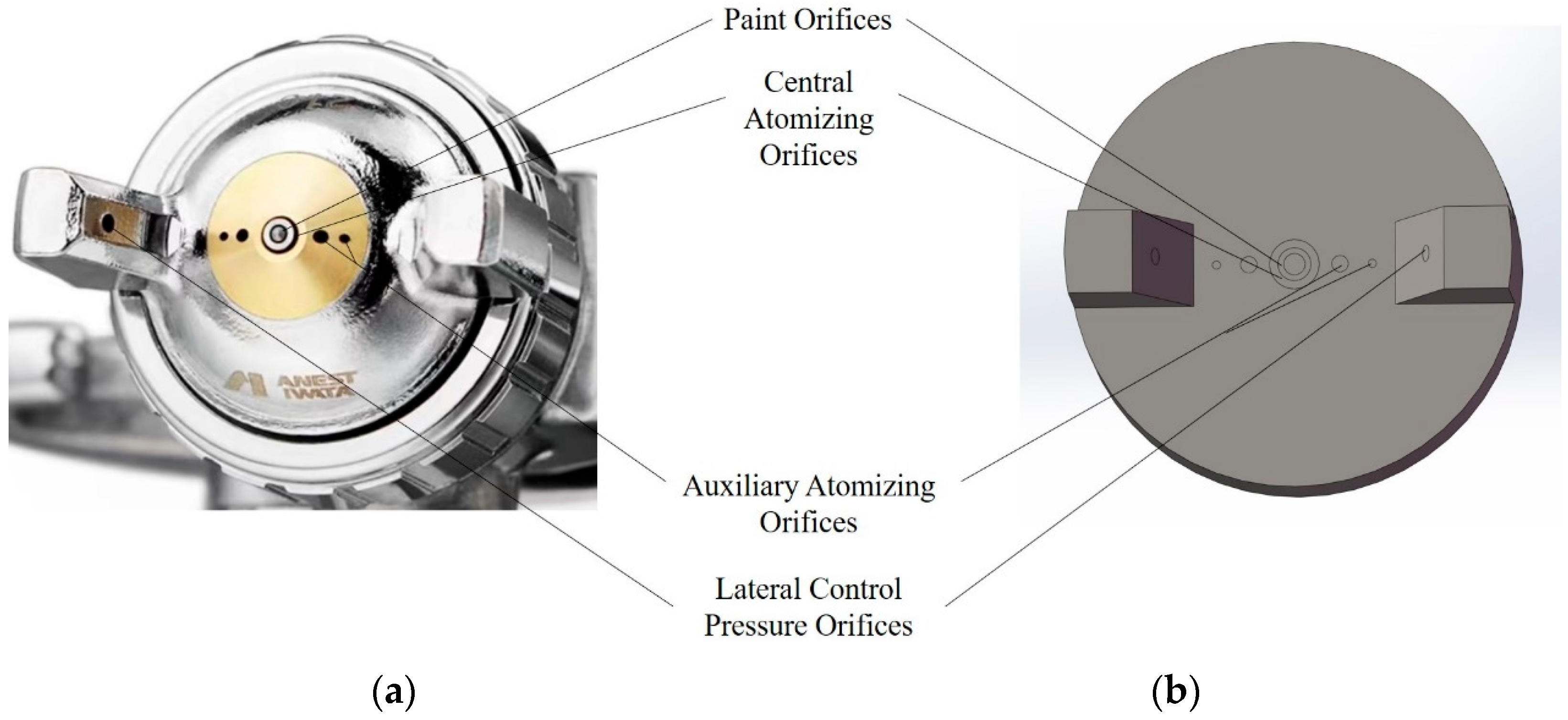
The geometric structure of the air cap of the W-71C-21S air spray gun (ANEST IWATA Co., LTD, Yokohama, Japan) is chosen as a model basis. The non-critical geometric structure is then simplified, and the air cap of the spray gun and the geometric model of the air cap are presented in Figure 3.

Figure 3.
The air cap of the spray gun. (a) Actual air cap; (b) Air cap model.
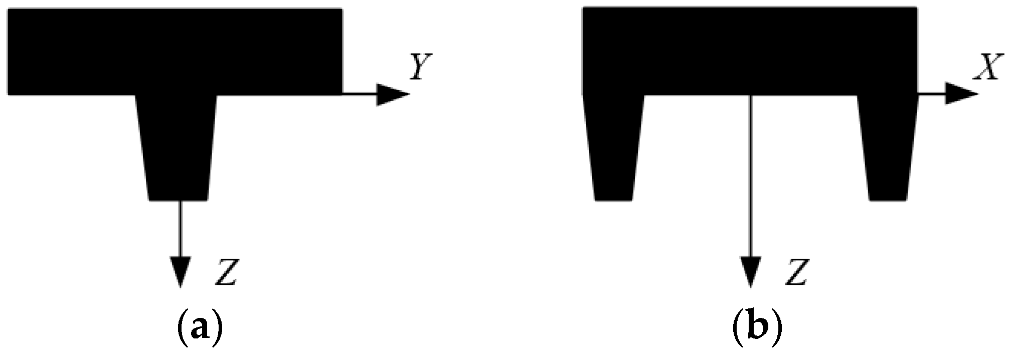
Take the air cap of the spray gun as a reference to establish a 3D right-angle coordinate system, as illustrated in Figure 4. The origin of the coordinate system is at the center of the paint orifice; the X-axis coincides with the line of the center of the four auxiliary atomizing orifices; the Y-axis is set in the plane of the paint orifice and the central atomizing orifice and is perpendicular to the X-axis as well; and the Z-axis is directly opposite to the direction of the paint orifice and is perpendicular to the XY plane.
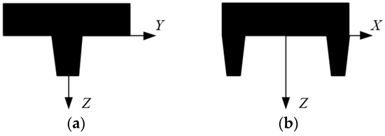
Figure 4.
Coordinate system of the spray flow field. (a) YZ; (b) XZ.
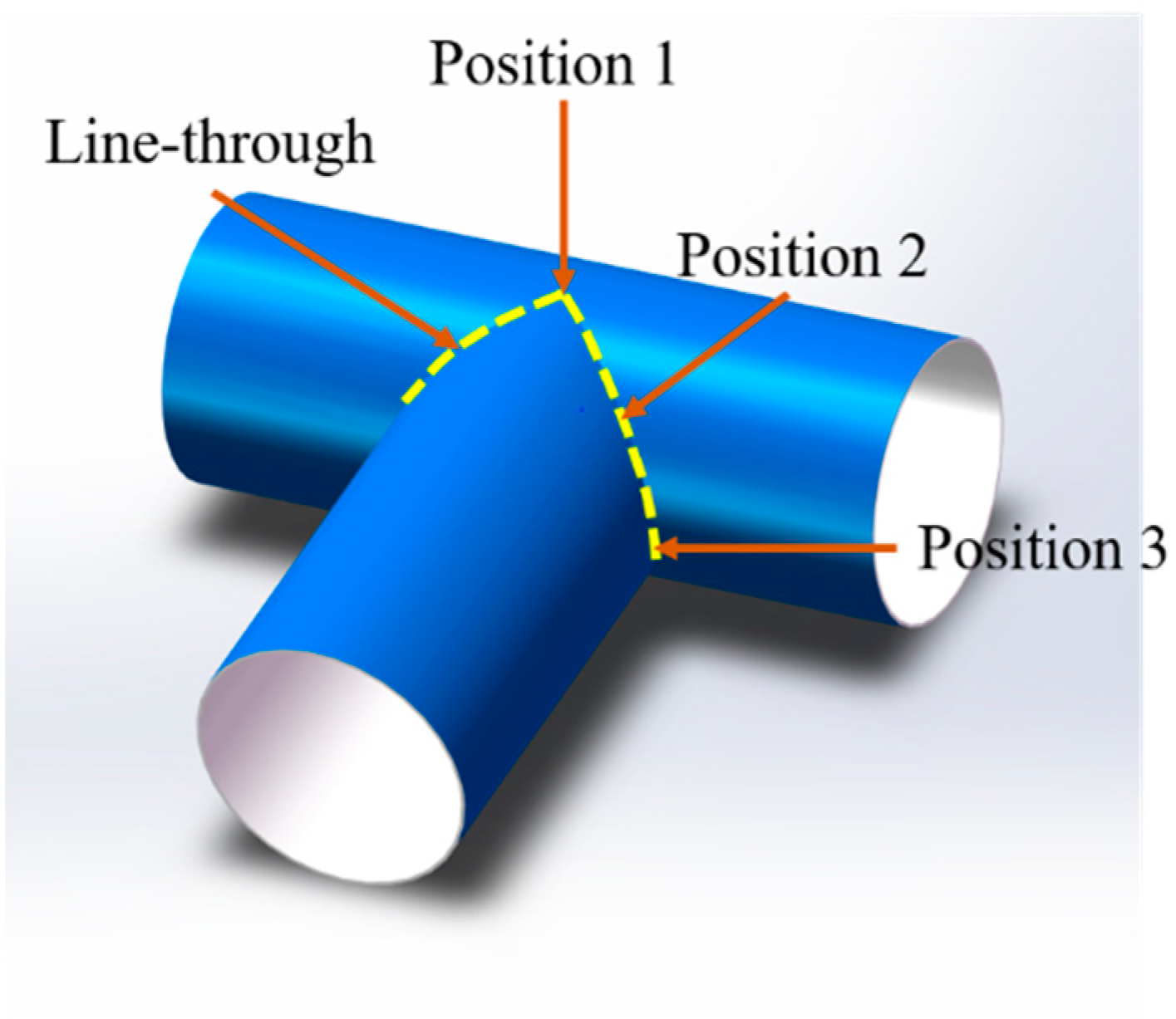
Aiming at the geometrical characteristics of the three typical positions of UVICS, three representative positions, designated as Position 1, Position 2, and Position 3, as illustrated in Figure 5, have been selected for the purpose of conducting a numerical simulation study of air spraying. Position 1 is the intersection of the line-through of the two cylindrical surfaces, while Position 2 and 3 are the 45° and 90° oblique positions along the line-through. (For the sake of simplicity, the simulations or experiments of spraying on three different positions will be referred to as “#1”, “#2”, and “#3” in the following text). Furthermore, the fluid domain is constructed according to a spraying distance of 200 mm and an outer diameter of the cylinder of 150 mm. Meanwhile, for verification and comparison, a plane with a size of 200 mm × 200 mm is selected for numerical simulation of film formation, as shown in Figure 6 (again, it will be referred to as “#0”).

Figure 5.
3D geometric model of UVICS.
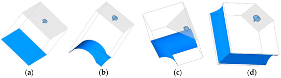
Figure 6.
Fluid regions of the plane and UVICS. (a) #0; (b) #1; (c) #2; (d) #3.
3.2. Meshing and Mesh Independence Validation
The polyhedra is selected for meshing, and #0 is selected for showing the mesh independence validation process. The validated mesh size, quantity, and quality are presented in Table 1, and the corresponding trends in mesh properties are illustrated in Figure 7a. It can be observed that the number of cell numbers drawn gradually increases, the average mesh quality gradually increases, and the average skewness gradually decreases as the maximum mesh length gradually decreases. In addition, the calculated axial gas phase velocities in the flow field with different mesh sizes were selected as a test basis, as shown in Figure 7b. It was found that the key features of the spray flow field could be accurately captured with a maximum mesh length of 0.002~0.005 m. In order to save computational cost and maintain good computational accuracy as a wall, the maximum mesh length of 0.003 m was selected for subsequent simulation calculations.

Table 1.
Mesh parameters.
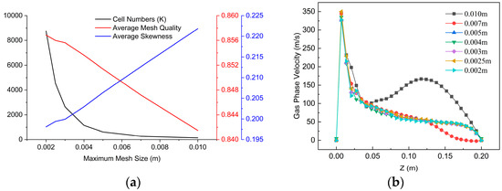
Figure 7.
Validation of mesh independence. (a) Mesh parameters; (b) Gas phase velocity along the Z-axis.
3.3. Set-Up and Boundary Conditions
Set the air to the primary phase and the paint to the secondary phase. Ambient pressure and air density were kept at the system’s default values. Measurements of the physical parameters of the coatings revealed a density of 1.21 × 10³ kg/m3, a viscosity of 0.097 kg/(m∙s), and a surface tension of 2.87 × 10⁻² N/m. In addition, the paint orifice is set as a mass flow inlet with a mass flow rate of 2.8 × 10⁻³ kg/s, a turbulence intensity of 5%, and a hydrodynamic diameter of 1.3mm. The central atomization orifice, the auxiliary atomization orifices, and the lateral pressure orifices are all set as pressure inlets with a pressure of 0.29 MPa and a turbulence intensity of 5%. The hydrodynamic diameters of the central atomization orifice, the auxiliary atomization orifices, and the lateral pressure orifices are 1 mm, 1 mm, and 0.5 mm, respectively. Each time step size is 1 × 10⁻⁴ s, and the total spray duration is 0.5 s.
3.4. Experimental Details
In order to verify the accuracy and precision of the numerical simulation results, spraying experiments need to be conducted in accordance with the same simulation parameters. The workpiece to be sprayed was welded from two unidiameter GB-Q235 steel pipes, and the weld seam was subsequently polished smooth afterward. The spraying experiments were carried out in a spraying chamber. Prior to the spraying, the air compressor (Luodi electromechanical Technology Co., LTD., Quzhou, China) was assembled with the air spray gun, which was subsequently mounted on a homemade robotic arm. When completing the spraying, the workpieces were left for three days to allow the coating film to dry naturally. The Smart Sensor AR932 Coating Thickness Gauge (Wanchuang Electronic Products Co., Ltd., Dongguan, China) is utilized to measure the thickness of coating films on workpieces following a period of standing and drying. When measuring, record the coordinate value and coating film thickness at 10 mm intervals. It is also necessary to repeat the measurement three times for each point. The arithmetic average of the coating film thickness at the point was taken as the final thickness.
4. Results and Discussion
4.1. Flow Field Characteristics
4.1.1. Longitudinal Flow Field Characteristics
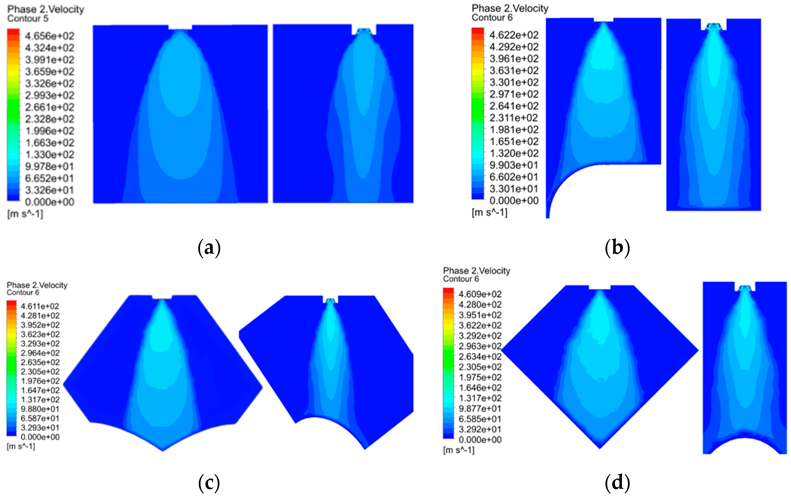
The spray flow field characteristics are described in terms of longitudinal velocity contours for the four spraying conditions, as depicted in Figure 8, with the YZ cross section on the left side and the XZ on the right of each figure. It can be observed that, under the four spraying conditions, the spray flow fields are expanded in the YZ plane and compressed in the XZ plane due to the airflow from the lateral pressure orifices. When the liquid-phase flow field is situated at a greater distance from the wall, the shape of the flow field in the four conditions shows similarity. Conversely, when the liquid-phase flow field is in closer proximity to the wall, the surface geometric characteristics of the four wall surfaces exert a great amount of expansion or compression on the flow field shapes. To illustrate, take the liquid-phase flow field of #3, for instance. In the YZ section, the flow field produces a significant compression due to the 90° cylindrical surface angle included on both sides, resulting in a smaller flow field range than others. In the XZ section, the liquid-phase flow field continues to develop along the wall after contacting the wall, resulting in a larger flow field range than the other three.
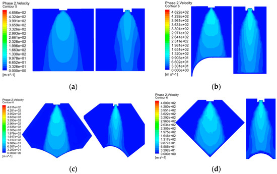
Figure 8.
Longitudinal shapes of liquid flow fields. (a) #0; (b) #1; (c) #2; (d) #3.
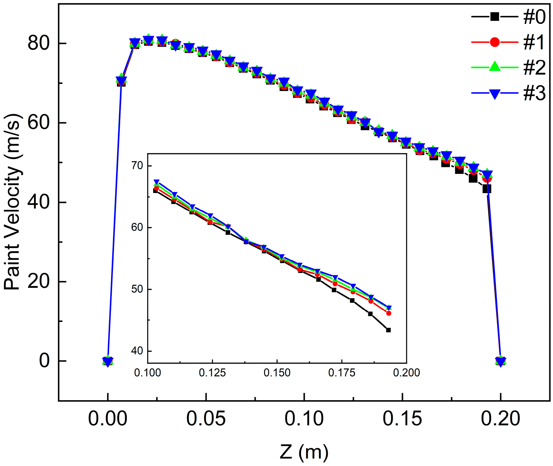
The longitudinal development of paint droplets in the spray flow field is reflected by analyzing the Z-axis paint velocity distributions for different spray cases, as shown in Figure 9. It can be observed that, following the injection of paint via the spray nozzle, the high-pressure airflow and the low velocity of the paint between the momentum transfers occur violently, the paint speed is rapidly accelerated to about 80 m/s, and the paint is rapidly atomized by the impact into fine liquid droplets. Subsequently, the propagation of the liquid phase is impeded by the gas phase, resulting in the dissipation of its kinetic energy. This process results in a gradual reduction in velocity from 80 m/s to 45 m/s. Upon collision with the wall, the droplet adheres, thereby impeding the propagation of the liquid phase. This results in a rapid decrease in velocity, reaching a value of 0 m/s. The inset in the figure illustrates the liquid-phase velocity curves when the Z-axis coordinate range is further narrowed to 0.1~0.2 m. It can be observed that the liquid-phase velocity of #0 is lower than the other three, likely due to the planar feature exerting a stronger hindering effect on the longitudinal spray flow field when the flow field is close to the wall. This results in a faster decay of the liquid-phase velocity, and different locations of the other three all have a certain extension effect on the development of the flow field. In other words, the droplets exhibit lower normal velocities in the near-wall regions of #1, #2, and #3, which makes them less of an impediment to the longitudinal spray flow field.
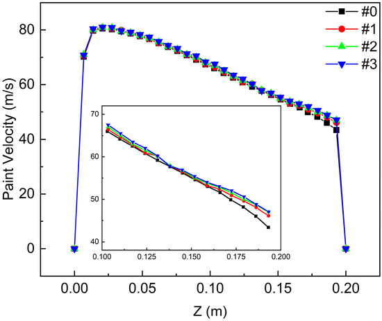
Figure 9.
Paint velocity distribution curves along the Z-axis.
4.1.2. Near-Wall Flow Field Characteristics
As previously stated, the characteristics of the near-wall flow field are significantly influenced by the shape and surface characteristics of the workpiece. Therefore, the XY plane, situated at a vertical distance of 180 mm from the nozzle, is intercepted. The near-wall transverse spray flow field distribution is depicted in Figure 10. The left and right directions in the contours correspond to the X-axis direction, while the top and bottom correspond to the Y-axis direction. The figure illustrates that the morphology of the flow fields of #0 and #1 is relatively similar, exhibiting elliptical distributions. This is due to the lower influence of the near-wall region on the development of the flow field. The extrusion action of the wall relative to the spray flow field results in deformation of the flow field, with notable differences in the shape of the near-wall transverse spray flow field in #2 and #3. The distribution of the former is shell-shaped, while that of the latter is dumbbell-shaped. It is evident that the spray velocity is at its maximum in the center area of the spray cone and decays uniformly along the radial direction.
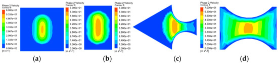
Figure 10.
Velocity contours in a near-wall flow field. (a) #0; (b) #1; (c) #2; (d) #3.
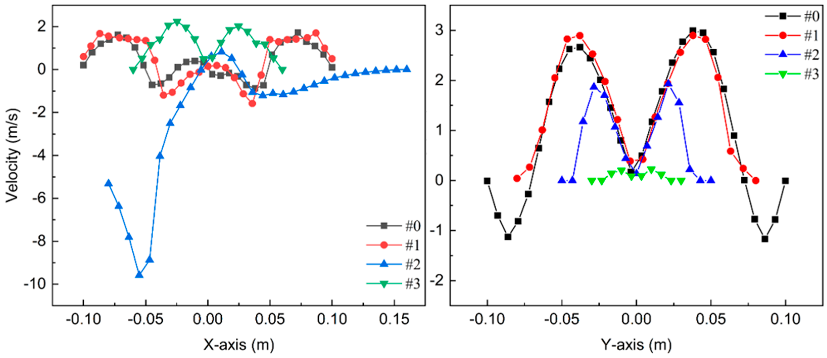
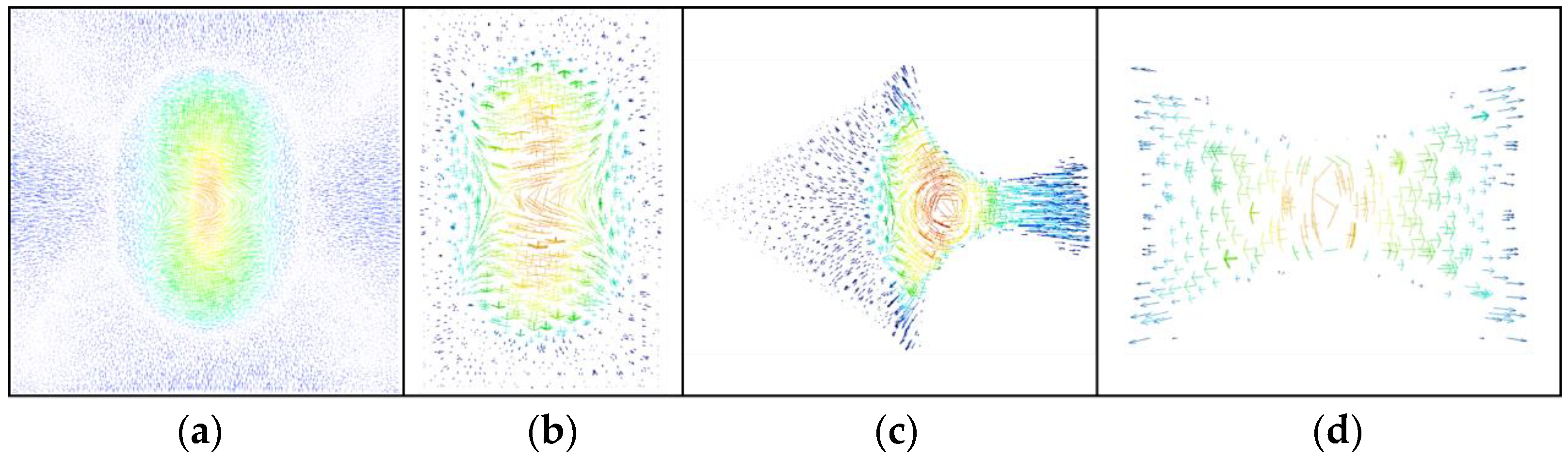
In order to gain insight into the velocity distribution characteristics of paint within the near-wall region, a velocity distribution curve is plotted along the X-axis and Y-axis, respectively, as illustrated in Figure 11. Meanwhile, the near-wall velocity vectors for the four work conditions are shown in Figure 12. It can be observed from Figure 11 and Figure 12. that, in the X-axis direction, the spray velocity distributions of #0 and #1 are similar and symmetrically distributed. However, due to the generation of a vortex near the origin, some of the velocities become negative, indicating the generation of backflow. In comparison to the other three, #2 exhibits a complex and asymmetric shape and surface features. The spray velocity distribution is notably different, exhibiting a substantial increase in spray velocity to −10 m/s in the negative direction, followed by a gradual decrease. This gradual decrease is observed thereafter. This is due to a smaller flow field space in the negative direction, which limits the longitudinal development of droplets and promotes transverse development. Consequently, the spray velocity displays significant variations. The spray velocity distribution of #3 is symmetrical, with the velocity increasing to a maximum value of 2 m/s in both positive and negative directions. Thereafter, the velocity gradually decays to 0 m/s owing to the momentum transfer between the gas and liquid phases. In the Y-axis direction, the spray velocities for all four conditions initially increase and subsequently decrease to zero in both positive and negative directions. However, the distribution ranges and values differ depending on the working conditions. The near-wall spray velocity distribution ranges and values for #2 and #3 are significantly smaller than those of the remaining two, which can be attributed to the fact that the velocity development in the Y-axis direction is hindered by the wall.
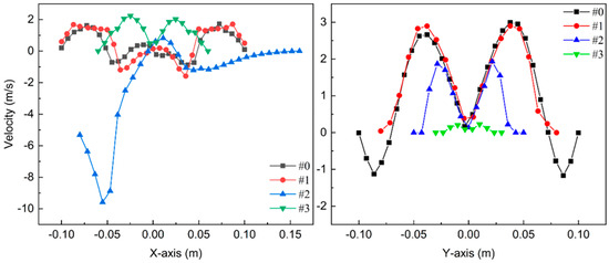
Figure 11.
Velocity distribution curves in a near-wall flow field.
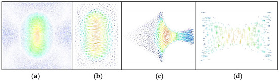
Figure 12.
Velocity vectors in near-wall flow field. (a) #0; (b) #1; (c) #2; (d) #3.
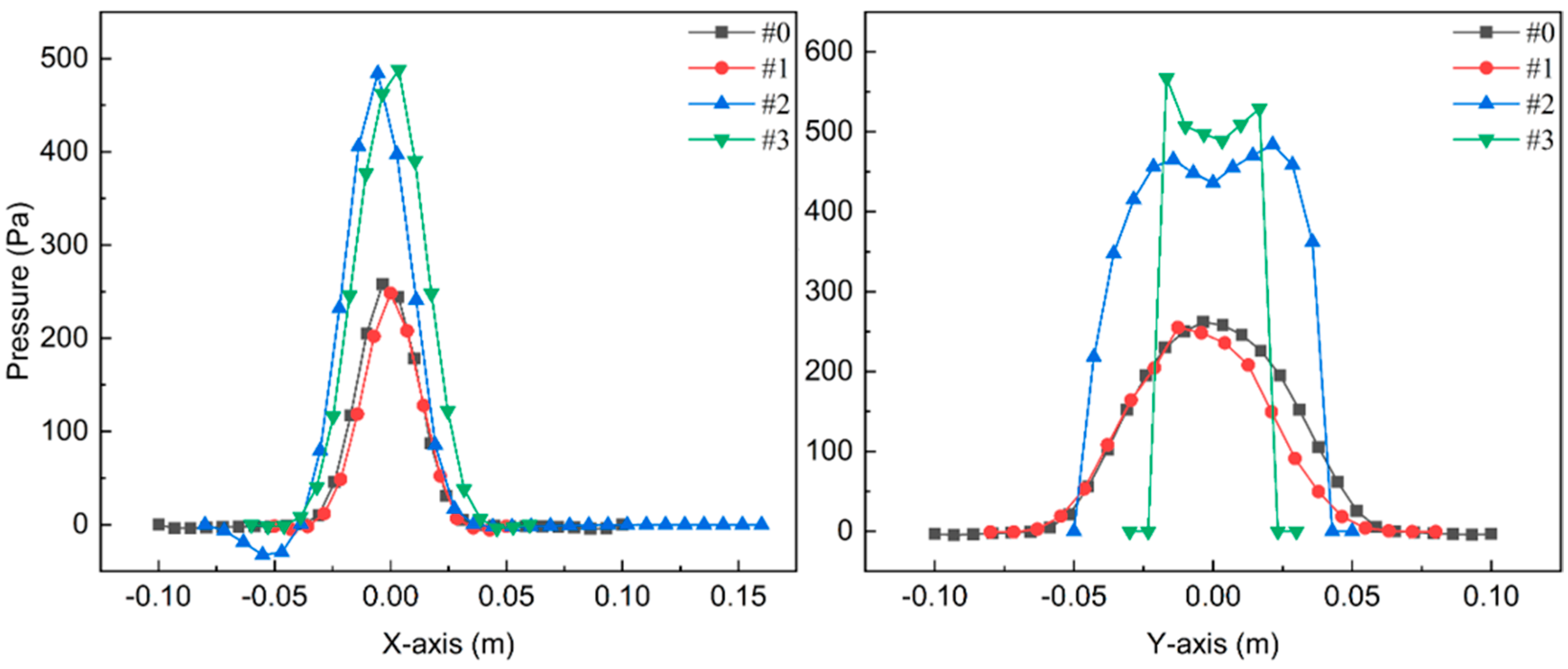
The pressure contours in the near-wall flow field are shown in Figure 13. The pressure in the near-wall flow fields of #0 and #1 reaches its maximum at the center of the spray cone and decays outward in an elliptical ring shape. The pressure outside the spray cone decreases to zero rapidly. By contrast, the pressure in the near-wall flow fields of #2 and #3 reaches its maximum near the wall surface and is distributed in a band-like attenuation pattern. The distribution curves of the near-wall flow field pressure along the X-axis and Y-axis are presented in Figure 14. In the X-axis direction, the pressure curves under the four spraying states exhibit a sharp decline from the origin to zero on both sides, with a pressure distribution ranging from −0.05 m to 0.05 m within the interval. Furthermore, the pressure peaks are observed to be concentrated in the vicinity of the origin. The pressure peaks of #2 and #3 reach 480~490 Pa, which are higher than the pressure peaks of #0 and #1 at 250~260 Pa. In the Y-axis direction, the pressures of #0 and #1 decrease symmetrically on both sides, with a peak pressure of 250 to 260 Pa. In contrast, the pressures of #2 and #3 initially increase and then decrease rapidly from the origin to both sides, with peak pressures of 490 Pa and 560 Pa, respectively. The discrepancy in the pressure peaks can be attributed to the wall surfaces of #2 and #3 in the near-wall region, which act as a direct obstruction to the flow field. This results in a buildup of pressure, in contrast to #0 and #1.
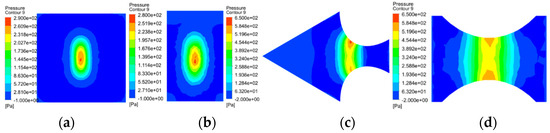
Figure 13.
Pressure contours in a near-wall flow field. (a) #0; (b) #1; (c) #2; (d) #3.
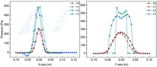
Figure 14.
Pressure distribution curves in a near-wall flow field.
4.2. Influence of Spraying Parameters on Film Characteristics
The shape and surface characteristics of the workpiece exert a significant influence on the flow field near the wall, which in turn affects the coating film effect. Consequently, the subsequent analysis will examine the influence of spraying parameters, including geometric characteristics, dimensions, lateral air pressure, and spraying distance, on the coating film characteristics and the mechanisms of their effects.
4.2.1. Geometric Features
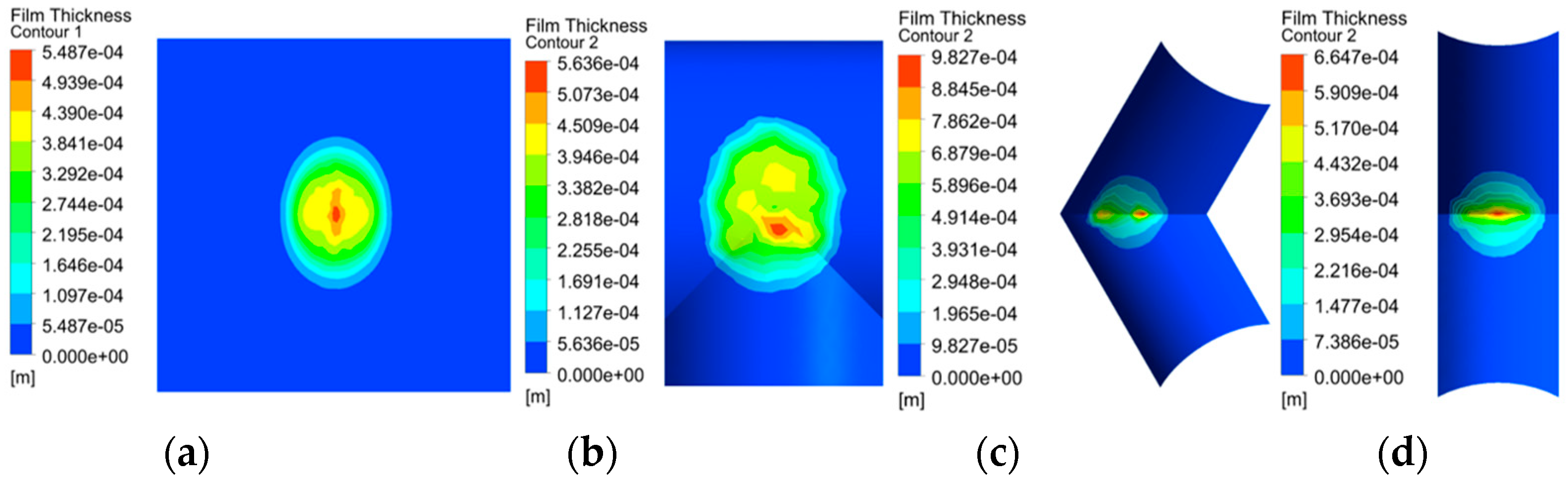
The shape of the coating film contours obtained by numerical simulation for spraying #0 to #3 is illustrated in Figure 15. The left and right directions in the contours correspond to the X-axis direction, while the top and bottom correspond to the Y-axis direction. The film shape of #0 is a typical ellipse obtained by air spraying, with the maximum of the film thickness located at the center. The film shape of #1 is an ellipse with irregular edges. This is due to the raised structure of cylindrical surfaces on the upper and lower sides, which interfere with the motion state of the paint droplets at the edge of the spray cone. The maximum film thickness is near the intersection of the line-through. The film shapes of #2 and #3 can be regarded as two semi-ellipses spliced together. However, the film thickness of #2 exhibits a bimodal distribution along the X-axis direction, with the peak of the film thickness of #3 situated at the center of the film.
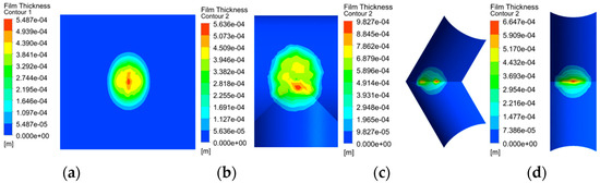
Figure 15.
Film thickness contours of varying geometric features. (a) #0; (b) #1; (c) #2; (d) #3.
The uniformity of the coating film is a crucial parameter for evaluating the quality of the coating film. In order to investigate the uniformity of the coating film thickness in depth and accurately, the film thickness data of the film-forming surface is sampled, and then the Relative Standard Deviation (RSD) [23] of the film thickness is calculated (the data below 10 μm is discarded automatically). The larger the RSD, the more discrete the data distribution; in other words, a smaller RSD means better film thickness uniformity. RSD is expressed as follows:
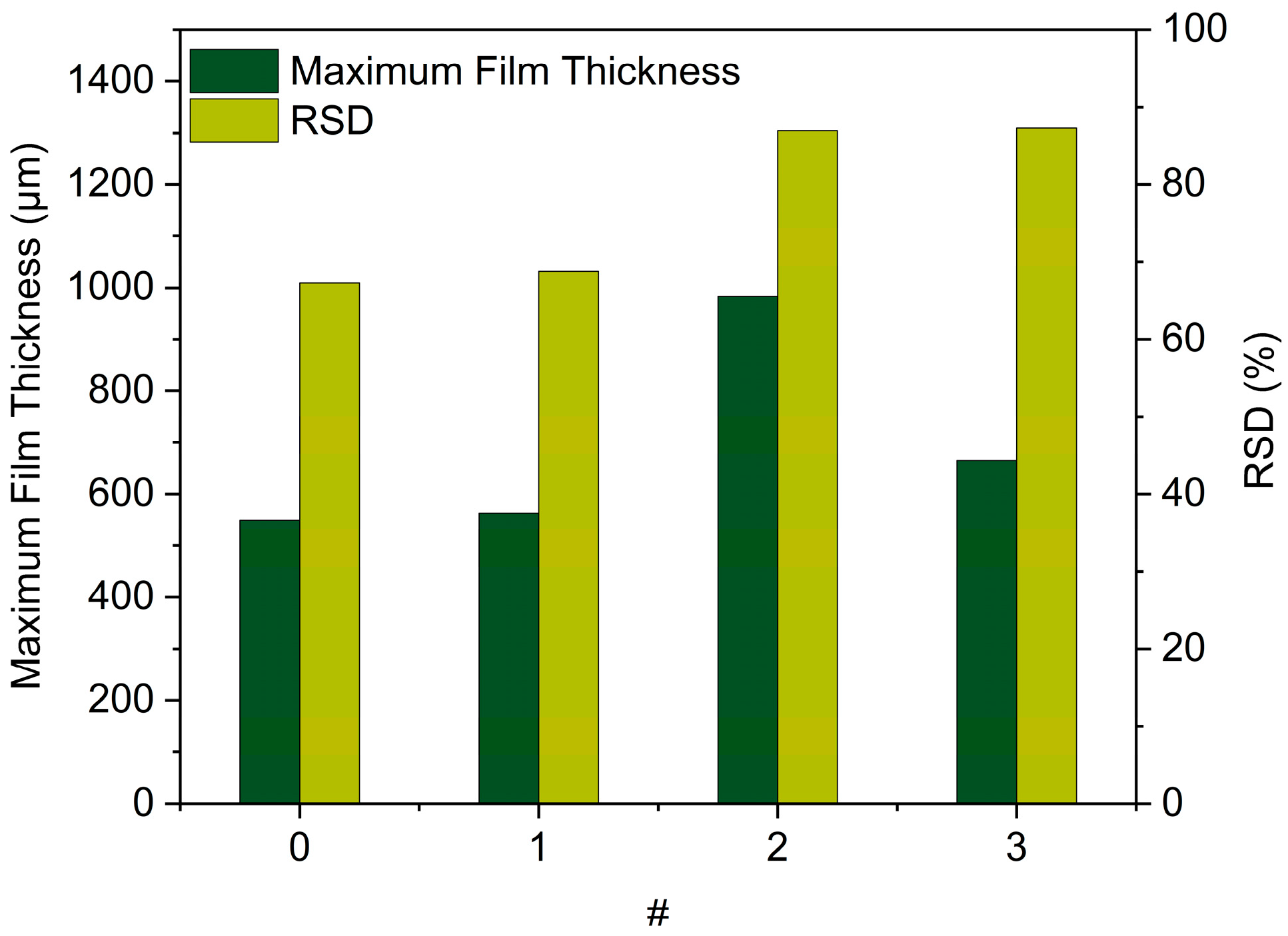
where is the average value of the data. The histograms of maximum film thickness and RSD for the four spraying states are presented in Figure 16. As the most common spraying condition, #0 exhibits an RSD value of 67.29%, which is the lowest of the four surfaces. In contrast, #1 exhibits a slightly higher RSD value of 74.79%, and the RSD values for #2 and #3 are 86.97% and 87.31%, respectively, thereby suggesting that the thickness uniformity of #1 is superior when spraying on UVICS. The film thickness peaks of the four spraying states are 548.7 μm, 563.6 μm, 982.7 μm, and 664.7 μm, respectively.

Figure 16.
Maximum film thickness and RSD of varying geometric features.
4.2.2. Geometric Dimensions
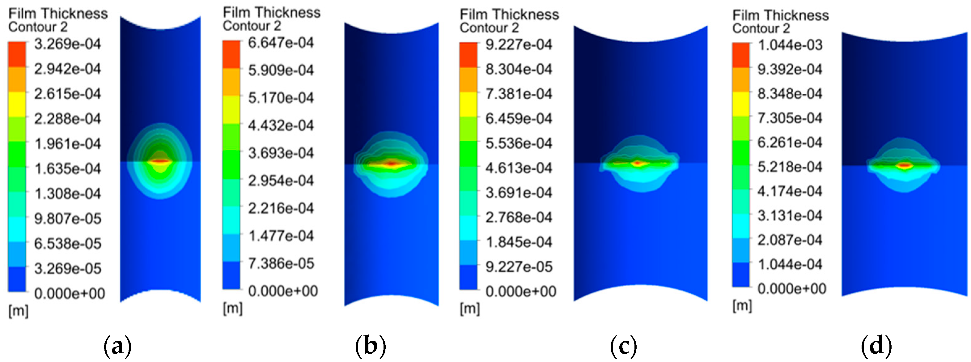
Among the four spraying conditions, the shape and surface characteristics of #3 are the most distinctive and exert the greatest influence on the coating film characteristics. Therefore, #3 is selected for investigation into the influence of geometric dimension, lateral pressure, and spraying distance on the coating film characteristics when spraying on #3. For diameters of the cylindrical tube below 100 mm, plating or brushing for painting is a more suitable method than spraying in industrial applications. Consequently, the cylindrical outer diameters of 100 mm, 150 mm, 200 mm, and 250 mm are selected and named as D100, D150, D200, and D250, respectively. The film thickness contours obtained by numerical simulation are shown in Figure 17. It can be observed that the maximum value of the coating film thickness when spraying all four diameters is at the origin. The length (along the Y-axis) and width (along the X-axis) of the coating film can be obtained by utilizing the differential method to expand the data along the irregular curve into a straight-line arrangement. In the X-axis direction, the coating widths are 120 mm, 122 mm, 146 mm, and 143 mm, respectively. It is notable that the coating widths of D200 and D250 are significantly larger than those of D100 and D150. This phenomenon can be attributed to the decreasing curvature of the line-through as the diameter of the UVICS increases. Namely, the surface geometrical features along the X-axis become increasingly similar to the plane. In the Y-axis direction, the length of the coated film decreases monotonically with the increase of the outer diameter of UVICS to 165 mm, 153 mm, 146 mm, and 143 mm, respectively. Overall, the shape of the coating film becomes flatter as the outer diameter increases. The histograms of maximum film thickness and RSD variation of the four coating films are shown in Figure 18. The film thickness maxima are 326.9 μm, 664.7 μm, 922.7 μm, and 1044 μm, respectively, with respective RSDs of 71.37%, 87.31%, 89.04%, and 90.18%. The film thickness maxima exhibit a trend of fast growth followed by slow growth. It can be observed that, under the condition that other spraying parameters remain unchanged, the UVICS with a diameter of 100 mm has an optimal coating effect when spraying.

Figure 17.
Film thickness contours of varying geometric dimensions. (a) D100; (b) D150; (c) D200; (d) D250.
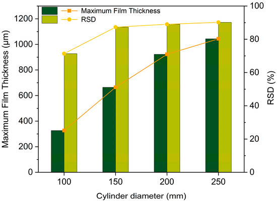
Figure 18.
Maximum film thickness and RSD of varying geometric dimensions.
4.2.3. Lateral Pressure
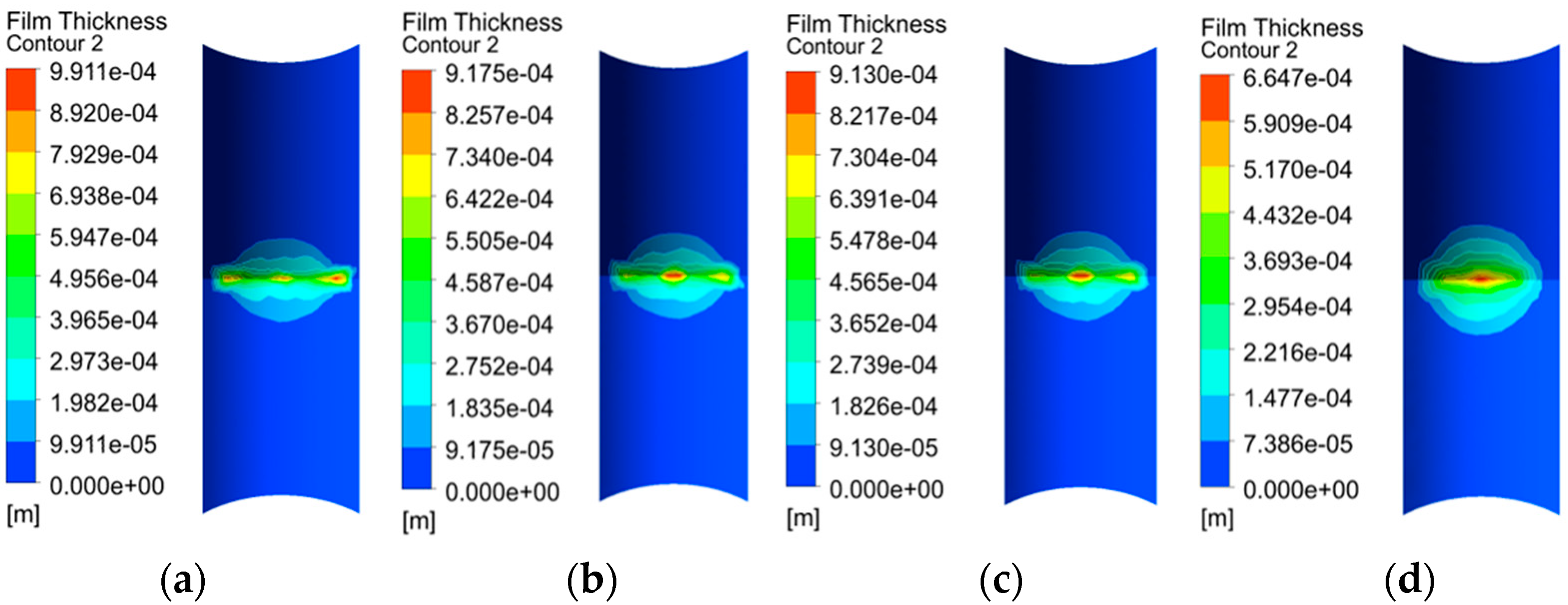
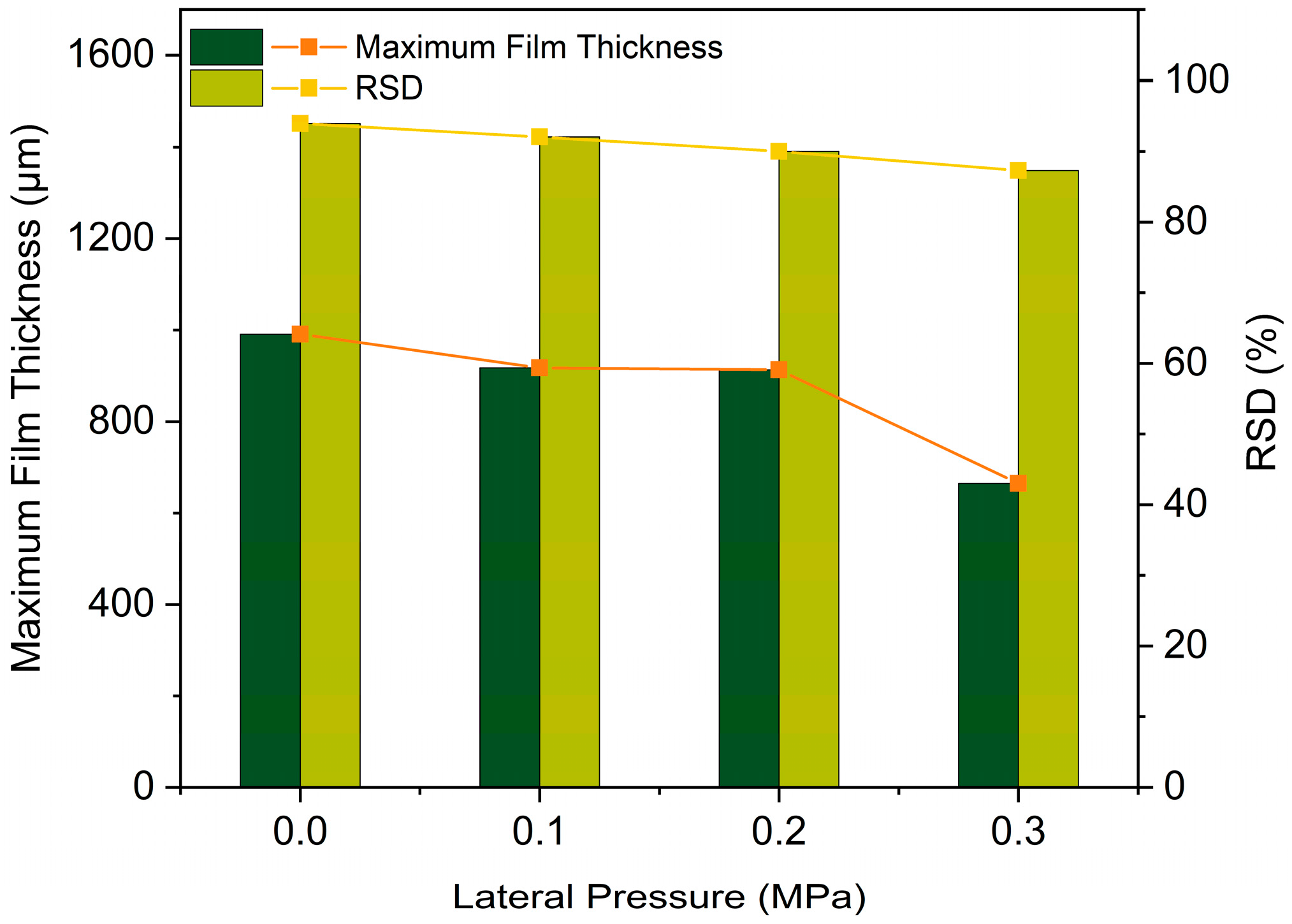
In order to obtain a high-quality coating film when spraying on different-sized workpieces, it is possible to adjust the lateral pressure of the spray gun. The shaping effect of compressed air on the spray flow field enables the aspect ratio of the coating film to be altered, thereby facilitating the control of the quality of the coating film. It is noteworthy that the predominant method of air spraying in the present era is the High Volume Low Pressure (HVLP) method [24]. This is due to the fact that its stable spraying amplitude enables effective improvement of transfer efficiency and reduction of overspray. Consequently, the lateral pressure should not be excessively elevated, and the lateral pressures were set to 0 MPa, 0.1 MPa, 0.2 MPa, and 0.3 MPa and designated as P0.0, P0.1, P0.2, and P0.3, respectively. The remaining spraying parameters were set as previously described, and the resulting contours of the film thickness distribution are presented in Figure 19. It can be observed that as lateral air pressure increases, the movement of paint droplets in the X-axis direction is compressed, while that in the Y-axis direction is expanded. This results in a significant change in the shape of the coating film, accompanied by a gradual reduction in the maximum thickness of the film due to an increase in the area covered by the coating film. Furthermore, the line-through indicates the presence of three relative maxima of coating film thickness in the coating film contours of P0.0, P0.1, and P0.2. As the lateral pressure increases, the width of the coating film distribution along the X-axis remains relatively constant, with values of 120 mm, 124 mm, 126 mm, and 122 mm, respectively. In the Y-axis direction, the length of the coating film exhibits a monotonically increasing trend with the increase in lateral air pressure. The thick film maxima and RSD of the coating films under the four lateral pressures are shown in Figure 20. The film thickness maxima demonstrate a decreasing trend, with values of 991.1 μm, 917.5 μm, 913.0 μm, and 664.7 μm, respectively. In addition, the trend of the RSD indicates that the lateral air pressure shows a positive effect on the homogeneity of the coating film, as evidenced by the observed decrease in the RSD. Consequently, the most uniform coating film effect is achieved when the side pressure is 0.3 MPa. In the case of other spraying parameters remaining unchanged, the lateral air pressure can be increased in an appropriate manner when spraying on UVICS, thus improving the uniformity of the coating film.
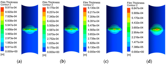
Figure 19.
Film thickness contours of varying lateral pressures. (a) P0.0; (b) P0.1; (c) P0.2; (d) P0.3.
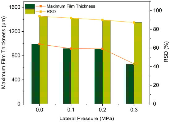
Figure 20.
Maximum film thickness and RSD of varying lateral pressures.
4.2.4. Spraying Distance
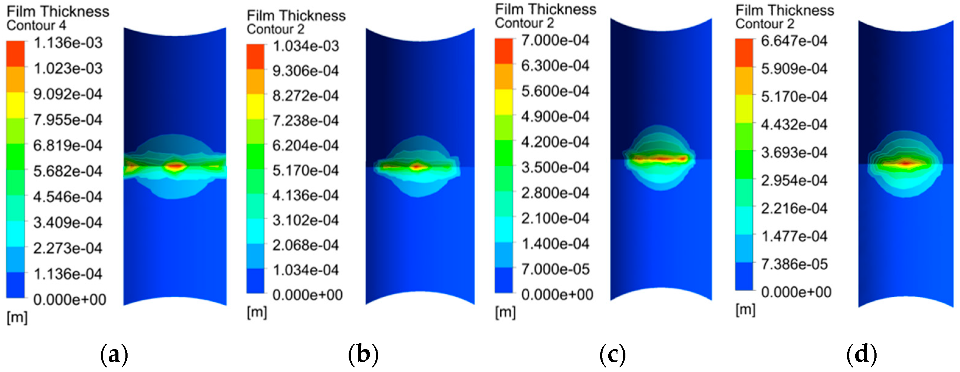
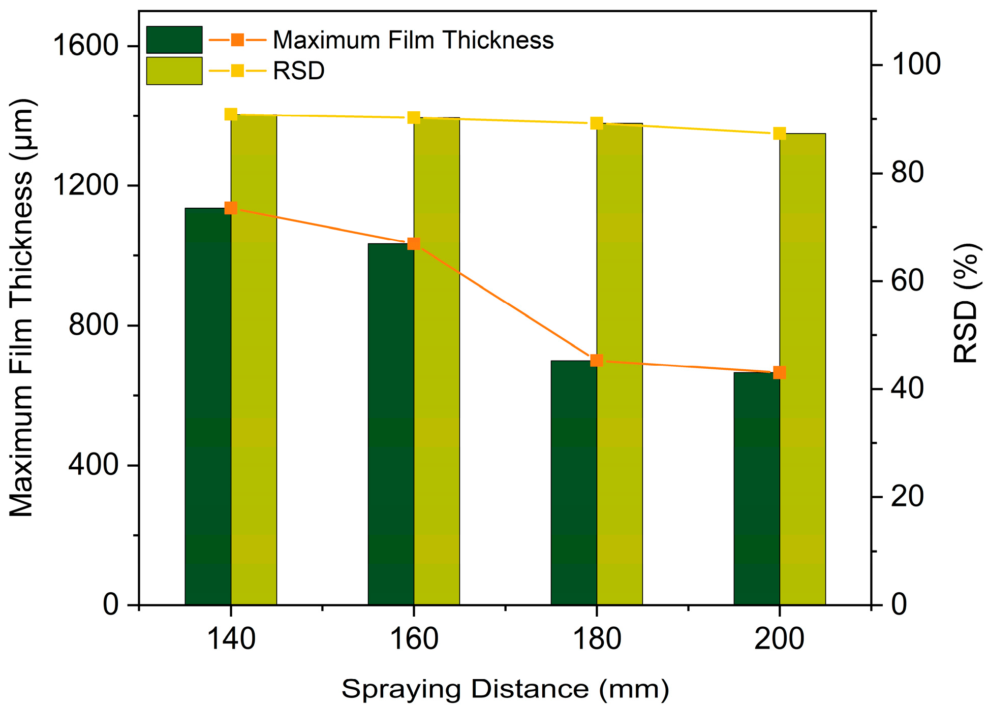
In engineering applications, the spraying distance is often adjusted to accommodate the varying coating requirements of different surfaces. When spraying on UVICS, a long spraying distance will lead to an excessively wide area being covered by the film in a single spray. This will result in a too-thin film that cannot meet the coating requirements, with an attendant uneven thickness at the edges. Consequently, the spraying distances of 140 mm, 160 mm, 180 mm, and 200 mm are selected and designated as L140, L160, L180, and L200, respectively, and the remaining spraying parameters are maintained constant. Subsequently, numerical simulations are conducted, and the resulting film thickness distributions are presented in Figure 21. When the spraying distance is less than 200 mm, the film thickness is distributed with three peaks along the line-through. In contrast, when the spraying distance is 200 mm, the film thickness only exists as one thickness peak. In the X-axis direction, the film widths for the four spraying distances were 150 mm, 140 mm, 121 mm, and 122 mm, respectively. In the Y-axis direction, the film lengths were 138 mm, 140 mm, 150 mm, and 153 mm, respectively. In conjunction with Figure 8d, it can be demonstrated that as the spraying distance decreases, the length and width of the coating film should have decreased in both the X-axis and Y-axis directions, but the width of the coating film increased in the X-direction. The reason is that the spraying distance is insufficient, resulting in the liquid phase contacting the wall over a short distance, which causes excessive local paint deposition. In addition, due to the setting of the specified shear of the wall, a small amount of liquid film sags along the X-axis of the line-through on both sides of the liquid film, which is also the reason for the appearance of three peaks of the liquid film thickness at the line-through. The maximum film thickness and RSD histograms of the coating films at the four spraying distances are presented in Figure 20. The maximum values of the coated film thicknesses are 1136 μm, 1034 μm, 700 μm, and 664.7 μm, respectively, as shown in Figure 22. Overall, the coating films exhibit a decreasing tendency in thickness with increasing spraying distance. The RSD values are found to be 90.87%, 90.25%, 89.19%, and 87.31%, respectively. This indicates that the uniformity of the coating film was gradually enhanced with the increase in spraying distance. Consequently, when all other spraying parameters are held constant, the optimal coating film effect can be achieved when the spraying distance is set to 200 mm.

Figure 21.
Film thickness contours of varying spray distances. (a) L140; (b) L160; (c) L180; (d) L200.

Figure 22.
Maximum film thickness and RSD of varying spray distances.
4.3. Experimental Validation
Firstly, the images of the coating films sprayed on #0, #1, #2, and #3, in comparison with the simulation results, are presented in Figure 23. Noticeably, orange-peel-like surfaces, sagging, graininess, and locally uneven surfaces did not occur on the coating surface. These images demonstrate that the shape of the coating film matches the numerical simulation results to a high degree, thereby confirming the higher degree of accuracy of the numerical simulation results.
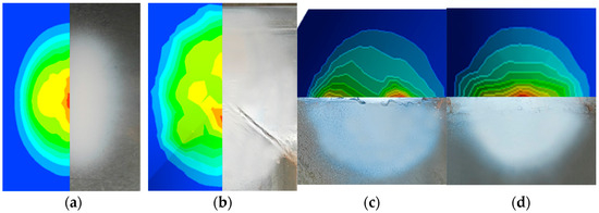
Figure 23.
Simulated and experimental film shapes of varying surfaces. (a) #0; (b) #1; (c) #2; (d) #3.
Since the thickness obtained from numerical simulation is for a wet film, and the thickness of the coating film obtained from experiment is for a dry film it is necessary to convert the wet film thickness to a dry film thickness using the following equation:
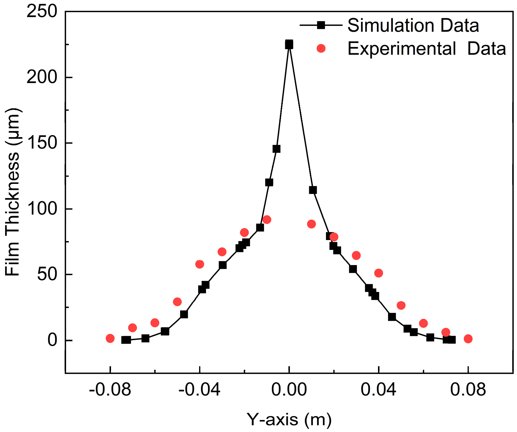
where hd is the dry film thickness, hm is the wet film thickness, η is the coating solid content, and the value of η here is 55%. It is regrettable that when measuring the thickness of the coating film in the area surrounding the line-through, the coating thickness gauge’s probe is unable to measure the line-through due to its unique groove structure. #3 was chosen to measure its coating film thickness in the Y-axis direction. After converting the numerically simulated coating film to dry film thickness, a comparison of the coating film thickness distribution between simulation and experiment is presented in Figure 24. This figure demonstrates that the experimental coating film thickness distribution is in good agreement with the numerical simulation. Within the ±10 mm Y-axis region, the experimental film thicknesses are found to be lower than those of numerical simulations. Conversely, the experimental film thicknesses outside this region are observed to be higher. Furthermore, the experimental film lengths are found to be slightly larger than those of the numerical simulations. The discrepancy between the two measurements can be attributed to the combined influence of gravity and surface tension. During the drying process, the wet film exhibits minor mobility, resulting in a slight lateral movement of the center of the coating film.

Figure 24.
Film thickness distribution curves of simulation and experiment along the Y-axis of #3.
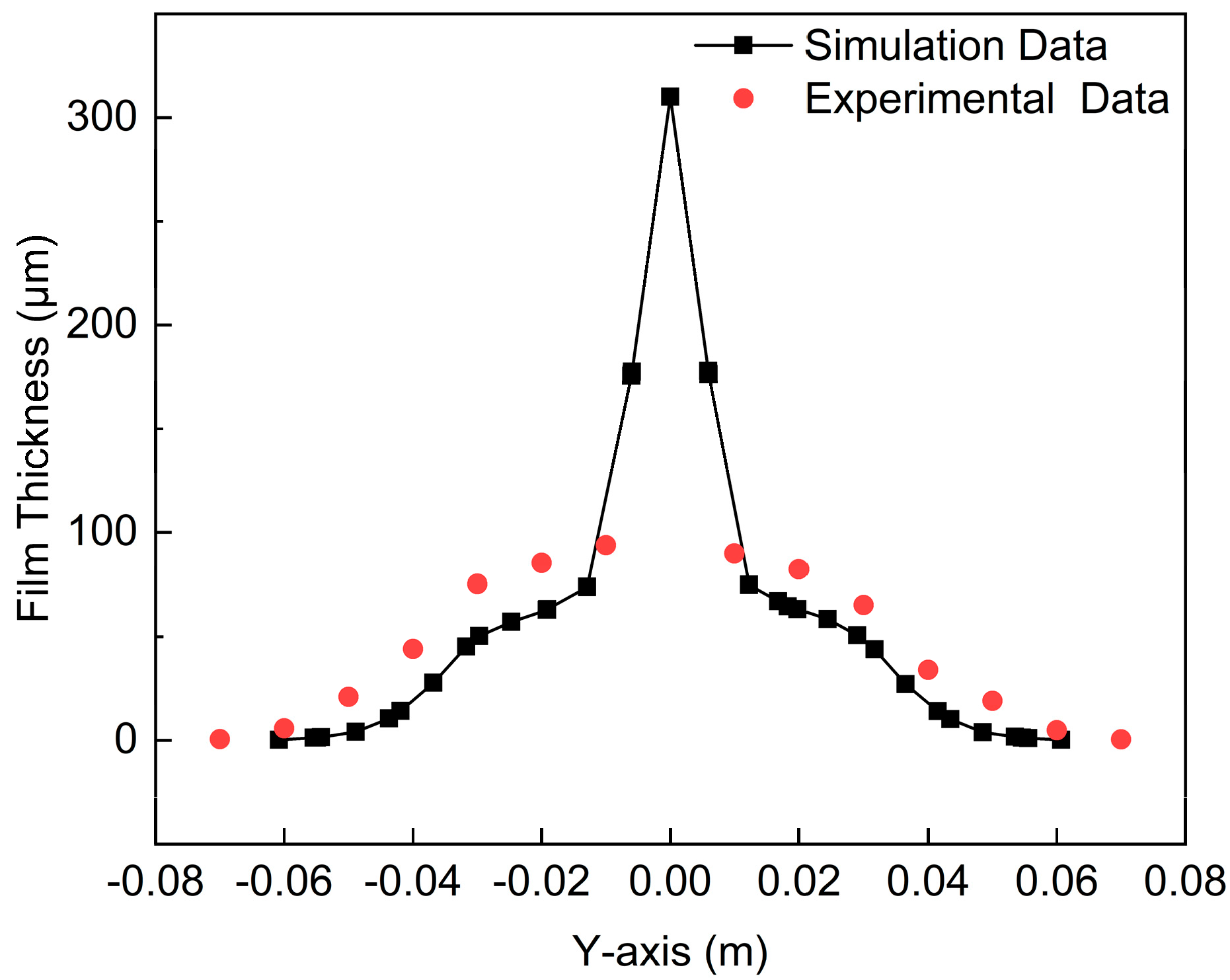
Moreover, the outcomes of the comparison between the spraying experiment and the simulation under varying lateral air pressures when spraying on #3 are illustrated in Figure 25. These figures demonstrate that the overall shapes of the coating film obtained from the experiment and the numerical simulation are nearly identical. P0.3 was chosen to measure the experimental coating film thickness along the Y-axis. Subsequently, compare and analyze the experimental data with the numerical simulation data, as illustrated in Figure 26. Similarly, due to the minor mobility of the paint, the experimental film thickness is lower than the numerical simulation in the region of ±10 mm along the Y-axis, while the experimental film thicknesses outside this region are higher, and the experimental film width is slightly larger than that of the numerical simulation. Overall, the experimental coating film thickness distribution is in good agreement with the numerical simulation, which proves the accuracy of the numerical simulation results.
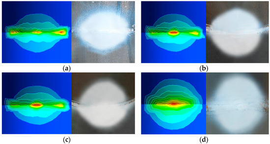
Figure 25.
Simulated and experimental film shapes of varying pressures. (a) P0.0; (b) P0.1; (c) P0.2; (d) P0.3.
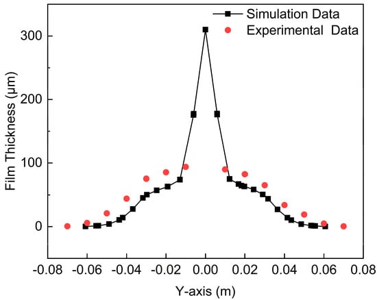
Figure 26.
Film thickness distribution curves of simulation and experiment along the Y-axis of P0.3.
5. Conclusions
In this paper, by modeling the film formation process when spraying on UVICS, corresponding numerical simulations based on CFD and experimental verification were carried out. The film formation characteristics of UVICS were analyzed, and the effects of varying spraying parameters on its film formation characteristics were studied. The main conclusions are as follows:
(1) The numerical simulation results of the UVICS spraying film formation model based on the Euler-Euler approach, as presented in this paper, demonstrate a high degree of agreement with the spraying experimental results, thus demonstrating the accuracy and viability of the model.
(2) The spray flow field characteristics of spraying on UVICS are simulated. In the far-wall spray flow field, the spray flow field is essentially uninfluenced by the shape of the surface features. In the near-wall spray flow field, however, the spray flow field shape, velocity distribution, and pressure distribution are disparate due to the compressing and expanding effects of the surface geometric features on the flow field. The greater the compressing effect of the shape on the flow field, the more pronounced the velocity and pressure gradient in the flow field.
(3) The optimal spraying parameters and the change rule and mechanism of film formation were investigated under various geometric features, dimensions, lateral air pressures, and spraying distances. RSD was employed as a metric for evaluating the film uniformity, and it was found to be satisfactory. The optimal film uniformity for spraying #3 is achieved at a geometric diameter of 100 mm, a lateral air pressure of 0.30 MPa, and a spraying distance of 200 mm, respectively. These results can be utilized to inform the UVICS spraying operation in engineering practice.
Author Contributions
Conceptualization, Y.C.; Data curation, Z.W.; Formal analysis, S.C.; Investigation, J.D.; Methodology, Z.W.; Project administration, J.L.; Software, S.C.; Supervision, Y.C.; Visualization, J.D.; Writing-original draft, Z.W.; Writing-review and editing, Z.W. All authors have read and agreed to the published version of the manuscript.
Funding
This research was funded by the Science and Technology Research Program of Chongqing Municipal Education Commission, grant number [KJZD-M202312901], and the Graduate Research Innovation Program of Chongqing, China, grant number [CYB23299].
Institutional Review Board Statement
Not applicable.
Informed Consent Statement
Not applicable.
Data Availability Statement
Data are contained within the article.
Conflicts of Interest
The authors declare no conflicts of interest.
References
- Zhao, W.; Li, F.; Lv, X.; Chang, J.; Shen, S.; Dai, P.; Xia, Y.; Cao, Z. Research Progress of Organic Corrosion Inhibitors in Metal Corrosion Protection. Crystals 2023, 13, 1329. [Google Scholar] [CrossRef]
- Varela, F.; Tan, M.Y.; Forsyth, M. An overview of major methods for inspecting and monitoring external corrosion of on-shore transportation pipelines. Corros. Eng. Sci. Technol. 2015, 50, 226–235. [Google Scholar] [CrossRef]
- Zgonnik, P.V.; Kuzhaeva, A.A.; Berlinskiy, I.V. The Study of Metal Corrosion Resistance near Weld Joints When Erecting Building and Structures Composed of Precast Structures. Appl. Sci. 2022, 12, 2518. [Google Scholar] [CrossRef]
- Liu, Z.; Cheng, S.; Su, Y.; Duan, G.; Tan, J. Semantic Segmentation Based Spraying Trajectory Planning for Complex Product. IEE Trans. Ind. Inform. 2024, 44, 258–269. [Google Scholar] [CrossRef]
- Yang, X.; Yue, X.; Cai, Z.; Zhong, S. Research on the trajectory planning and global optimization strategy of cold spraying technique for complex products coating preparation. Robot. Intell. Autom. 2024, 44, 258–269. [Google Scholar] [CrossRef]
- Fogliati, M.; Fontana, D.; Garbero, M.; Vanni, M.; Baldi, G.; Donde, R. CFD simulation of paint deposition in an air spray process. JCT Res. 2006, 3, 117–125. [Google Scholar] [CrossRef]
- Pendar, M.R.; Rodrigues, F.; Páscoa, J.C.; Lima, R. Review of coating and curing processes: Evaluation in automotive industry. Phys. Fluids 2022, 34, 101301. [Google Scholar] [CrossRef]
- Ye, Q.; Shen, B.; Tiedje, O.; Domnick, J. Investigations of Spray Painting Processes Using an Airless Spray Gun. J. Energy Power Eng. 2013, 7, 74–81. [Google Scholar]
- Hoppe, F.; Breuer, M. A deterministic and viable coalescence model for Euler–Lagrange simulations of turbulent microbubble-laden flows. Int. J. Multiph. Flow 2018, 99, 213–230. [Google Scholar] [CrossRef]
- Tausendschön, J.; Kolehmainen, J.; Sundaresan, S.; Radl, S. Coarse graining Euler-Lagrange simulations of cohesive particle fluidization. Powder Technol. 2020, 364, 167–182. [Google Scholar] [CrossRef]
- Keser, R.; Battistoni, M.; Im, H.G.; Jasak, H. A Eulerian Multi-Fluid Model for High-Speed Evaporating Sprays. Processes 2021, 9, 941. [Google Scholar] [CrossRef]
- Payri, R.; Gimeno, J.; Martí-Aldaraví, P.; Martínez, M. Validation of a three-phase Eulerian CFD model to account for cavitation and spray atomization phenomena. J. Braz. Soc. Mech. Sci. Eng. 2021, 43, 1–15. [Google Scholar] [CrossRef]
- Domnick, J.; Scheibe, A.; Ye, Q. The simulation of electrostatic spray painting process with high-speed rotary bell atomizers. Part II: External charging. Part. Part. Syst. Charact. 2007, 23, 408–416. [Google Scholar] [CrossRef]
- Zhang, S.; Ma, X.; Hui, Z.; Liu, D.; Yu, G. Numerical simulation study on the effect of voltage on characteristics of spray coating on saddle ridge surface. Electroplat. Finish. 2021, 40, 1856–1864. [Google Scholar]
- Xie, X.; Wang, Y. Research on Distribution Properties of Coating Film Thickness from Air Spraying Gun-Based on Numerical Simulation. Coatings 2019, 9, 721. [Google Scholar] [CrossRef]
- Chen, W.; Chen, Y.; Wang, S.; Han, Z.; Lu, M.; Chen, S. Simulation of a Painting Arc Connecting Surface by Moving the Nozzle Based on a Sliding Mesh Model. Coatings 2022, 12, 1603. [Google Scholar] [CrossRef]
- Chen, S.; Chen, W.; Chen, Y.; Jiang, J.; Wu, Z.; Zhou, S. Research on Film-Forming Characteristics and Mechanism of Painting V-Shaped Surfaces. Coatings 2022, 12, 658. [Google Scholar] [CrossRef]
- Yang, G.; Wu, Z.; Chen, Y.; Chen, S.; Jiang, J. Modeling and Characteristics of Airless Spray Film Formation. Coatings 2022, 12, 949. [Google Scholar] [CrossRef]
- Yang, G.; Chen, Y.; Chen, S.; Zhang, F. Modeling of Film Formation in Airless Spray. J. Phys. Conf. Ser. 2022, 2179, 012024. [Google Scholar] [CrossRef]
- Yi, Z.; Mi, S.; Tong, T.; Li, K.; Feng, B. Simulation Analysis on Flow Field of Paint Mist Recovery with Single Nozzle for Ship Outer Panel Spraying Robot. Coatings 2022, 12, 450. [Google Scholar] [CrossRef]
- Yi, Z.; Mi, S.; Tong, T.; Li, K.; Feng, B.; Li, B.; Lin, Y. Simulation Analysis on the Jet Flow Field of a Single Nozzle Spraying for a Large Ship Outer Panel Coating Robot. Coatings 2022, 12, 369. [Google Scholar] [CrossRef]
- Wu, Z.; Chen, Y.; Liu, H.; Hua, W.; Duan, J.; Kong, L. A Review of the Developments of the Characteristics and Mechanisms of Airless Spraying on Complex Surfaces. Coatings 2023, 13, 2095. [Google Scholar] [CrossRef]
- Gao, Y.; Ierapetritou, M.G.; Muzzio, F.J. Determination of the Confidence Interval of the Relative Standard Deviation Using Convolution. J. Pharm. Innov. 2013, 8, 72–82. [Google Scholar] [CrossRef]
- Koewitsch, I.; Mehring, M. Carbon nitride materials: Impact of synthetic method on photocatalysis and immobilization for photocatalytic pollutant degradation. J. Mater. Sci. 2021, 56, 18608–18624. [Google Scholar] [CrossRef]


Disclaimer/Publisher’s Note: The statements, opinions and data contained in all publications are solely those of the individual author(s) and contributor(s) and not of MDPI and/or the editor(s). MDPI and/or the editor(s) disclaim responsibility for any injury to people or property resulting from any ideas, methods, instructions or products referred to in the content. |
© 2024 by the authors. Licensee MDPI, Basel, Switzerland. This article is an open access article distributed under the terms and conditions of the Creative Commons Attribution (CC BY) license (https://creativecommons.org/licenses/by/4.0/).