Research on the Measurement and Estimation Method of Wheel Resistance on a Soil Runway

Abstract

In view of the fact that there is no suitable measurement method for tire driving resistance during the operation of a transporter on soil pavement, this paper proposes a simple measurement and estimation method for driving resistance on a soil runway based on the Bekker settlement model. In this paper, using the driving resistance equation based on the Bekker model, a simplified equation of driving resistance related to mass is proposed. Using the principle of kinematics, a simple test device for driving resistance was developed, and the test data of the test device were used to determine the parameters of the driving resistance estimation equation of the road surface. The driving resistance of the wheel running state was tested by the simulated aircraft load loading vehicle through the mechanical sensor, and the consistency between the theoretical value and the actual value of the driving resistance value under 8T, 10T, and 12T loads was verified. This research shows that the test method and estimation method have low cost and good accuracy and are suitable for wide promotion. The results of this paper provide a new idea and method for estimating the driving resistance of a wheel when a transporter runs on a soil road and also provide a reference for designing the length of a soil runway.

1. Introduction

The capability of modern transport aircraft to take off and land on unpaved runways represents one of its vital performance indicators. The distance required for these operations on such runways is intimately tied to the resistance encountered by the aircraft on the surface, which is a crucial factor. A relatively comprehensive system has been established for measuring resistance during takeoff and landing on concrete and asphalt pavements. On these surfaces, the primary source of resistance stems from friction; hence, the study of pavement resistance is commonly referred to as skid resistance research, defined as the investigation of friction within the contact zone between tires and the pavement surface [1]. The exploration of pavement skid resistance originated from the broader study of pavement performance, which gained momentum internationally in the 1930s. Early research on skid resistance was primarily initiated in countries experiencing abundant rainfall or frequent snow and ice, where slipping hazards posed significant challenges, thereby necessitating such investigations. The complexity of skid resistance research arises from the myriad of factors influencing the anti-slip performance between tires and road surfaces. From the perspective of the contact system, the primary influences stem from tire properties, pavement characteristics, and surrounding environmental conditions [2]. Specifically, the skid resistance of both concrete and asphalt pavements comprises the following essential components: adhesion and hysteresis [1]. These two components are intimately linked to the micro- and macro-textures of the pavement surface, emphasizing the pivotal role of pavement texture in determining skid resistance. Thus, the study of skid resistance necessitates a comprehensive understanding of these texture characteristics and their interplay with the various factors influencing tire–pavement interaction.

In the past few decades, experts and scholars at home and abroad have proposed many different types of detection equipment and methods. These methods can be divided into direct measurement methods and indirect measurement methods according to the category [3]. The direct approach to assessing pavement skid resistance involves utilizing index parameters that focus on measuring the friction coefficient, a core metric. Conversely, the indirect method revolves around evaluating pavement characteristics and inferring skid resistance based on established conversion relationships, with a primary emphasis on pavement texture analysis. Both methodologies continue to advance through innovation and refinement. One of the earliest methods for testing pavement skid resistance was the vehicle braking distance measurement [4,5]. This straightforward technique involves conducting braking tests on wet roads at 64 km/h, measuring the distance traversed until the wheels lock and the vehicle comes to a halt. It boasted versatility as it could be conducted using regular vehicles, yet its practicality was hindered by limitations in the supporting equipment at the time, leading to a cumbersome process and potential safety concerns. The British Pendulum Test (BPT) [6], introduced by the British Road Research Laboratory in 1964, is a cost-effective and user-friendly tool for evaluating pavement surface friction characteristics. Widely adopted globally, it excels in assessing pavement apparent micro-texture. However, its application is constrained by its inability to cover large areas or perform continuous measurements efficiently. Complementing the pendulum friction tester, the Dynamic Friction Tester (DFT) [7] offers a versatile alternative for low-speed skid resistance assessments. With an extended speed range and the capability for continuous friction monitoring, DFT boasts portability, high efficiency, and swift data processing. Its outcomes can be translated into the International Friction Index (IFI), facilitating standardized comparisons. The Locked-Wheel Skid Trailer [8], prevalent in the United States for both concrete and asphalt pavement evaluations, conducts friction tests on wet surfaces under constant load and a velocity of 64 km/h. It distinguishes itself with its ability to provide continuous friction measurements without disrupting road usage, eliminating the need for lane closures. The Grip Tester [9], a fixed-slip device, specializes in assessing the friction of smooth tires at slip rates ranging from 12% to 20%. Although it delivers precise measurements, its implementation is costly, requiring extensive technician support and significant investment. Lastly, the Mu-Meter [10] represents a versatile lateral force testing solution, capable of assessing a wide array of road conditions, including straight, curved, and steep sections. This equipment underscores the evolution of skid resistance measurement techniques towards more comprehensive and adaptable solutions.

Presently, research on the aircraft running resistance method on soil runways is mainly limited to a series of studies carried out by the United States military. In order to build soil runways for C-17, C-130, and other transport aircraft, the US military used high-speed continuous friction measurement equipment to test the resistance of simple runways. Tingle [11] used a continuous friction test device based on a trailer to perform continuous friction measurements along the direction parallel to a runway in order to develop a soil runway condition level that supports the operation of the C-17 transporter. Ward [12,13] proposed a friction test method for unpaved runway surfaces based on deceleration, which assists in the development of friction prediction models on roads with different humidity conditions and soil types. Based on the above, it can be concluded that many types of detection equipment for concrete and asphalt pavement have been gradually extended to soil pavement. Although there are few case studies on the running resistance of aircraft wheels on soil road surfaces in the field of airport engineering at home and abroad, the research on the interaction between wheels and soil in the field of agricultural and industrial machinery started earlier [14]. Mcallister [15] used a trailer to measure the rolling resistance coefficient of agricultural machinery tires and analyze the influencing factors. Their results showed that tire pressure, vertical load, tire size, and other factors have a great influence on the rolling friction coefficient. Rebati [16] compared the rolling resistance data of different tires with the calculated values of various models and evaluated the prediction accuracy of rolling resistance. They found that the EMOB model was better at predicting cross-layer tires and there was no better model for radial tires. Elwaleed [17] studied the influence of tire pressure on driving resistance and used three different tire pressures to test resistance. The test results showed that the logarithmic model was the best way to describe the movement resistance of agricultural tires. Botta [18] conducted field tests under three soil types, two tire types, and axle load conditions to confirm the relationship between the existing ground pressure parameters and tire shrinkage. The research in the related fields mentioned above studies the resistance of tires on soil road surfaces from various perspectives such as test methods, prediction models, and influencing factors. However, because of the complexity of soil properties, the research conclusions are not universal, and the process is more complicated.

Using a mechanical model of the interaction between aircraft tires and soil pavement based on Bekker theory and its motion equation, this paper explores the driving resistance estimation method of a wheel on a soil runway. The estimation method consists of two important parts. One is to measure the driving resistance of the vehicle based on the kinematics principle, and the other is to estimate the driving resistance of the large-weight aircraft based on the theoretical equation of the driving resistance and the measured driving resistance. This research provides a simple method for estimating tire resistance when an aircraft runs on a soil runway.

2. Theory and Methodology

2.1. Characterization Method of Wheel Resistance on Soil Road Surfaces

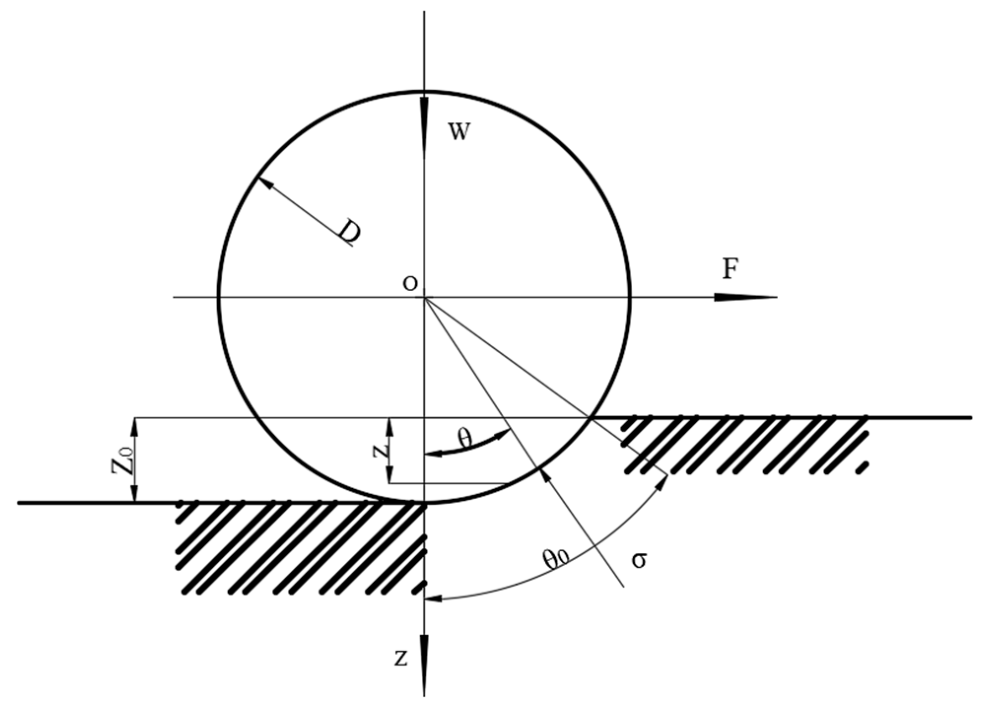
2.1.1. Driving Resistance Characterization Method Based on the Mechanical Model

When a wheel runs on a soil surface, the interaction model between the wheel and soil assumed by Bekker, an American scientist, in the 1960s is usually adopted for analysis [19], and its principle is shown in Figure 1.

In the figure, D is the outer diameter of the wheel, W is the vertical load, F is the driving resistance, Z₀ is the maximum subsidence depth of the tire, z is the subsidence depth, σ is the radial pressure, θ is the angle between the radial pressure and the vertical direction, and θ₀ is the penetration angle of the tire.

For dirt surfaces, pneumatic tires are similar to rigid wheels. Bekker assumed that the reaction force at all points of the surface on the contact area was radial and equal to the normal pressure under the same depth plate in the pressure-subsidence test. According to this assumption, the simplified action model below is drawn to obtain the balance equation of the driven rigid wheel, as shown in Equations (1) and (2):

$$F=b{\displaystyle {\int }_0^{{\theta }_0}}\sigma r\sin \theta d\theta$$

(1)

$$W=b{\displaystyle {\int }_0^{{\theta }_0}}\sigma r\cos \theta d\theta$$

(2)

where F is the driving resistance, b is the tire width, r is the tire radius, σ is the normal pressure, and W is the vertical load.

At the same time, the model satisfies Bekker’s pressure–settlement relationship equation, as shown in Equation (3):

$$p=\left({\displaystyle \frac{k_C}{b}}+k_{\phi }\right)z^n$$

(3)

where p is the pressure, b is the tire width, and n, k_C and k_φ are the parameters describing the pressure–subsidence relationship.

By combining the above relationships and geometric configuration, the driving resistance equation of tire on soil pavement is established, as shown in Equation (4). For the specific derivation process, see reference [20]:

$$F={\displaystyle \frac{1}{{(3-n)}^{\frac{2n+2}{2n+1}}(n+1)b^{\frac{1}{(2n+1)}}\cdot {(k_C/b+k_{\phi })}^{\frac{1}{2n+1}}}}{({\displaystyle \frac{3W}{\sqrt{D}}})}^{{\displaystyle \frac{2n+2}{2n+1}}}$$

(4)

Assuming Equation (5):

$$A={\displaystyle \frac{{(\frac{3g}{\sqrt{D}})}^{\frac{2n+2}{2n+1}}}{{(3-n)}^{\frac{2n+2}{2n+1}}(n+1)b^{\frac{1}{(2n+1)}}\cdot {(k_C/b+k_{\phi })}^{\frac{1}{2n+1}}}}$$

(5)

then, the driving resistance can be characterized as Equation (6):

$$F=A{m}^{{\displaystyle \frac{2n+2}{2n+1}}}$$

(6)

In Equation (6), n can confirm the value based on consulting relevant data. A is the comprehensive coefficient affected by factors such as soil characteristics and tire conditions. When the test vehicle and soil conditions are the same, A is a fixed value.

2.1.2. Kinematic Model-Based Driving Resistance Characterization Method

When an aircraft runs on a soil surface, the takeoff and landing processes are typical acceleration and deceleration processes, and the kinematic equation is as shown in Equation (7):

$$S=v^2/2a$$

(7)

where v is the landing speed or departure speed, S is the landing or takeoff distance, and A is the acceleration. In actual aircraft operation, whether takeoff or landing, this is a variable acceleration process, which is often simplified to a uniform acceleration or deceleration process in the calculation process.

Taking the landing process of an aircraft as an example, according to Newton’s second law, the resistance F = ma encountered by an aircraft during operation is composed of two parts, road surface resistance and air resistance. This paper mainly studies the resistance from the road surface, that is, the wheel driving resistance. From the perspective of kinematics, the resistance can be characterized as Equation (8):

$$F=m{v}^2/2S$$

(8)

2.2. Field Testing of Driving Resistance Based on the Mechanical Model

Bekker’s classic model is an empirical equation, which is mainly applicable to the scenario of inflatable tires on soil surfaces. In order to verify the accuracy of its application in the calculation of aircraft drag on soil runways, a specific site is selected, a soil runway is built, and a simulated aircraft loading vehicle is used to carry out field tests.

2.2.1. Basic Conditions of the Test Site

The test site is located in Baqiao District, Xi’an, Shaanxi Province, with an altitude of about 420 m, and the soil is sticky soil. The Xi’an area has a temperate subhumid continental monsoon climate and is hot and rainy in summer, thundery and windy weather, cold and dry in winter. The test time was from early June to early July, during which the weather is hot, the average temperature is 31 °C, the highest temperature is more than 40 °C, and the precipitation is less, which is suitable for field tests. The test section site is shown in Figure 2.

The depth treatment of the structural layer of the pavement is 30 cm. Because there is no bad geological condition in the original foundation, there is no need to treat the original foundation. Humus is cleaned during construction, and debris such as stones and plastics also need to be removed. The soil in this test section is of good quality and is directly compacted after removing impurities. In terms of the compaction process, the compaction degree reaches more than 90% after a 30T heavy roller is used to vibrate the compaction surface 6 times.

2.2.2. Test Method

(1)

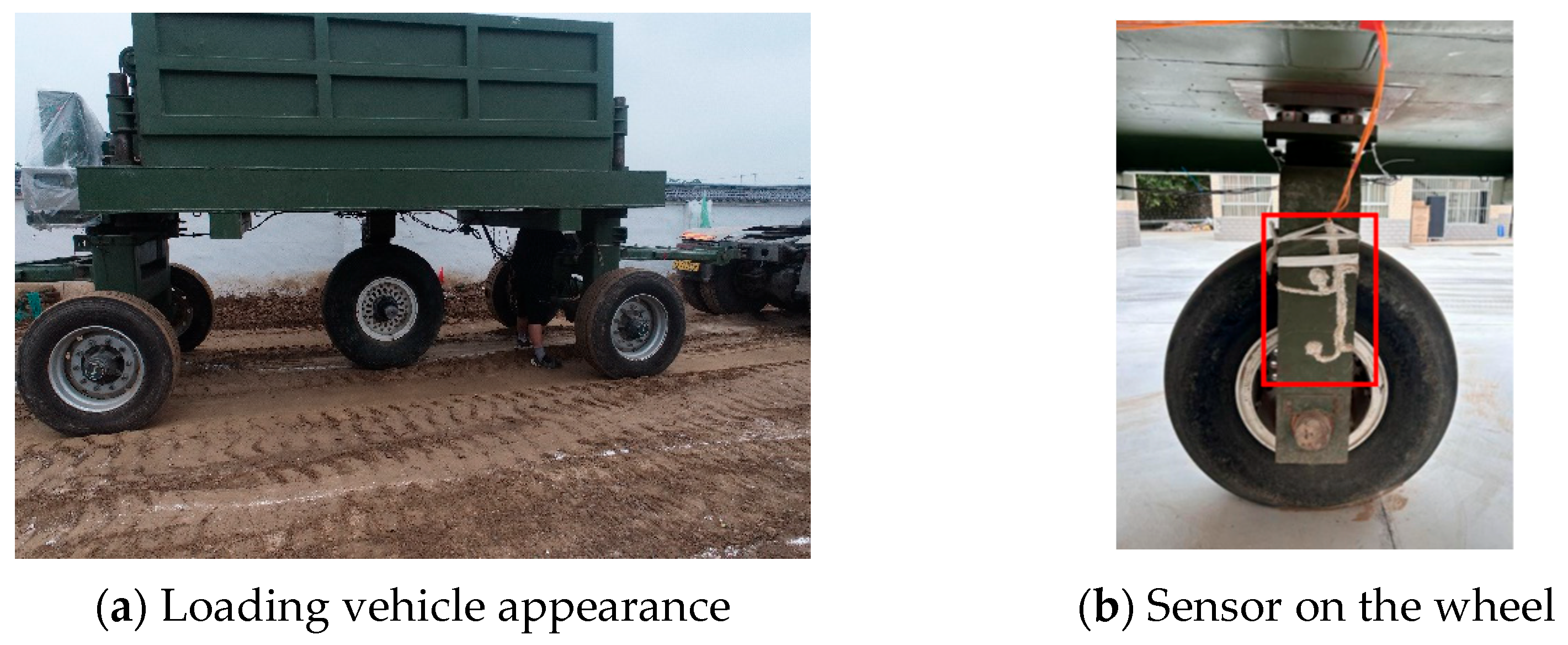
Test equipment

Simulate loading vehicle equipment.

Traffic tests were carried out using a simulated aircraft loading vehicle [21]. The aircraft simulation loading vehicle can simulate the aircraft load, with a self-weight of about 70 kN, equipped with 10 kN weight blocks, up to 200 kN. In the loading process, it can realize step-by-step loading. Figure 3a shows the simulation aircraft load-loading vehicle.

The tension sensor is installed on the bearing wheel, and the heading force is tested by the sensor. The sensor is installed on the central air tire (see Figure 3b) to monitor the direction and force of the tire in real time.

(2)

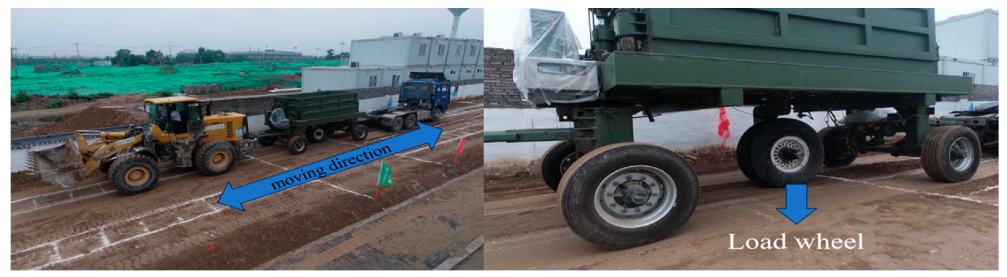
Test process.

Starting from one end of the test section, a tractor is used to make the aircraft load simulate the loading vehicle pass through the test section at a constant speed at a speed of 10 km/h. The weight of the loading vehicle is set to 8T, 10T and 12T respectively, and the same weight is tested 10 times. During the test, the sampling frequency is 10 Hz, and the force in the forward direction is obtained directly through the sensor. The site diagram of the aircraft load simulation loading vehicle is shown in Figure 4.

In this test, it was found that the rut depth did not change significantly after 10 tests, so the test times were set to 10 times.

2.3. Field Test of Driving Resistance Based on the Kinematic Model

According to the kinematics equation, as long as the mass, speed, and distance of the object in the process of movement are measured, acceleration can be inversely calculated, and then the driving resistance can be obtained. According to this principle, the test scheme was designed as follows.

2.3.1. The Test Principle of Speed and Distance

By determining the change rule of the position of the object with time, the running speed and distance can be calculated. At present, the most commonly used position measurement tool is the satellite positioning system. During the test, the satellite positioning system was used, as shown in Figure 5 The model was GPS320 (see Figure 5a), which supports the full-band signals of GNSS’s four systems (GPS, GLONASS, BDS, GALILEO). The antenna positioning is accurate to the millimeter level. The lower part of the antenna is equipped with a magnetic chassis, so that the antenna can be stably adsorbed on the object during the test. The main body of the antenna is stably connected to the GPS receiver through the TNC line (see Figure 5b,c).

Through this device, the vehicle speed information received by the GNSS instrument is transmitted to the mobile phone APP, and the image and CSV data are output and presented on the mobile phone APP (see Figure 6). The APP was developed based on the Android operating system and can be run on smartphones. This APP was developed using the Android Studio development tool. The test state is changed by the change curve of speed and time, and the required data such as the deceleration speed and deceleration distance are counted. The interface is shown below. When the test goes through the start, acceleration, stationary, deceleration, and end states, complete data information is formed. This data information includes start time, start deceleration time, end deceleration time, start deceleration speed, total deceleration time, deceleration distance, test time, test state, deceleration speed curve, deceleration distance curve, etc. It also outputs images of deceleration time and deceleration speed and deceleration time and deceleration distance. Digital data information can be output in CSV data format.

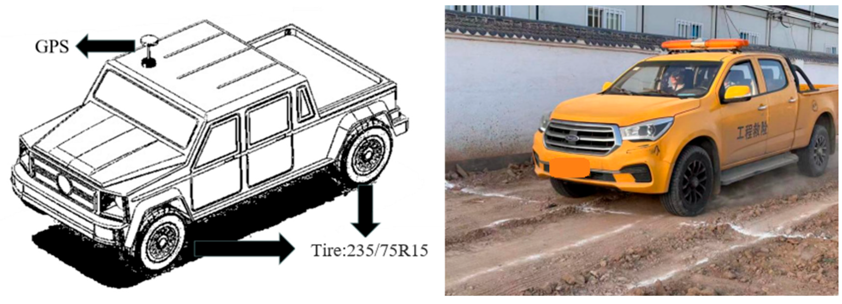
2.3.2. Test Vehicle Selection

This test used the common pickup truck in China as the test vehicle, and the weight of the vehicle is about 2T. The GNSS antenna is installed on the roof of the vehicle, and the signal processor is connected to the power supply in the vehicle to receive the signal. The tire model of the vehicle is 235/75R15, and the tire pressure is 35 psi. The size of the vehicle is shown in Figure 7.

2.3.3. Test Procedure

In the soil field test section established in the second part, the vehicle is set to accelerate from static until the speed reached the predetermined speed, and then the throttle is loosened to allow the vehicle to slide freely forward in a straight line, and finally the speed is reduced to 0 without braking. The vehicle starts from the initial deceleration speed on the test section until the speed drops to 0, which is to complete a complete test. Considering the dispersion of deceleration data and the possible inaccuracy in the device, at least ten repeated measurements were performed for each scene.

3. Results and Discussion

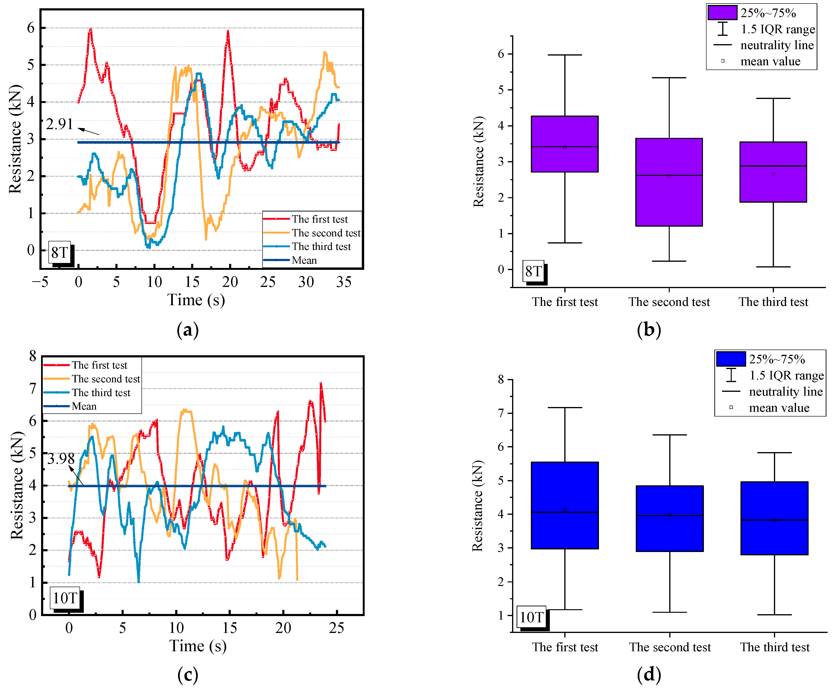
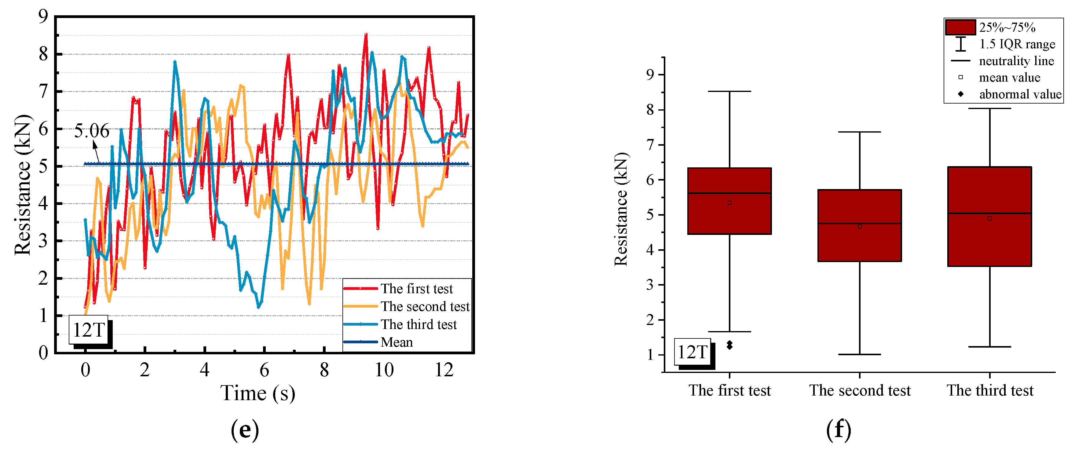
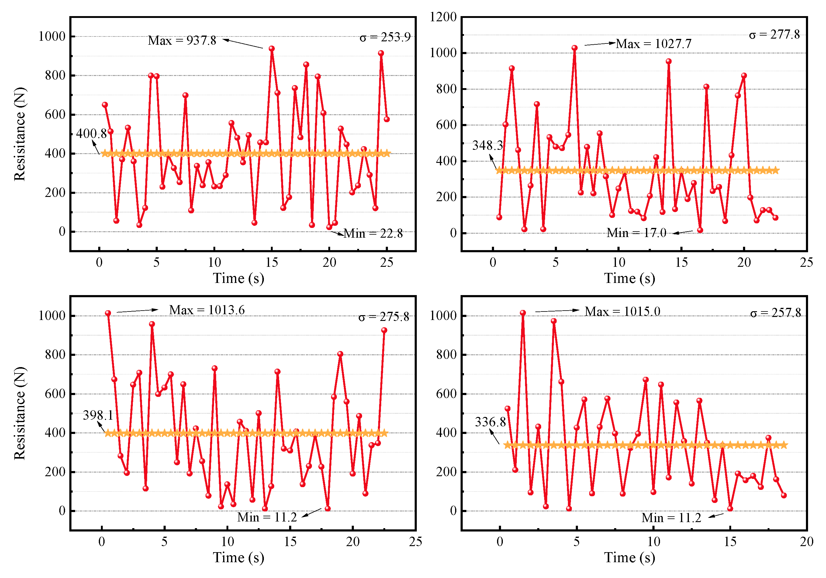
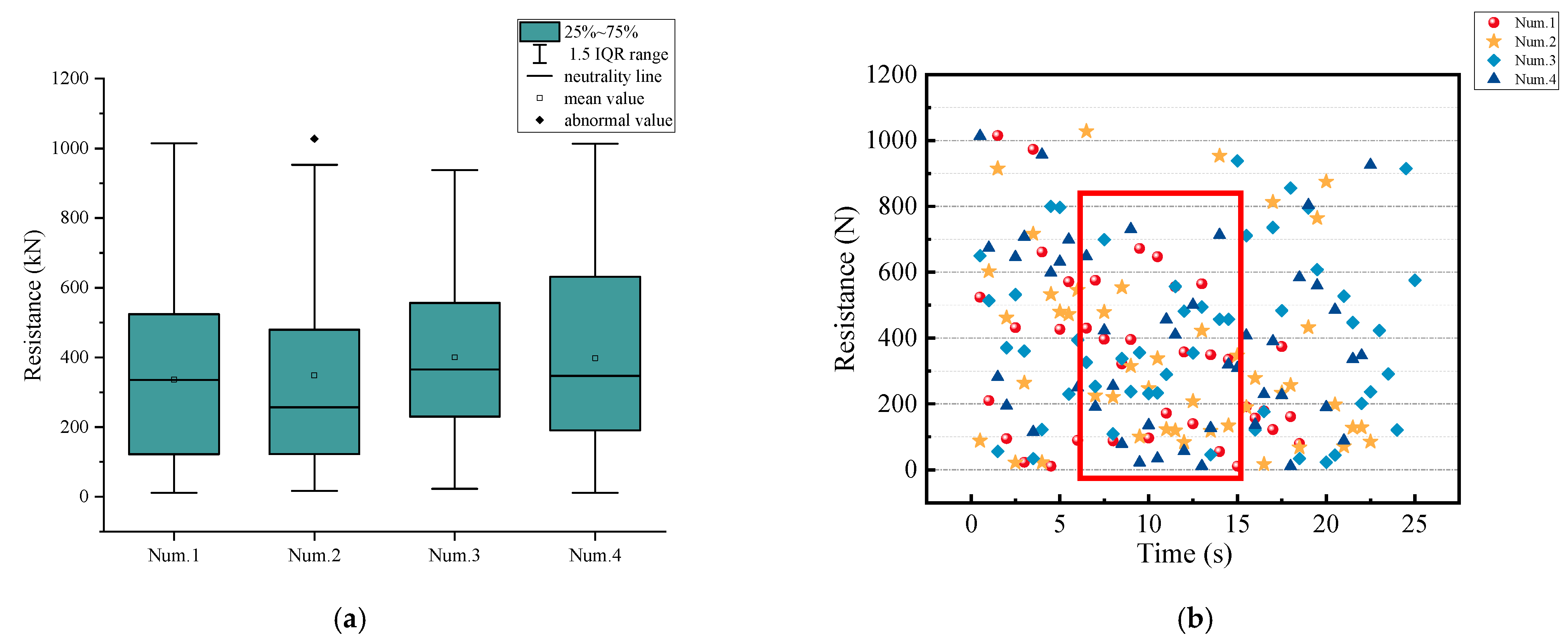
3.1. Test Result Analysis of the Mechanical Model

After the outlier processing of the resistance data obtained from the aircraft load simulation vehicle test, the curve of resistance with time and a box diagram were drawn, as shown in Figure 8. In addition, the standard deviation of each group of data is shown in

Table 1. Driving resistance variance.

	8T			10T			12T
σ	1.16	1.65	1.18	1.42	1.23	1.21	1.51	1.52	1.71
μ	3.39	2.69	2.65	4.14	3.97	3.82	5.35	4.67	4.89

.

The figure shows that the image drawn from the data collected at a sampling frequency of 10 Hz has good continuity. On the soil road surface with a 90% compaction degree, the variation law of road surface resistance under different loading vehicle weight conditions is similar, which fluctuates up and down around a certain value, and the fluctuation range is large, which is also reflected in the box diagram and standard deviation. The variation range of pavement resistance under the three loading conditions is basically between 0 and 6 kN, and most of them are concentrated in the range of 2~5 kN. In addition, with the increase in load, the concentration range of pavement resistance increases gradually, the fluctuation range also increases obviously, and the concentration of data is better. The figure intuitively shows that when the weight of the loading vehicle is 12T, the maximum value of the resistance value exceeds 8 kN, which is higher than the range of the 8T and 10T loads. The average value of the above data was calculated. The average value of the pavement resistance under the weights of the 8T, 10T and 12T loading vehicles shows an upward trend, which is 2910 N, 3978 N, and 5055 N, respectively. In general, although the internal stability of each set of data is poor, the mean value of each set of measured data is relatively stable, and the tested driving resistance is more accurate.

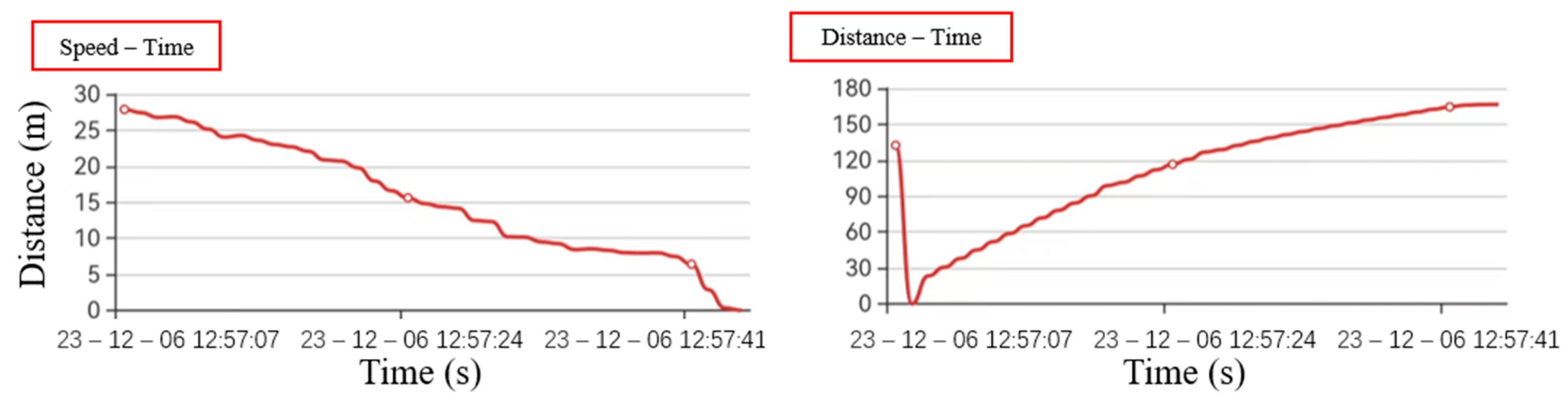
3.2. Test Data Analysis of the Kinematic Model

The data output by the test processing software (Wheel resistance test 1.0) mainly includes the initial deceleration speed, deceleration distance, deceleration time, and so on. The output curve is the curve image of deceleration time and deceleration speed and deceleration time and deceleration distance, as shown in Figure 9.

The test data were recorded at a frequency of 2 Hz, that is, twice per second. In order to facilitate the calculation, the acceleration reduction in the vehicle in the sampling interval remained unchanged, which is a uniform deceleration process. On this basis, the equation is introduced as Equation (9):

$$a={\displaystyle \frac{v^2-{v_0}^2}{2S}}$$

(9)

where a represents the deceleration between the sampling intervals, S represents the distance between the sampling intervals, v represents the speed before the sampling interval, and v₀ represents the speed after the sampling interval.

The deceleration acceleration between the sampling intervals was calculated, and the resistance was obtained by combining Newton’s second law. A total of 10 experiments were carried out in this experiment, and 10 sets of effective data were obtained. In order to reflect the data characteristics more clearly, four sets of data were randomly selected for image analysis. The change in resistance with time is shown in Figure 10, and the resistance box diagram and scatter plot are shown in Figure 11.

The diagram shows that the size of the resistance goes up and down, the overall trend in the fluctuation is stable, and there is no upward trend or downward trend. Because of the difference in the soil compaction degree, the change in soil flatness, the change in the contact condition between tire and soil surface, etc., the resistance of the vehicle will change in the process of moving forward. From the mean value of multiple tests, the mean value of each test dataset is almost equal, and the change in resistance fluctuates up and down around the mean value. Therefore, this paper assumes that this mean value can be used as the resistance value of this test. As shown in the box diagram, the variation range of resistance is 0~1000 N, and most of the data are concentrated between 200 and 700 N. From the time point of view, Figure 11 accurately reflects the characteristics of the change in resistance value. At the beginning and end of the test, the data are more discrete, while the data in the middle (see the red box in Figure 11b) of the test are more concentrated and less volatile. Through the measurement and analysis of multiple sets of data, the average value of multiple measurement data was taken, and the resistance on the compacted soil road surface of the vehicle is 381 N. Although the internal fluctuation of each set of data is large, its mean is relatively stable. The difference between the mean value of each group of data and the mean value of the four groups of data is within 10%, which can reflect the reliability of the measured value.

3.3. Estimation Method of Aircraft Running Resistance on the Soil Road Surface

3.3.1. Determination of the Calculation Parameters of Road Surface Driving Resistance

1.

Principle of parameter determination.

Before using Equation (6) to calculate the driving resistance, two parameters A and n need to be determined. A is determined by the soil characteristics and tires. Relevant scholars [20] have carried out a large number of tests on uniform soil and given the recommended values of parameters such as n, k_C, and kφ under typical soil conditions. According to the recommended values and tire characteristics, A of the corresponding soil and tire can be calculated, and n can be determined according to the type of soil. The results of relevant scholars show that Equation (6) is reasonable in calculating the driving resistance of tires. However, in the actual use process, the soil environment is complex, and it is difficult to be consistent with the working conditions of the recommended parameters. Therefore, it is very important to determine the accurate parameters for the calculation of the driving resistance of aircraft tires on a soil runway.

According to reference [20], n can be determined according to the type of soil, then A can be characterized as Equation (10):

$$A={\displaystyle \frac{F}{m^{\frac{2n+2}{2n+1}}}}$$

(10)

Corresponding to a certain soil pavement, as long as F under a certain working condition is tested, the corresponding coefficient A can be calculated. Under the action of the tire, the resistance of the tire on the soil with a different compaction degree of the same soil can be calculated, which avoids the error caused by the variation in soil parameters and simplifies the calculation method.

2.

Determination of calculation parameters based on the actual test.

Aiming to calculate the driving resistance of the soil road surface, based on the principle of kinematic resistance characterization, the test method established in the fourth part was used to carry out the field resistance test. In this paper, the soil of the test site is clay. According to the literature [20], the n value is 0.5. Under this soil condition, when the compaction degree is 90%, the driving resistance of the corresponding 2T vehicle is 381 N, and the A value is 134.7. Therefore, under the condition of the soil pavement, the calculation equation of the resistance under different vehicle weights without changing the test tire parameters is as shown in Equation (11):

$$F=134.7m^{1.5}$$

(11)

Corresponding to the given soil road, especially the temporary soil simple road, the vehicle weight can also be estimated by this equation. If the resistance caused by the weight is greater than the traction provided by the engine, the vehicle cannot pass.

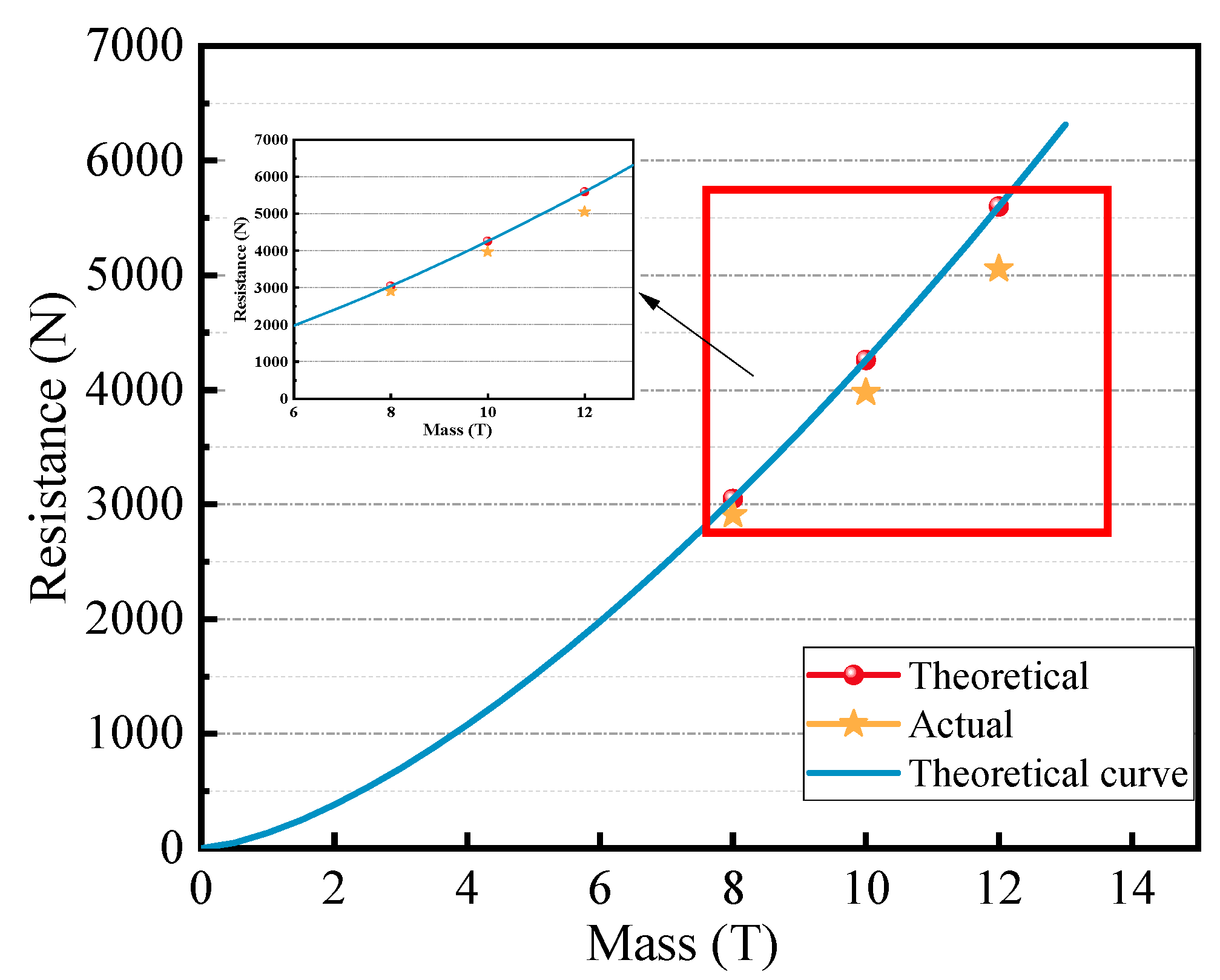
3.3.2. Estimation of Road Surface Driving Resistance

The idea of estimating the driving resistance of the road surface is as follows: for the same soil runway, according to the similarity principle, based on the kinematic equation, the resistance of the vehicle on the road surface is tested by vehicle motion, and then, the vehicle driving resistance is used to estimate the aircraft driving resistance. This method will produce a certain error. The error comes from the difference between the size of the aircraft tire and the size of the test vehicle. Different tires will cause differences in coefficient A. Ignoring the influence of this error, this idea was applied to estimate the driving resistance of the road surface. Taking the data in this paper as an example, considering the single wheel loads of 8T, 10T and 12T, the corresponding wheel driving resistance is calculated as 3048 N, 4260 N, and 5600 N by applying the equation $F=134.7m^{1.5}$.

3.3.3. Accuracy Analysis of the Estimation Method

In the second part of this paper, the pavement resistance under different single wheel loads was tested on site. The comparison between the test data and the estimated value is shown in the

Table 2. Data comparison analysis table.

y = 134.7x1.5
Mass	Theoretical Value	Actual Value	Degree of Deviation
8T	3048	2910	4.53%
10T	4260	3978	6.62%
12T	5600	5055	9.73%

and Figure 12.

The table above shows that the deviation between the actual value and the theoretical value is less than 10%. The driving resistance affects the length of the soil runway. According to the calculation equation in reference [22], the error of the resistance is 10%, and the error in the sliding distance caused by the error is within the range of 50 m, which meets the requirements of the calculation accuracy of the runway length. This shows that the estimation method established in this paper meets the requirements of estimating the driving resistance of the soil pavement.

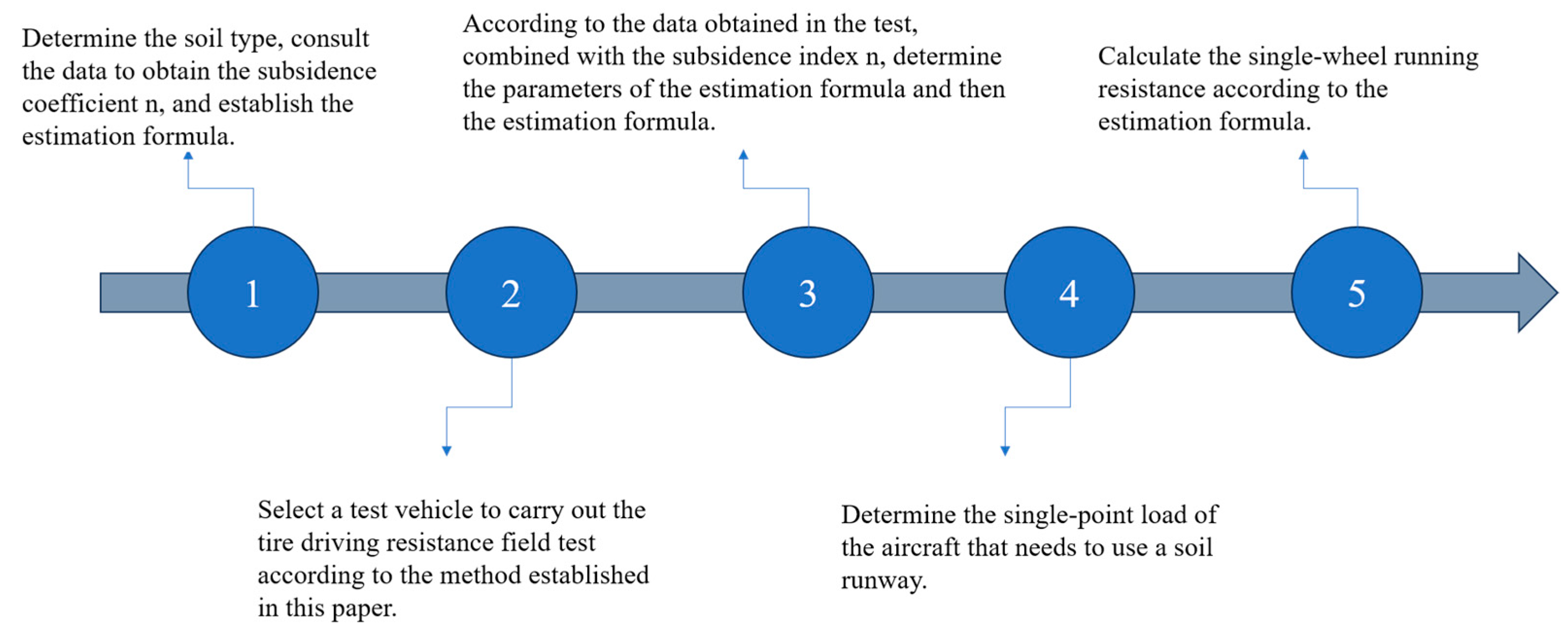
3.3.4. The Process of Estimating the Driving Resistance of Soil Pavement

Based on the idea of this paper, for a given soil runway, the process shown in Figure 13 can be used to estimate the resistance of a single wheel during aircraft operation.

4. Conclusions

Aiming at the complexity of determining wheel running resistance when an aircraft operates on a soil road surface, this study conducts a field resistance test based on tire operation characteristics and establishes an estimation method for aircraft tire running resistance. The following conclusions are drawn:

(1)

Different methods can be used to characterize the driving resistance of the wheel on a soil road surface. Corresponding to different characterization methods, the driving resistance can be tested in two ways as follows: the stress state and the motion state.

(2)

The tire resistance test method based on the motion state can better test the driving resistance of the tire on the soil road. This method can also be used to evaluate the load that the vehicle can bear on temporary soil roads.

(3)

The resistance of the aircraft simulated load-loading vehicle is 2910 N, 3978 N, and 5055 N, respectively, when the single wheel load of 8T, 10T, and 12T is run on the soil pavement. The results obtained by the estimation method established in this paper are 3048 N, 4260 N, and 5600 N, and the deviations are 4.53%, 6.62%, and 9.73%, respectively. These small deviations indicate that our proposed resistance estimation method is feasible for practical application in estimating aircraft tire running resistance.

References

- Mataei, B.; Zakeri, H.; Zahedi, M.; Nejad, F.M. Pavement Friction and Skid Resistance Measurement Methods: A Literature Review. Open J. Civ. Eng. 2016, 6, 537–565. [Google Scholar] [CrossRef]
- Tan, Y.Q.; Xiao, S.Q.; Xiong, X.T. Testing Technology of Dynamic Road Friction. J. Traffic Transp. Eng. 2021, 21, 32–47. [Google Scholar] [CrossRef]
- Gui, Z.; Liu, H.; Zhang, Z. Research Progress of pavement texture Characterization and anti-skid performance detection technolog. Highw. Traffic Sci. Technol. Appl. Technol. Ed. 2012, 4, 62–65. [Google Scholar]
- Eubanks, J.J.; Haight, W.R.R.; Malmsbury, R.N.; Casteel, D.A. A Comparison of Devices Used to Measure Vehicle Braking Deceleration; SAE Technical Paper; SAE: Detroit, MI, USA, 1993. [Google Scholar] [CrossRef]
- Kordani, A.A.; Rahmani, O.; Nasiri, A.S.A.; Boroomandrad, S.M. Effect of Adverse Weather Conditions on Vehicle Braking Distance of Highways. Civ. Eng. J. 2018, 4, 46–57. [Google Scholar] [CrossRef]
- Lee, Y.P.K.; Fwa, T.F.; Choo, Y.S. Effect of Pavement Surface Texture on British Pendulum Test. J. East. Asia Soc. Transp. Stud. 2005, 6, 1247–1257. [Google Scholar]
- Zhang, P.; Cui, L.L.; He, L.; Xia, Q.S. Testing Technology of Dynamic Road Friction Coefficient. Appl. Mech. Mater. 2013, 312, 249–253. [Google Scholar] [CrossRef]
- Rizenbergs, R.L.; Burchett, J.L.; Napier, C.T. Skid-Test Trailer: Description, Evaluation and Adaptation; Commonwealth of Kentucky Department of Highways: Frankfort, KY, USA, 1972. [Google Scholar]
- de Solminihac, H.; Chamorro, A.; Echaveguren, T. Procedure to Process, Harmonize and Analyze Grip Tester Measurements. In Proceedings of the 7th International Conference on Managing Pavement Assets, TRB Committee AFD10, Calgary, AB, Canada, 23–28 June 2008. [Google Scholar]
- Rufford, P.G.; Gaughan, R.L. A Study of the Effect of Speed on the Skid Resistance of Fine and Coarse Textured Surfacings Using the Mu Meter. In Proceedings of the 7th Australian Road Research Board (ARRB) Conference, Adelaide, Australia, 21–25 May 1974. [Google Scholar]
- Tingle, J.S.; Norwood, G.J.; Cotter, B. Use of Continuous Friction Measurement Equipment to Predict Runway Condition Rating on Unpaved Runways. Transp. Res. Rec. 2017, 2626, 58–65. [Google Scholar] [CrossRef]
- Ward, A.B.; Falls, A.J.; Rutland, C.A. Development of Deceleration-Based Friction Prediction Models and Methods on Semiprepared Runway Surfaces. Transp. Res. Rec. J. Transp. Res. Board 2023, 1, 1–16. [Google Scholar] [CrossRef]
- Ward, A.B.; Tingle Jeb, S.; Rutland, C.A. Development of Deceleration-Based Runway Friction Measurement Methods; US Army Engineer Research and Development Center, Geotechnical and Structures Laboratory: Tampa, FL, USA, 2019. [Google Scholar]
- Thompson, R.J.; Visser, A.T. Mine Haul Road Maintenance Management Systems. J. South Afr. Inst. Min. Metall. 2003, 103, 303–312. [Google Scholar]
- McAllister, M. Reduction in the Rolling Resistance of Tyres for Trailed Agricultural Machinery. J. Agric. Eng. Res. 1983, 28, 127–137. [Google Scholar] [CrossRef]
- Rebati, J.; Loghavi, M. Investigation and Evaluation of Rolling Resistance Prediction Models for Pneumatic Tires of Agricultural Vehicles (Research Note). Iran Agric. Res. 2006, 24, 77–88. [Google Scholar]
- Elwaleed, A.K.; Yahya, A.; Zohadie, M.; Ahmad, D.; Kheiralla, A.F. Effect of Inflation Pressure on Motion Resistance Ratio of a High-Lug Agricultural Tyre. J. Terramechanics 2006, 43, 69–84. [Google Scholar] [CrossRef]
- Botta, G.F.; Tolon-Becerra, A.; Tourn, M.; Lastra-Bravo, X.; Rivero, D. Agricultural Traffic: Motion Resistance and Soil Compaction in Relation to Tractor Design and Different Soil Conditions. Soil Tillage Res. 2012, 120, 92–98. [Google Scholar] [CrossRef]
- Bekker, M.G. Land Locomotion on the Surface of Planets. ARS J. 1962, 32, 1651–1659. [Google Scholar] [CrossRef]
- Wong, J.Y. Theory of Ground Vehicles; John Wiley & Sons: Hoboken, NJ, USA, 2022; ISBN 1119719704. [Google Scholar]
- Zhang, J.; Xu, W.; Quan, Z.Q.; Wang, J.; Li, J.Y.; Zuo, S.H.; Chen, T.Y.; Wang, Y.L. Design and application of aircraft load simulation loading vehicle. Exp. Technol. Manag. 2023, 40, 141–148+162. [Google Scholar] [CrossRef]
- Wang, Z.H.; Cai, L.C.; Shao, B. Design Method of Military Airfield Runway Length. J. Transp. Eng. Inf. 2007, 5, 67–70+76. [Google Scholar]