Remaining Useful Life Prediction of Rolling Bearings Based on Deep Time–Frequency Synergistic Memory Neural Network

Abstract

Rolling bearings are essential components of a rotating machinery system. Surface imperfections on bearings can alter vibration patterns, and monitoring these changes allows for the precise prediction of the bearing’s remaining useful life (RUL). To address the limitations, such as inadequate sensitivity to features and constrained time–frequency feature extraction capabilities, in conventional methods for predicting the RUL of rolling bearings in the early stages of degradation, this paper introduces a novel predictive framework that combines dynamic weighting mechanisms with hybrid deep learning. This framework incorporates a continuous wavelet transform to generate two-dimensional time–frequency feature maps as degradation indicators, employs CNN for extracting local detailed features, integrates iTransformer modules with dynamic weighting mechanisms to enhance the focus on early subtle features, and leverages the time-dependent modeling capabilities of BiLSTM. The experimental findings using truncated samples from IEEE-PHM2012 datasets show a 71.82% reduction in errors compared with traditional CNN in the early prediction stages, where it effectively mitigated the challenge of early degradation features being overshadowed by noise. Ablation experiments on model components further validated the effectiveness of the model architecture design, where the dynamic weighting mechanism contributed significantly (29.92%) to improving the mean absolute error (MAE).

1. Introduction

Rolling bearings, a crucial mechanical component widely utilized in rotating machinery, are susceptible to various failures, such as surface cracks, wear, and fatigue spalling, owing to intricate operating conditions, combined loads, and material degradation over time [1]. These failures often manifest as subtle signals early on that are challenging to detect using conventional methods but significantly impact the overall performance of precision machinery. The remaining useful life (RUL) of a mechanical system spans from its initial operation to failure occurrence. By employing sensors or external testing tools to monitor the equipment status during operation, real-time monitoring and forecasting of the RUL can facilitate the development of effective maintenance strategies to prevent failures, ultimately enhancing the machinery longevity and reliability [2].

Mechanical vibration plays a crucial role in equipment operation. As the rolling element traverses the crack surface or wear debris of the bearing, the bearing undergoes a corresponding displacement, leading to the generation of pulse signals manifested in the vibration signal [3]. This, in turn, alters the overall vibration pattern of the bearing. Unlike temperature and friction torque signals, vibration signals exhibit real-time and dynamic characteristics that encompass time–frequency domain degradation features. The vibration amplitude follows a nonlinear progression during wear development, exhibiting gradual accumulation during the initial stages, followed by accelerated growth as the damage propagates. Characteristic fault frequencies (such as raceway defect frequencies) and their associated harmonics/sidebands show progressive amplification with advancing degradation. The enlargement of localized defects enhances the modulation phenomena, leading to increasingly intricate spectral compositions. These inherent properties make vibration analysis particularly valuable for RUL prediction in rolling bearing applications. However, due to the strong nonlinear and time-varying relationships between these features and the RUL, conventional physical models struggle to characterize dynamic degradation mechanisms under multi-fault coupling.

Early methods for predicting the bearing RUL utilizing machine learning algorithms, like a support vector machine (SVM) [4,5,6] and artificial neural network (ANN) [7], have been constrained by their reliance on artificial feature engineering and inadequate generalization capabilities. Deep learning technology has enabled data-driven feature extraction methods to demonstrate significant advantages [8,9,10]. Convolutional neural networks (CNNs) have emerged as a leading approach for multi-scale automatic feature extraction at the feature representation level. Previous studies [11,12,13] enhanced the feature recognition efficiency under complex conditions by refining the network structure. For instance, Akpudo et al. [14] utilized kernel principal component analysis to achieve a monotonic characterization of degradation trends, while Zhang et al. [15] established a more robust feature space using an autoencoder. However, these approaches primarily concentrate on the isolated analysis of local time-domain or frequency-domain characteristics, neglecting the comprehensive modeling of time–frequency coupling characteristics in vibration signals.

Recently, researchers have increasingly utilized recurrent neural network (RNN) architectures to account for the temporal dependence of the degradation process. Guo et al. [16] enhanced the RNN health index method, Lin’s team [17] incorporated the attention mechanism to optimize the gating unit, Zhao et al. [18] combined CNN and bidirectional LSTM to create a spatiotemporal feature extractor, and Yang et al. [19] achieved the dynamic optimization of feature weights using multi-head self-attention. Additionally, Liu et al. [20] integrated domain-adaptive technology into the LSTM network, leading to a significant enhancement in the prediction accuracy across various working conditions. Despite these advancements, the conventional RNN architecture still faces challenges in handling feature space correlation. Consequently, Li et al. [21] developed a graph convolution network that integrates multi-domain data. Wang et al. [22] proposed a temporal graph convolution model, and Cao et al. [23] introduced an equidistant-feature-mapping TCN model, all of which aimed to enhance feature correlation through spatial topology modeling. Zheng et al. [24] developed a deep reinforcement learning (DRL)-integrated framework to mitigate the RUL prediction instability stemming from overlooked temporal dependencies in conventional deep learning approaches by employing an autoencoder for degradation feature extraction coupled with the Twin Delayed Deep Deterministic Policy Gradient (TD3) algorithm to establish temporal state dependencies.

Based on the current research analysis, two primary challenges persist in predicting the remaining useful life (RUL) of rolling bearings. First, many approaches rely on one-dimensional analyses in either the time or frequency domain, and thus, overlook the modal progression of vibration signals across both domains. Second, prevailing temporal models are constrained by local receptive fields and deficient at preserving the memory of initial deteriorating characteristics, leading to model bias when handling extensive datasets over time. Consequently, there is an immediate need to consider the holistic interplay of monitoring vibration signals and exhibit responsiveness to varying dimensions.

A framework is proposed for predicting the early RUL of rolling bearings, comprising the following steps:

• Utilize the continuous wavelet transform to convert scalar vibration signals into 2D time–frequency feature maps.
• Automatically extract features from these time–frequency maps using a multi-layer convolutional neural network.
• Employ an improved inverted Transformer with a dynamic weighted attention mechanism to enhance the model’s performance by effectively capturing the global dependencies within the sequence data.
• Leverage a bidirectional long short-term memory (BiLSTM) network to capture the bidirectional dependencies of the time series, enabling the accurate prediction of the remaining lifespan of rolling bearings.

While a convolutional neural network excels at capturing local features across various scales, they often overlook contextual information. On the other hand, a Transformer is adept at modeling global dependencies but struggles with local spatial contexts and smaller sample sizes. To address these limitations, this study introduces an enhanced iTransformer that mitigates the deficiency of global dependence through a dynamic weighted mechanism, enhancing the interpretability in variable dimensions. Additionally, by incorporating a BiLSTM network to process both forward and backward information, the model’s capacity to comprehend and forecast time series data is further strengthened.

This paper’s follow-up structure is outlined as follows: The second section delineates the fundamental theoretical methodologies associated with the model. The third section clarifies the model’s prediction process and confirms the effectiveness of our model framework by analyzing the open dataset. In the fourth section, assessment metrics are developed, and the model’s performance is demonstrated through ablation study results. Finally, this paper ends by summarizing its results and emphasizing existing limitations.

2. Methods

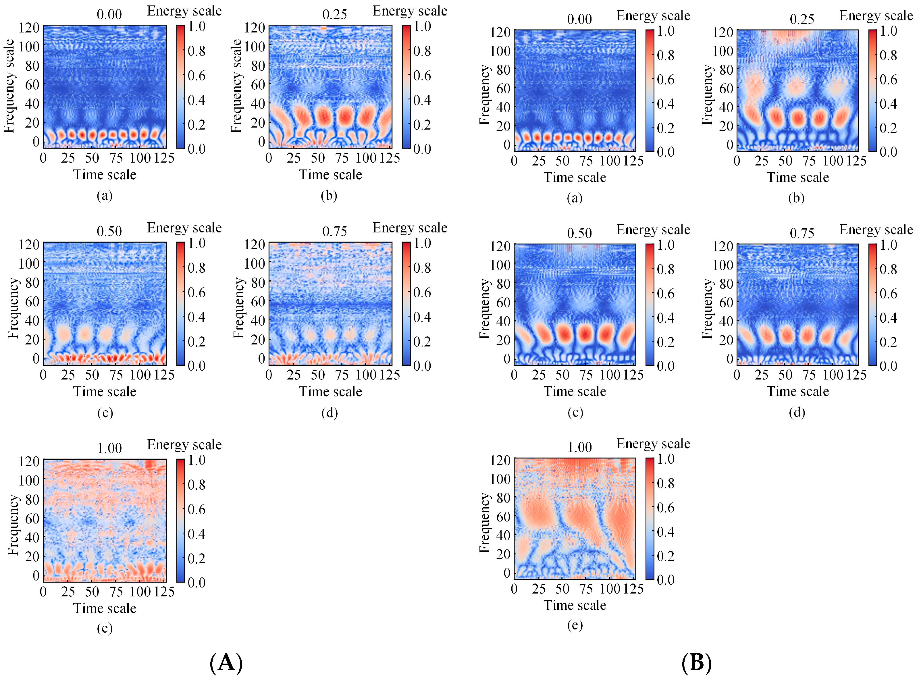
2.1. Continuous Wavelet Transform

The wavelet transform (WT) is a powerful tool for signal analysis. It allows for the decomposition of a signal using a set of wavelet basis functions, enabling the examination of signal characteristics across various scales and positions. This simultaneous analysis of frequency and time information facilitates the processing of non-stationary data. Specifically, the continuous wavelet transform (CWT) assesses signal features by scaling and translating the fundamental wavelet function. Post-CWT, the signal can be represented as Equations (1) and (2):

$$W(a,b)=\int x(t){\phi }_{a,b}^{*}(t)dt$$

(1)

$${\phi }_{a,b}(t)={\displaystyle \frac{1}{\sqrt{a}}}\phi ({\displaystyle \frac{t-b}{a}}),a<0$$

(2)

where $x(t)$ is the search distance; $a$ and $b$ are the scale factor and the time-shift factor; ${\phi }_{a,b}(t)$ is the parent wavelet function; and ${\phi }_{a,b}^{*}(t)$ is the complex conjugate parent wavelet function. The CWT utilizes the parent wavelet function generated through translation and scaling to examine the local features of a signal. The crux of the wavelet transform lies in the choice of the wavelet basis function. Among these, the Morlet wavelet stands out for time–frequency analysis due to its ability to blend the frequency traits of a sine wave with the localization characteristics of a Gaussian window function. This unique combination equips it with a significant advantage in handling signals with periodic and high-frequency features. The Morlet wavelet is expressed as Equation (3) [25]:

$$\psi \left(t\right)=e^{i2\pi {\omega }_{0}t}{e}^{-{\displaystyle \frac{t^2}{2{\sigma }^2}}}$$

(3)

where $t$ represents time; ${\omega }_0$ is the central frequency determining the oscillation frequency of the wavelet; and $\sigma$ is a parameter for wavelet width that controls the temporal span.

To effectively capture the time–frequency attributes of vibration signals, this study employed a continuous wavelet transform to map 1D signals into 2D time–frequency representations. This approach enables the simultaneous visualization of signal time, frequency, and energy on a single graph, thereby augmenting the temporal feature information. Moreover, this method obviates the need for manual feature engineering during implementation and facilitates the automated extraction of pertinent features through subsequent deep learning models.

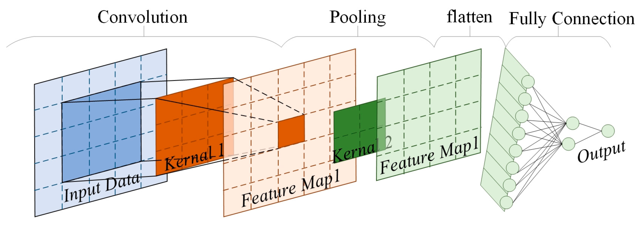
2.2. Convolutional Neural Network

The convolutional neural network (CNN) is a widely used deep feedforward neural network renowned for its proficiency in image data processing. It efficiently leverages time–frequency images derived from a continuous wavelet transform to capture intricate fault characteristics. The structure of a CNN is as shown in Figure 1.

In the CNN model, an input layer receives the original data, while an output layer produces the regression results. The convolution layer, a fundamental component of a CNN, extracts local features from the input data through convolution operations. By sliding the convolution kernel across the input data, a series of feature maps are generated, with each representing a specific feature of the input signal. In RUL prediction, the convolution layer is adept at capturing periodic changes, transient characteristics, and anomalous signals in the data.

Following the convolution layer, the pooling layer downsamples the feature maps to reduce their size while retaining essential information. This study opted for maximum pooling to preserve crucial feature information. Positioned at the network’s end, the fully connected layer merges high-level features from the preceding layers to produce the final output. A CNN effectively captures detailed time–frequency information and automates feature extraction for enhanced RUL prediction.

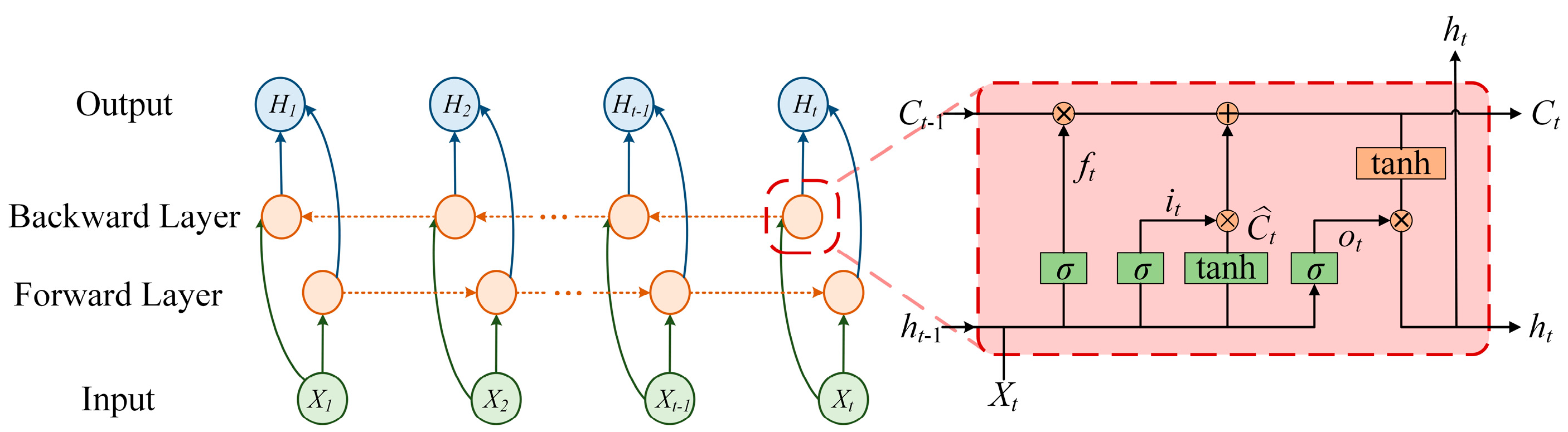
2.3. Bidirectional Long Short-Term Memory Network

Bidirectional long short-term memory network (BiLSTM) is a specialized form of a bidirectional recurrent neural network (BiRNN) [26]. By incorporating gate mechanisms (e.g., input gate, forgetting gate, and output gate) to selectively retain crucial information, LSTM mitigates issues such as vanishing and exploding gradients in the RNN, effectively addressing long-term dependencies. Building upon LSTM, BiLSTM simultaneously handles input sequences using forward and backward layers, allowing for a thorough understanding of temporal information from past and future data. This method aids in extracting initial features from corrupted time series data and improving the prediction accuracy. The schematic representation of BiLSTM is depicted in Figure 2.

The operation of a single LSTM unit in each time step is defined as follows [27]:

$$f_t=\sigma \left(W_f·\left[h_{t-i}{,x}_t\right]+b_f\right)$$

(4)

$$i_t=\sigma \left(W_i·\left[h_{t-1}{,x}_t\right]+b_i\right)$$

(5)

$${\hat{\mathrm{C}}}_t=tanh\left(W_c·\left[h_{t-1}{,x}_t\right]+b_c\right)$$

(6)

$$C_t=f_t·C_{t-1}+i_t·{\hat{\mathrm{C}}}_t$$

(7)

$$o_t=\sigma \left(W_o·\left[h_{t-1}{,x}_t\right]+b_0\right)$$

(8)

$$h_t=o_t·tanh\left(C_t\right)$$

(9)

where $x_t$ represents an input state at a current time step; $h_{t-1}$ denotes a hidden state from the previous time step; $W$ and $b$ are the weight matrix and bias, respectively; and $\mathsf{\sigma }$ signifies the Sigmoid activation function. An input gate $i_t$ regulates whether the information from the current time step is utilized to update a memory unit, while a forgetting gate $f_t$ determines the extent to which historical information is retained in the memory unit. A new candidate state is produced by the candidate memory unit ${\hat{\mathrm{C}}}_t$, and a memory unit state $C_t$ at the current time step is updated by a combination of the forgetting gate and the input gate. Subsequently, a hidden state $o_t$ is computed by the activation value of the memory unit and an output gate, collectively serving as an output $h_t$ for the current time step.

By splicing the forward and reverse hidden states in the feature dimension, BiLSTM constructs a bidirectional feature representation, as depicted in Equation (10):

$$h_t=\left[{LSTM}_{fwd}(x_t,\overrightarrow{h_{t-1}}),{LSTM}_{bwd}(x_t,\overleftarrow{h_{t+1}})\right]$$

(10)

The structural design of BiLSTM enhances feature representation for time series data, particularly during early degradation stages. It also boosts the model’s capacity to handle unknown data and improve generalization.

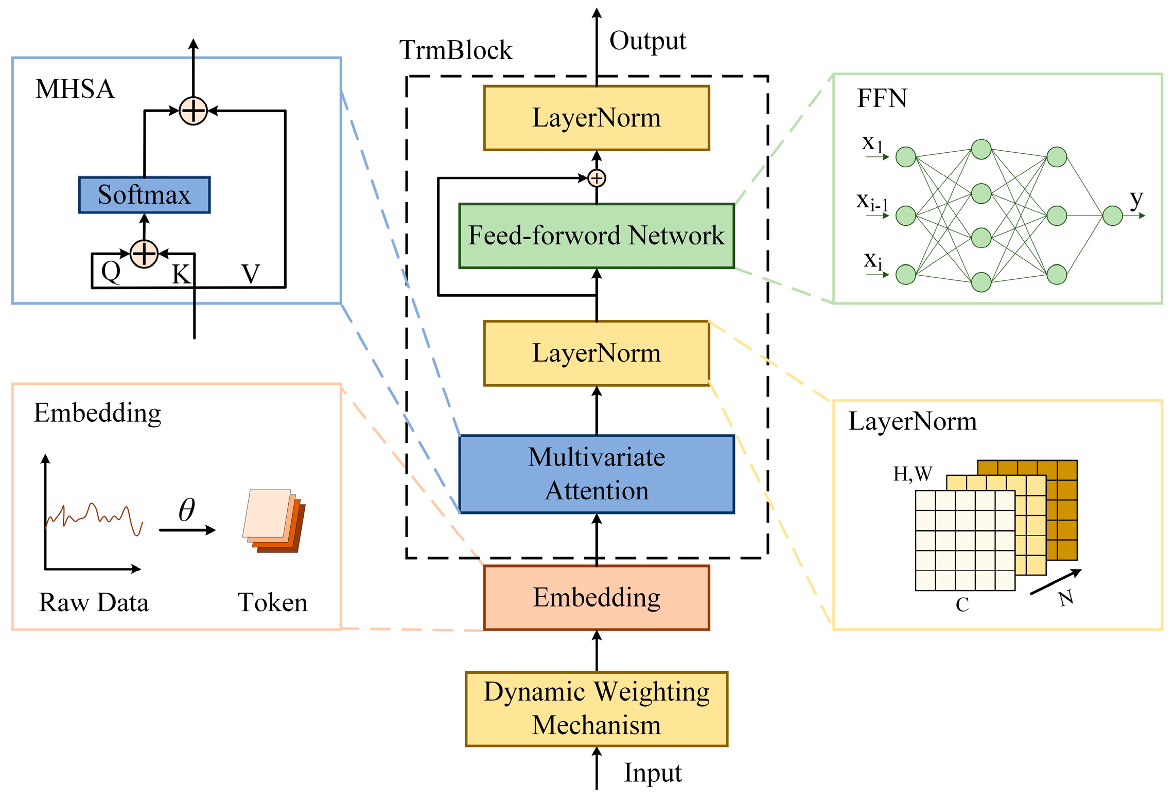
2.4. Optimized Inverted Transformer

The attention mechanism assigns weights based on the input significance, aiding global feature screening to improve the model’s ability to represent the non-linear input–output relationship. To enhance the model’s expressiveness, we propose integrating a dynamic weighting mechanism layer with the inverted Transformer, as shown in Figure 3. The iTransformer [28] comprises Transformer encoder modules that reconfigure the conventional architecture to shift the attention perspective from the temporal dimension to the variable dimension. This is achieved by independently embedding the original data series into token representations of fixed dimensions, enabling a more natural modeling of interactions among multiple variables and a heightened focus on extracting early weak features. The structure, depicted in Figure 3, incorporates key components, including a multivariate attention mechanism, a feed-forward network (FFN), residual connections, and layer normalization.

2.4.1. Dynamic Weighting Mechanism

The dynamic weighting mechanism (DWM) automatically adjusts the allocation of weights for various features based on the dynamic fluctuations in input features. Positioned as an adaptive component between the CNN and iTransformer, the DWM serves to connect local spatial features with global sequence features. By balancing the impacts of both types of features, it enhances the ability to express features and boosts the prediction accuracy. The implementation mechanism of the DWM is as follows:

$$W=Sigmoid\left(MLP\left({GAP(X}_{input}\right)\right)$$

(11)

where $W$ is the weight, and the multi-layer perceptron (MLP) and global average pooling (GAP) are used to achieve dynamic adjustment of the weight matrix.

2.4.2. Multivariate Attention

The multivariate attention, a key component of the Transformer model, is crucial for capturing complex relationships and interactions between features in sequential data. By dividing the self-attention mechanism into several subspaces, the multivariate attention initially conducts input feature mapping [28]:

$$Q=X{W}_Q$$

(12)

$$K=X{W}_K$$

(13)

$$V=X{W}_V$$

(14)

$$Attention\left(Q,K,V\right)=softmax\left({\displaystyle \frac{{QK}^{⊺}}{\sqrt{d_k}}}\right)V$$

(15)

where the query, key, and value matrices, denoted as $Q$, $K$, and $V$, respectively, are derived through a linear transformation of the input sequence. The dimension of the key vector, denoted as $d_k$, is utilized for scaling dot product operations, while $\mathrm{s}\mathrm{o}\mathrm{f}\mathrm{t}\mathrm{m}\mathrm{a}\mathrm{x}$ is employed to compute the weights.

The outputs from multiple attention heads are concatenated and projected back to the original dimension:

$${head}_i=Attention\left(Q_i,K_i,V_i\right)$$

(16)

$$MHSA\left(X\right)=Concat\left({head}_1,{head}_2,...,{head}_h\right)W^O$$

(17)

where $h$ is the number of attention heads and $W^O$ is the projection matrix. In the iTransformer model, the $MHSA$ mechanism is employed to enhance the modeling of dynamically weighted features. This approach improves the ability to capture long-term dependencies and multi-scale information crucial for accurate rolling bearing RUL prediction.

2.4.3. Subsequent Module Design

The following module design maintains the original architecture of the Transformer encoder. A feedforward neural network is utilized for each token, with the ReLU activation function uniformly applied to all tokens to acquire the comprehensive representation of each variable:

$$FFN\left(x\right)=ReLU\left(x{W}_1+b_1\right)W_2+b_2$$

(18)

where $W_1$ and $W_2$ and $b_1$ and $b_2$ are the weight matrices and biases.

LayerNorm normalization is applied after each coding layer to expedite the training and enhance the training stability. By combining the input and output of each layer to create a residual, the issue of vanishing gradients in deep networks can be mitigated.

$$LayerNorm\left(H\right)=\left\{{\displaystyle \frac{h_n-Mean\left(h_n\right)}{\sqrt{Var\left(h_n\right)}}}\left|n=\mathrm{1,2},...,N\right.\right\}$$

(19)

$$Output=LayerNorm\left(x+FFN\left(x\right)\right)$$

(20)

The iTransformer innovation lies in its shift from modeling across the time dimension to the variable dimension. It employs a self-attention mechanism and feedforward network to capture the correlations between multiple variables and global time series features, respectively. While retaining the fundamental Transformer components, iTransformer’s architectural redesign enhances its suitability for time series prediction tasks by overcoming traditional methods’ limitations in global modeling. The dynamic weighting mechanism generates weights that indicate variable importance. Additionally, the model’s computational complexity is reduced, thereby enhancing the operational efficiency.

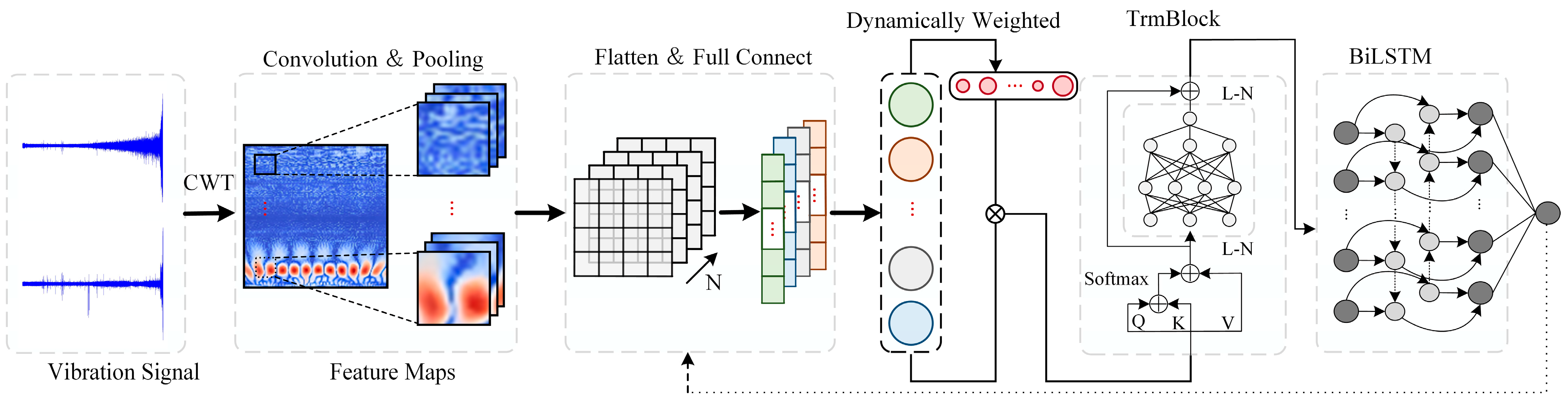
2.5. Model Composition

To address the long-term dependencies in rolling bearing vibration signals, this paper proposes a Time–Frequency Collaborative Dynamic Weighted Memory Network for RUL prediction. The model first employs a CNN to extract deep-level features from input 2D time–frequency (T-F) feature maps. These features are subsequently fed into a dynamic weighting mechanism layer to assign adaptive weights, followed by an iTransformer encoder to model global temporal dependencies. The enhanced features are then processed through a BiLSTM network to capture bidirectional long-term temporal relationships. Finally, the fused representations are transmitted to fully connected layers for bearing RUL prediction. The model framework is illustrated in Figure 4.

The algorithm of our proposed method is shown in

Table 1. Algorithm of method steps.

Algorithm of Model Steps
Input: T-F feature X ∈ ℝN×L×C×H×W
Output: RUL Tag Y ∈ ℝN×1
1. Reshape X to Xreshape ∈ ℝN×L×(C×H×W)
2. Pass Xreshape through CNN Fcnn ← CNN_CWT_Encoder(Xreshape)
3. Feed Fcnn into MLP to generate weights W = MLPθmlp(Fcnn), W ∈ ℝN×L
4. Perform element-wise multiplication Fweighted ← Fcnn⊙W
5. Reshape Fweighted to sequence format Fseq∈ℝN×L×128
6. Pass Fseq through Transformer Ftf ← TransformerEncoder(Fseq)
7. Feed Ftf into bidirectional-LSTM Flstm ← BiLSTM(Ftf)
8. Extract the final time step from Flstm and pass through FC Fout ← FC(Flstm[:, L−1, :])
9. Apply Sigmoid to Fout Y ← Sigmoid(Fout)
10. Return Y

.

3. Simulation Case Verification

3.1. Test Data Presentation

This study utilized experimental validation data from the IEEE-PHM2012 [29]. Multiple identical bearing models were tested within these settings, where vibration signals were captured from the bearing outer ring’s horizontal and vertical axes with acceleration sensors. The horizontal signal represented the vibration measurements in the radial direction of the bearing, which exhibited high sensitivity to radial loads and radial faults (e.g., outer ring defects and rolling element failures). Conversely, the vertical signal corresponded to the vibration measurements in the axial direction of the bearing, which demonstrated significant sensitivity to axial loads and axial faults (e.g., inner ring defects and misalignment issues). The test unit collected a 0.1 s vibration signal every 10 s, with a sampling frequency of 25.6 kHz. A total of 17 sets of bearing vibration data were collected under three different load and speed conditions, as detailed in

Table 2. IEEE PHM 2012 Prognostic Challenge dataset.

Conditions	C_1	C_2	C_3
Speed (rpm)	1800	1650	1500
Force (N)	4000	4200	5000
Training set	Bearing 1_1	Bearing 2_1	Bearing 3_1
	Bearing 1_2	Bearing 2_2	Bearing 3_2
Validation set	Bearing 1_3	Bearing 2_3	Bearing 3_3
	Bearing 1_4	Bearing 2_4
	Bearing 1_5	Bearing 2_5
	Bearing 1_6	Bearing 2_6
	Bearing 1_7	Bearing 2_7

.

3.2. Prediction Process

This study’s platform configuration utilized an Intel Xeon Platinum 8352V processor with a 32-core CPU and GPU version 3060. The setup was based on PyTorch 1.8.1 run on Ubuntu 18.04. The prediction process comprised four main steps.

3.2.1. Data Preparation

During the model training, both the horizontal and vertical acceleration signals underwent preprocessing. While the horizontal acceleration signal captures more degradation information, the vertical acceleration signal is valuable in practical scenarios, particularly when the horizontal signal is affected by noise. The data were first smoothed using a weighted moving average (WMA), as shown in Equations (21) and (22):

$${WMA}_t={\displaystyle \frac{{\sum }_{i=t-W+1}^t{w}_i·x_i}{{\sum }_{i=t-W+1}^t{w}_i}}$$

(21)

$$w_i={\alpha \left(1-\alpha \right)}^{\left(i-1\right)}$$

(22)

where $W$ is the window size, set here to $W$ = 20; $w_i$ is the weight of the data point $x_i$; and $\alpha$ is the attenuation factor, set here to $\alpha$ = 0.1. The WMA assigned higher weights to recent data. This design allowed the WMA to sensitively capture the latest changes while maintaining reasonable utilization of historical information. Such a characteristic was particularly suitable for our focus on early degradation characteristics in this study. Furthermore, by adjusting the window size and weight distribution, the WMA achieved a balance between noise suppression and effective signal preservation, thereby avoiding the loss of critical information caused by oversmoothing.

3.2.2. Feature Engineering

The data underwent continuous wavelet transformation using the Morlet wavelet after applying a WMA. The wavelet scale range was defined as 128, and the resulting wavelet coefficients were subsequently manipulated in the following manner:

$$coef={\mathit{log}}_2\left({coef}^2+0.001\right)$$

(23)

$$coef={\displaystyle \frac{coef-{coef}_{min}}{{coef}_{max-}{coef}_{min}}}$$

(24)

The wavelet coefficient was squared to quantify the signal’s energy, followed by a logarithmic compression to reduce the dynamic range for improved numerical stability. Subsequently, the data were normalized, organized into a time–frequency feature matrix, and utilized as a 2D input for the CNN model. For the entire operational lifespan of Bearing 1_1, time–frequency images from five distinct intervals were randomly chosen, as depicted in Figure 6, where Figure 5A shows the characteristic value of the horizontal acceleration signal, and Figure 5B shows the characteristic value of the vertical acceleration signal.

The feature maps depict the time scale on the horizontal axis, frequency scale on the vertical axis, and amplitude energy using a thermometer color map. During the initial operational phase, the bearing’s overall amplitude energy was predominantly concentrated in the low-frequency range, where it exhibited relatively low amplitude levels. As the operation progressed, high-frequency noise emerged, accompanied by a gradual increase in the vibration amplitude. A 2D feature map enables the fusion of three types of information without the loss of partial features seen in conventional feature extraction methods.

3.2.3. Model Training

By iteratively applying convolutional operations, intricate features could be progressively extracted to ensure efficient resource utilization in the four-layer convolutional neural network. Subsequently, the multidimensional data was flattened and then input into two fully connected layers. The parameters of each layer of the CNN are shown in

Table 3. Model parameters for CNN module.

Layer Type	Input Size (C, H, W)	Operation	Output Size (C, H, W)
Conv_1	2, 128, 128	Kernel = 3 × 3; same padding	16, 128, 128
Maxpool_1	16, 128, 128	Kernel = 2 × 2	16, 64, 64
Conv_2	16, 64, 64	Kernel = 3 × 3; same padding	32, 64, 64
Maxpool_2	32, 64, 64	Kernel = 2 × 2	32, 32, 32
Conv_3	32, 32, 32	Kernel = 3 × 3; same padding	64, 32, 32
Maxpool_3	64, 32, 32	Kernel = 2 × 2	64, 16, 16
Conv_4	64, 16, 16	Kernel = 3 × 3; same padding	128, 16, 16
Maxpool_4	128, 16, 16	Kernel = 2 × 2	128, 8, 8
Flatten	128, 8, 8	/	8192
Fc_1	8192	Dropout = 0.5	256
Fc_2	256	Dropout = 0.2	128

.

The eigenvalues generated by the fully connected layer were fed into the subsequent iTransformer model. The inclusion of horizontal and vertical acceleration signals in the input features introduced computational redundancy in the initial prediction phase. To mitigate this, a dynamic weighting mechanism layer was incorporated to assign weights to the input features, which significantly reduced the computational load without compromising essential features. The DWM employed global average pooling (GAP) to extract global feature representations and utilized a multi-layer perceptron (MLP) to automatically generate channel-wise attention weights, which were adaptively optimized through back-propagation within the overall network framework. The weighted sequences were independently embedded into fixed-dimensional token representations before being fed into the iTransformer module for subsequent processing. The iTransformer comprised four stacked encoder layers, each equipped with an independent multi-head self-attention mechanism that featured eight self-attention heads. Additionally, each layer included a feedforward neural network with a hidden layer dimension of 512 and employed dropout regularization (dropout = 0.1). This hierarchical architecture enabled the model to progressively learn intricate feature representations, which enhanced its learning and reasoning capabilities.

The iTransformer encoder module generated features that were fed into the BiLSTM module with a hidden layer dimension of 256 and 2 model layers. The output from the final time step was then processed through a fully connected layer with a Sigmoid activation function to predict the remaining useful life, constrained within the range [0, 1].

To optimize the model training, the chosen loss function was the mean square error (MSE), which aimed to minimize the discrepancy between the predicted value and the actual value by calculating the squared differences. The MSE loss function can be expressed as

$$MSE=\sum _{i=1}^n{\left(\widehat{y_i}-y_i\right)}^2$$

(25)

where $\widehat{y_i}$ and $y_i$ represent the predicted and the actual values of the samples, and $n$ is the number of samples.

The Adams optimizer was utilized for the model training. Given the complexity of the rolling bearing life prediction task, MultiStepLR was implemented to enhance the training efficiency. Specifically, at the 20th, 40th, and 60th epochs, the model’s learning rate was decreased by a specified factor ratio. Additionally, to enhance the training stability and model generalization, a cosine annealing learning rate scheduling strategy was integrated at the 60th epoch during the later stages of training. This strategy effectively decelerated the decrease in the learning rate as the model neared convergence, which facilitated a more refined search for the optimal solution within the parameter space.

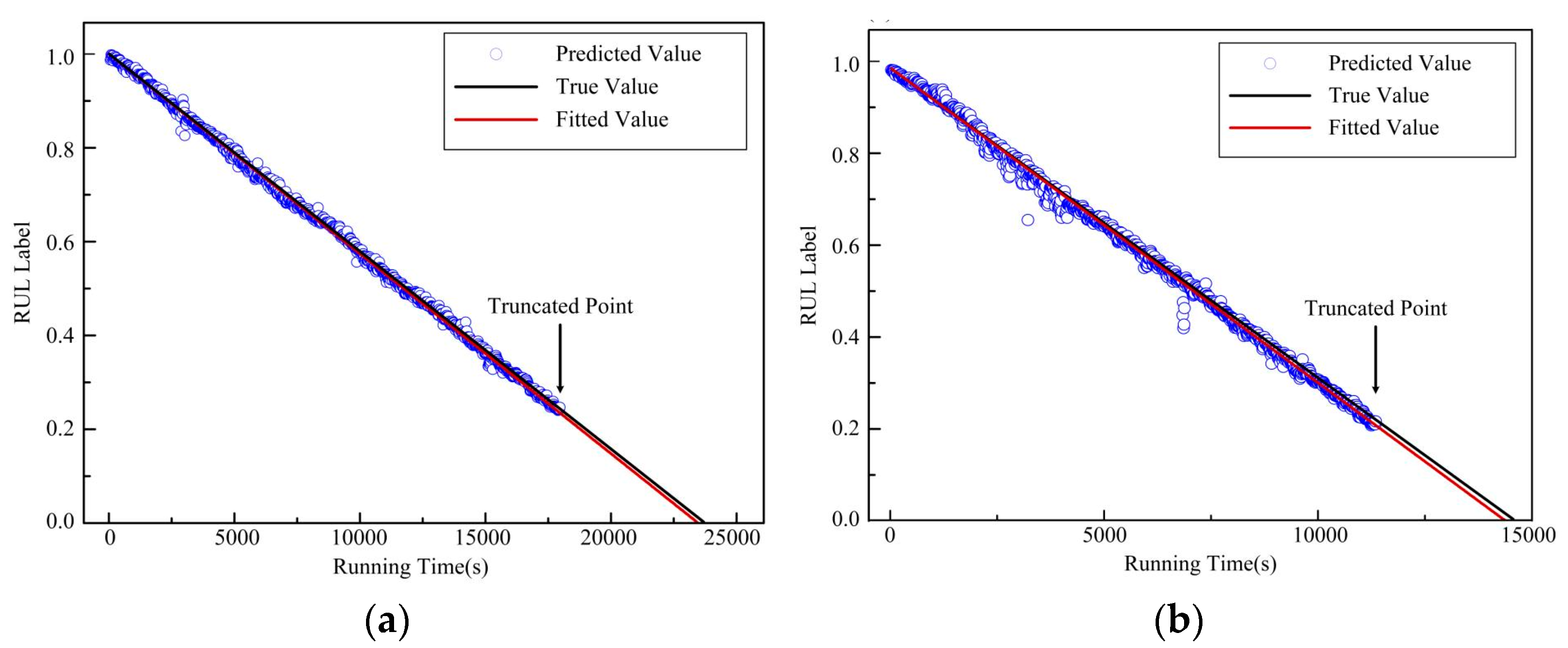
3.2.4. RUL Prediction

We normalized the lifetime labels to [0, 1] and output the fitting results in the validation set, as shown in Figure 6.

4. Results and Discussion

4.1. Evaluation of Model Early Prediction Ability

To evaluate the model’s predictive performance on early-stage degradation indicators, we selected truncated samples from the Test_set of the IEEE-PHM2012 dataset (Bearings 3–7 under condition 1 and Bearings 3–7 under condition 2) to predict their remaining useful life (RUL), as illustrated in Figure 7. By employing a linear function to model the predicted value, we derived the RUL predictions for each truncated sample and subsequently computed the model’s prediction error ($\mathrm{E}\mathrm{r}$):

$${Er}_i={\displaystyle \frac{{ActRUL}_i-{PreRUL}_i}{{ActRUL}_i}}\times 100\%$$

(26)

A positive error indicates a leading prediction, while a negative error signifies a lagging prediction, with a relatively lower average accuracy. Leading predictions offer a higher level of assurance for the overall system safety compared with lagging predictions. The prediction errors are shown in

Table 4. Model prediction error.

Bearing ID	Our Model (%)	CNN (%)	CNN-BiLSTM (%)	CNN-Attention [30] (%)
1_3	0.92	−2.18	−0.87	7.62
1_4	1.88	−4.07	4.50	−157.71
1_5	0.20	−7.69	0.21	−72.57
1_6	0.69	4.15	6.06	0.93
1_7	1.51	−6.94	45.42	85.99
2_3	0.20	−5.51	−1.22	81.24
2_4	4.49	9.20	17.86	9.04
2_5	1.51	6.11	29.58	28.19
2_6	−0.69	−4.08	−0.15	24.92
2_7	−3.41	−5.12	−3.88	19.06
$\overline{\left|{Er}_i\right|}$	1.55	5.50	10.98	40.67

. There are also some other model comparisons presented.

The model demonstrated significant robustness and accuracy in predicting the errors of truncated samples. The model prediction ${Er}_i$ values were all less than 5%, which outperformed the traditional method across the majority of samples. The ${\overline{Er}}_i$ was only 1.55, which decreased 71.82% from the CNN model and 85.88% from CNN-BiLSTM. It also surpassed the method introduced in [30] in terms of the prediction accuracy. Additionally, the model consistently achieved superior predictions in various test sets, which is particularly beneficial for specific engineering applications. This capability aids in preventing faults and enables timely maintenance interventions.

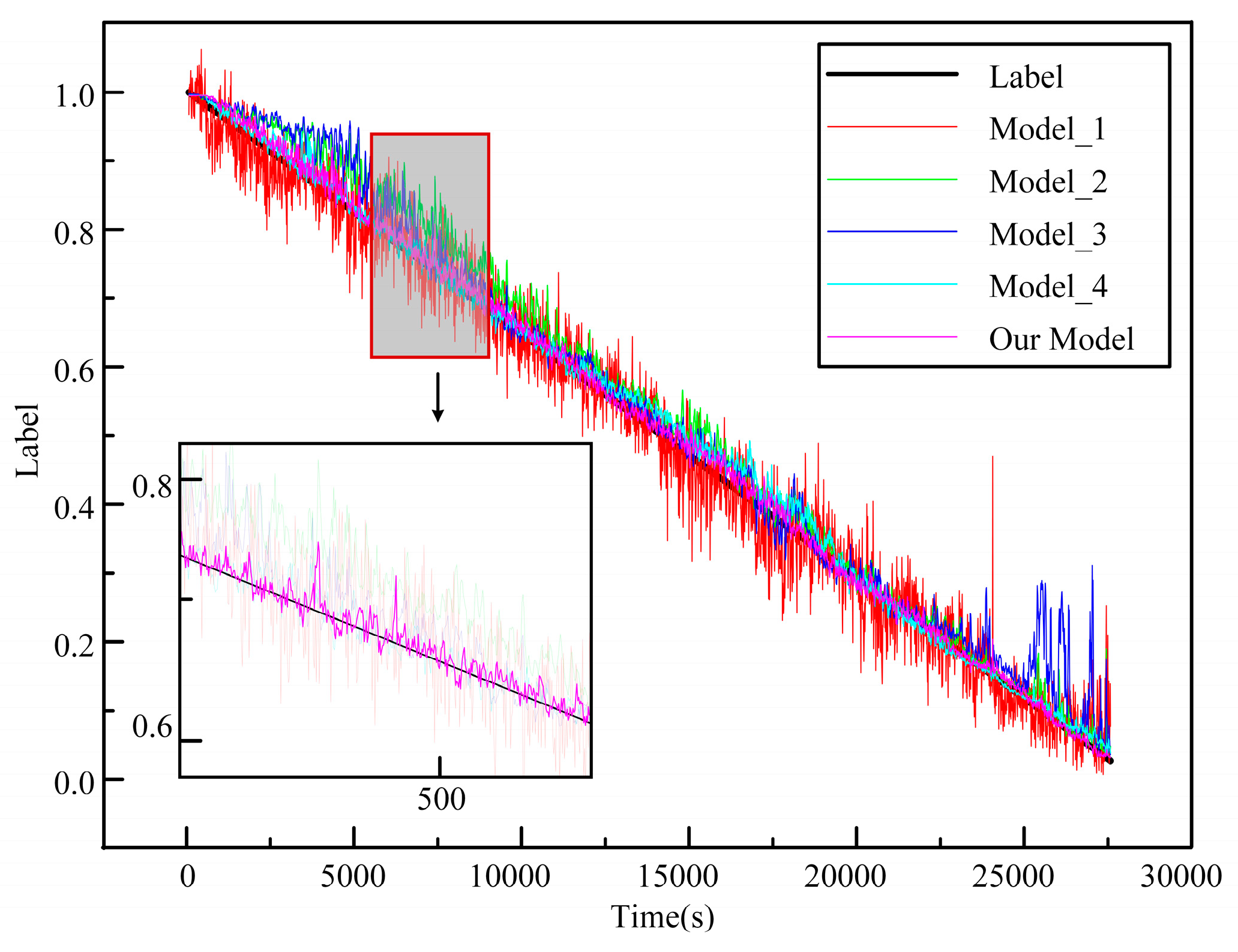
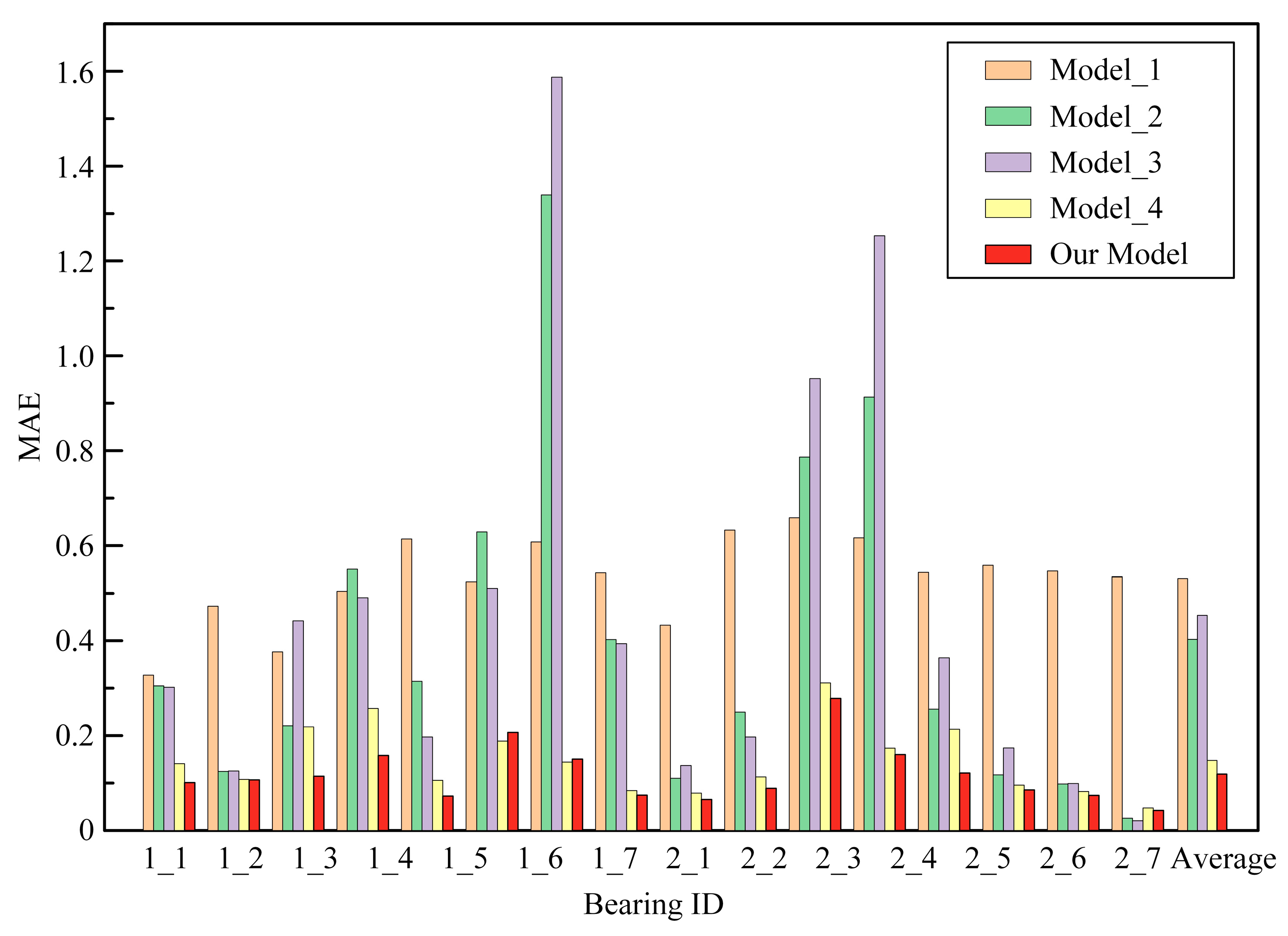
4.2. Comparative Experiment

To further assess the model’s advantages and demonstrate its efficacy, we conducted an ablation experiment that compared the predictive performance of five algorithm models in working conditions 1 and 2 in the PHM2012 dataset. The models evaluated were a four-layer CNN (referred to as Model_1), CNN with LSTM (Model_2), CNN with BiLSTM (Model_3), CNN-iTransformer-BiLSTM (Model_4), and our model. This analysis aimed to investigate the impact of each module design and the dynamic weighting mechanism layer on the model performance. Some of these predictions are shown in Figure 8 and Figure 9. The division of the training set, validation set, and test set was performed on the dataset of the same bearing, with a ratio of 6:2:2.

We verified the validity of the proposed framework by calculating the mean absolute error (MAE) and R² score (R²):

$$MAE={\displaystyle \frac{1}{n}}\sum _{i=1}^n\left|y_i-\widehat{y_i}\right|$$

(27)

$$R^2=1-{\displaystyle \frac{\sum _{i=1}^n{\left(y_i-\widehat{y_i}\right)}^2}{\sum _{i=1}^n{\left(y_i-\overline{y}\right)}^2}}$$

(28)

where $\overline{y}$ is the average value of the actual value. The MAE of each model was calculated and is shown in Figure 10.

Table 5. $R^2$ of prediction results.

Bearing ID	Model_1	Model_2	Model_3	Model_4	Our Model
1_1	0.9785	0.9823	0.975	0.9978	0.9979
1_2	0.9535	0.9969	0.9960	0.9978	0.9978
1_3	0.9707	0.9859	0.9581	0.9388	0.9964
1_4	0.9478	0.9074	0.9484	0.9506	0.9519
1_5	0.9141	0.9772	0.9919	0.9850	0.9982
1_6	0.9396	0.8937	0.9384	0.9430	0.9545
1_7	0.9168	0.5679	0.4501	0.9757	0.9914
2_1	0.9393	0.9209	0.9587	0.9989	0.9989
2_2	0.9633	0.9972	0.9862	0.9991	0.9991
2_3	0.9182	0.9836	0.9919	0.9310	0.9971
2_4	0.9075	0.8631	0.8132	0.9797	0.9310
$2\_5$	0.9134	0.7974	0.6546	0.9905	0.9846
$2\_6$	0.9381	0.9852	0.9703	0.9387	0.9971
$2\_7$	0.9370	0.9966	0.9936	0.9978	0.9979
$\overline{R^2}$	0.9384	0.9182	0.9019	0.9732	0.9835

displays the $R^2$ values for the predictions across each validation set.

The results demonstrate that the four-layer CNN model exhibited subpar performance, where it yielded an $\overline{MAE}$ of 0.74615 across all validation sets. This consistent performance suggests a limitation in early feature extraction and an incapacity to capture global features. Upon integrating the LSTM module, which leverages long-term data dependencies, the model faced challenges stemming from limited data availability in the initial stages or gradient vanishing, which resulted in significant errors in both the early and late stages.

To enhance the model performance, we introduced the BiLSTM module in this study and leveraged its bidirectional propagation to capture forward and backward signal dependencies simultaneously. This approach effectively mitigated the boundary effect issue that arises from unidirectional LSTM dependencies. By incorporating contextual information, BiLSTM bolstered the model’s capacity to grasp sequence-wide features, which led to notable enhancements in both the early and late prediction accuracy.

The integration of the iTransformer module significantly mitigated the model’s boundary effect issue. Utilizing a multi-head self-attention mechanism, iTransformer dynamically captured essential features of sequence signals on a global scale, which enhanced the model’s sensitivity and efficiency in handling the complex time series data, which improved the prediction accuracy.

This study utilized a dynamic weight adjustment strategy that optimized the iTransformer module by dynamically recalibrating the input feature weights. This approach effectively balanced the feature contributions to the target task and significantly enhanced the model’s sensitivity to signal variations, which facilitated the extraction of weak degenerate features in the early stages. The experimental results demonstrate that incorporating the DWM reduced the model’s $\overline{MAE}$ by 29.92%, while the $\overline{R^2}$ improved by 1.06%.

5. Conclusions

This paper introduces a deep time–frequency synergistic memory neural network for calculating the early RUL of bearings. The approach employs a CWT to derive time–frequency images from the input signal, with a CNN facilitating the automatic feature extraction. The iTransformer, augmented by a dynamic weighted mechanism, models global features, while BiLSTM performs the prediction. Utilizing the IEEE-PHM2012 dataset, the method achieved a minimal error in predicting truncated samples, which affirmed its efficacy in early-stage bearing degradation. Comparative experiments revealed a reduction in the average MAE and an increase in the R², which underscored our model’s accuracy in forecasting RUL and its capability to anticipate early failures. This method holds significant promise for engineering applications involving precision rotating machinery.

Current deep learning-based RUL prediction functions as a “black box” model that lacks explicit representation of degradation mechanisms. Building on this study, future research could incorporate a dynamic weighting mechanism to fuse multi-modal data (such as temperature) and account for microscopic surface changes by capturing key characteristic variables. Enhancing the interpretability of the algorithm involves elucidating the impact of microscopic surface alterations on macroscopic mechanical systems. Although the proposed model framework achieved a high prediction accuracy, it also incurred significant computational complexity and extended calculation times. Future work should focus on developing more efficient convolution and attention modules to reduce the computational demands while preserving signal features to facilitate broader engineering applications.

References

1. Ma, M.; Zhang, X.; Tan, C.; Liu, P. Analysis of potential failure modes and failure mechanisms of aerospace components. Yanshan Univ. 2024, 38, 1–9. [Google Scholar] [CrossRef]
2. Spreafico, C.; Russo, D.; Rizzi, C. A state-of-the-art review of FMEA/FMECA including patents. Comput. Sci. Rev. 2017, 25, 19–28. [Google Scholar] [CrossRef]
3. Tandon, N.; Choudhury, A. A review of vibration and acoustic measurement methods for the detection of defects in rolling element bearings. Tribol. Int. 1999, 32, 469–480. [Google Scholar] [CrossRef]
4. Zhe, N.; Yang, J.; Liu, W.; Chen, L. Application of KPCA and improved SVM in rolling bearing remaining life prediction. J. Mech. Eng. 2019, 43, 1–4+8. [Google Scholar] [CrossRef]
5. Lei, Y.G.; Chen, W.; Li, N.P. Adaptive multi-core combined relevance vector machine prediction method and its application in remaining life prediction of mechanical equipment. Mech. Eng. 2016, 52, 87–93. [Google Scholar] [CrossRef]
6. Zhang, M.; Yin, J.; Chen, W. Rolling bearing fault diagnosis based on time-frequency feature extraction and IBA-SVM. IEEE Access 2022, 10, 85641–85654. [Google Scholar] [CrossRef]
7. Wang, X.; Han, Y.; Leung, V.C.M.; Niyato, D.; Yan, X.; Chen, X. Convergence of edge computing and deep learning: A comprehensive survey. IEEE Commun. Surv. Tutor. 2020, 22, 869–904. [Google Scholar] [CrossRef]
8. Lu, B.; Liu, Z.; Wei, H.; Chen, L.; Zhang, H.; Li, X. A deep adversarial learning prognostics model for remaining useful life prediction of rolling bearings. IEEE Trans. Artif. Intell. 2021, 2, 329–340. [Google Scholar] [CrossRef]
9. Ma, M.; Mao, Z. Deep-Convolution-Based LSTM Network for Remaining Useful Life Prediction. IEEE Trans. Ind. Informat. 2021, 17, 1658–1667. [Google Scholar] [CrossRef]
10. Deng, L.F.; Li, W.; Yan, X.H. An intelligent hybrid deep learning model for rolling bearing remaining useful life prediction. Nondestruct. Test. Eval. 2024, 1, 1–28. [Google Scholar] [CrossRef]
11. Xu, Z.F.; Jin, J.T.; Li, C. Fault diagnosis method of rolling bearings based on multi-scale convolutional neural networks. Vibration Shock 2021, 40, 212–220. [Google Scholar] [CrossRef]
12. Meng, Z.; Dong, S.; Pan, X.; Wu, W.; He, K.; Liang, T.; Zhao, X. Fault diagnosis of rolling bearings based on improved convolutional neural networks. Comb. Mach. Autom. Process. Technol. 2020, 2, 79–83. [Google Scholar] [CrossRef]
13. Li, X.; Zhang, W.; Ding, Q. Deep learning-based remaining useful life estimation of bearings using multi-scale feature extraction. Reliab. Eng. Syst. Saf. 2019, 182, 208–218. [Google Scholar] [CrossRef]
14. Akpudo, U.E.; Hur, J.W. A feature fusion-based prognostics approach for rolling element bearings. Mech. Sci. Technol. 2020, 34, 4025–4035. [Google Scholar] [CrossRef]
15. Zhang, T.; Wang, Q.; Shu, Y.; Xiao, W.; Ma, W. Remaining useful life prediction for rolling bearings with a novel entropy-based health indicator and improved particle filter algorithm. IEEE Access 2023, 11, 3062–3079. [Google Scholar] [CrossRef]
16. Guo, L.; Li, N.; Jia, F.; Lei, Y.; Lin, J. A recurrent neural network based health indicator for remaining useful life prediction of bearings. Neurocomputing 2017, 240, 98–109. [Google Scholar] [CrossRef]
17. Lin, R.; Wang, H.; Xiong, M.; Hou, Z.; Che, C. Attention-based gate recurrent unit for remaining useful life prediction in prognostics. Appl. Soft Comput. 2023, 143, 110419. [Google Scholar] [CrossRef]
18. Zhao, G.Q.; Jiang, P.; Lin, T.R. Intelligent rolling bearing remaining useful life prediction method based on CNN-BiLSTM network and attention mechanism. Mech. Electr. Eng. 2021, 38, 1253–1260. [Google Scholar] [CrossRef]
19. Yang, J.; Zhang, X.; Liu, S.; Yang, X.; Li, S. Rolling bearing residual useful life prediction model based on particle swarm optimization-optimized fusion of convolutional neural network and bidirectional long–short-term memory–multihead self-attention. J. Electron. 2024, 13, 2120. [Google Scholar] [CrossRef]
20. Liu, C.Y.; Gryllias, K. Unsupervised domain adaptation based remaining useful life prediction of rolling element bearings. PHM Soc. Eur. Conf. 2020, 5, 10. [Google Scholar] [CrossRef]
21. Li, P.; Liu, X.; Yang, Y. Remaining useful life prognostics of bearings based on a novel spatial graph-temporal convolution network. Sensors 2021, 21, 4217. [Google Scholar] [CrossRef] [PubMed]
22. Wang, Y.; Xu, Z.; Zhao, S.; Zhao, J.; Fan, Y. Performance degradation prediction of rolling bearing based on temporal graph convolutional neural network. J. Mech. Sci. Technol. 2024, 38, 4019–4036. [Google Scholar] [CrossRef]
23. Cao, X.; Zhang, F.; Zhao, J.; Duan, Y.; Guo, X. Remaining useful life prediction of rolling bearing based on multi-domain mixed features and temporal convolutional networks. Appl. Sci. 2024, 14, 2354. [Google Scholar] [CrossRef]
24. Zheng, G.; Li, Y.; Zhou, Z.; Yan, R. A remaining useful life prediction method of rolling bearings based on deep reinforcement learning. J. IEEE Internet Things 2024, 11, 22938–22949. [Google Scholar] [CrossRef]
25. Morlet, J.; Arens, G.; Fourgeau, E.; Glard, D. Wave propagation and sampling theory; Part I, Complex signal and scattering in multilayered media. Geophysics 1982, 47, 203–221. [Google Scholar] [CrossRef]
26. Schuster, M.; Paliwal, K.K. Bidirectional recurrent neural networks. IEEE Trans. Signal Process. 1997, 45, 2673–2681. [Google Scholar] [CrossRef]
27. Greff, K.; Srivastava, R.K.; Koutník, J.; Steunebrink, B.R.; Schmidhuber, J. LSTM: A Search Space Odyssey. IEEE Trans. Neural Netw. Learn. Syst. 2017, 28, 2222–2232. [Google Scholar] [CrossRef]
28. Liu, Y.; Hu, T.; Zhang, H.; Wu, H.; Wang, S.; Ma, L.; Long, M. ITRANSFORMER: Inverted transformers are effective for time series forecasting. arXiv 2023. [Google Scholar] [CrossRef]
29. Nectoux, P.; Gouriveau, R.; Medjaher, K.; Ramasso, E.; Chebel-Morello, B.; Zerhouni, N.; Varnier, C. PRONOSTIA: An experimental platform for bearings accelerated degradation tests. In Proceedings of the IEEE International Conference on Prognostics and Health Management, Denver, CO, USA, 18–21 June 2012. [Google Scholar]
30. Chen, Y.; Peng, G.; Zhu, Z.; Li, S. A novel deep learning method based on attention mechanism for bearing remaining useful life prediction. Appl. Soft Comput. 2020, 86, 105919. [Google Scholar] [CrossRef]
Figure 1. Structure of CNN.
Coatings 15 00406 g001
Figure 2. Structure of BiLSTM.
Coatings 15 00406 g002
Figure 3. Optimized iTransformer structure.
Coatings 15 00406 g003
Figure 4. The model framework.
Coatings 15 00406 g004
Figure 5. Acceleration signal characteristics of Bearing 1_1: (Aa–Ae) horizontal acceleration signal characteristics; (Ba–Be) vertical acceleration signal.
Coatings 15 00406 g005
Figure 6. RUL prediction results: (a) Bearing 1_1; (b) Bearing 1_2; (c) Bearing 1_3; (d) Bearing 2_1; (e) Bearing 2_2; (f) Bearing 2_3.
Coatings 15 00406 g006
Figure 7. Fitted RUL prediction results: (a) Bearing 1_3; (b) Bearing 1_4.
Coatings 15 00406 g007
Figure 8. Bearing 1_1 prediction contrast.
Coatings 15 00406 g008
Figure 9. Bearing 1_3 prediction contrast.
Coatings 15 00406 g009
Figure 10. MAE of prediction results.
Coatings 15 00406 g010