A Dynamic Collision Risk Assessment Model for the Traffic Flow on Expressways in Urban Agglomerations in North China

Abstract

Expressways in urban agglomerations are important in connecting cities, thus attracting great attention from researchers in the expressways risk assessment. However, there is a lack of safety assessment models suitable for the characteristics of expressways in Chinese urban agglomerations, and the nature and mode of dynamic risks on Chinese highways are still unclear. Therefore, this study adopts the Adaptive Neural Fuzzy Inference System (ANFIS) and the method of decision tree, combined with data from the Beijing section of the Beijing Harbin Expressway, to model the risk of accident-prone highways in urban agglomerations. To determine the optimal model, we evaluated the model’s bias at different time intervals. In addition, key factors affecting highway safety were analyzed, providing scientific support for the risk prevention of highways in urban agglomerations in China.

1. Introduction

Urban agglomeration is a regional form of densely populated towns that gradually develops under favorable urbanization conditions. The development of transportation systems plays a crucial role in the formation and development of urban agglomerations [1]. The expressways in urban agglomerations are important transportation arteries connecting cities, characterized by high traffic volume, high density, and high accident rates [2]. Therefore, in recent years, the expressway safety assessment has received increasing attention from extensive perspectives, including driving behavior [3], accident frequency [4], and accident severity [5].

In general, risk assessment of road safety involves developing risk acceptance criteria based on on-site information and drawing risk assessment conclusions based on the probability and severity of identified risks [6], and extensive research has been carried out to better quantify the safety of the road. The International Road Assessment Program (iRAP) [7] amplifies traffic accident data collected on specific road sections into annual data based on factors such as national conditions, traffic habits, and the environment. The iRAP then uses this information to evaluate road safety levels within the area to enhance traffic safety and improve roadside facilities. British Petroleum [8] has stipulated the scope, steps, and processes of safety risk assessment, creating road-specific risk guidelines that aim to mitigate traffic risks in accident-prone areas. New Zealand has established the Highway Safety Management System for safety assessment at all stages of highway planning, design, construction, operation, and maintenance. The system is used primarily to identify problems in highway safety at all stages, assess the identified issues, and propose improvement measures.

From the methodological perspective, various risk assessment methods have been developed [9,10,11,12,13,14,15], which can be divided into three main types: quantitative [9,10,11,12], qualitative [13,14], and comprehensive assessment methods [15], which combine qualitative and quantitative methods. Typical quantitative analysis methods include factor and cluster analysis, time series and regression models, equal risk maps, and decision tree methods. In contrast, typical qualitative analysis methods include factor and logical analysis, historical comparison, and the Delphi method. For example. Hu et al. [9] constructed a coupled model of causal factors for highway traffic risk in high-altitude geological and meteorological environments using the N-K model (where N and K represent the number of risk factors and the number of interacting risk factors, respectively) and an improved coupling degree model. Zhang et al. [10] have improved the risk assessment method from multiple perspectives by using the Decision Experiment and Evaluation Laboratory (DEMATEL) method, combined with fuzzy comprehensive evaluation and the Analytic Hierarchy Process. Martins and Garcez [11] introduced risk theory and early warning theory into the study of road traffic safety and developed a comprehensive evaluation index system for road traffic safety. Liu et al. [12] classified the degree of uncertainty of road traffic safety risks based on the state of global research in the field of risk-related studies. They then proposed countermeasures for controlling and managing road traffic safety risks. Different from the quantitative analysis method, Jiang et al. [13] proposed a skewed logistic model, which belongs to the qualitative method, based on this model. They found hit-and-run crashes when the automobile overtakes the bicycle. Zhu et al. claimed that the occurrence of crashes will significantly increase in off-ramps and weaving sections [14]. Currently, some comprehensive assessment methods have also been proposed. Xiao et al. proposed a hybrid visualization model of road safety based on knowledge mapping, which can both capture the relationship between accidents and factors and predict the probability of a crash [15].

The formation mechanisms behind traffic accidents have also been comprehensively studied from multiple perspectives, which utilize comprehensive longitudinal and horizontal analyses across factors such as people, vehicles, roads, and the environment. The French national insurance company analyzed the direct factors that lead to road traffic accidents [16]. After a detailed study of 1064 accidents, it was concluded that over 40% of road-related factors could explain accidents that are typically attributed to driver errors and mistakes. In the U.S., Williamson [17] further investigated the effects of different lanes on accident formation by defining seven distinct lanes. Mao et al. [18] segmented key factors of traffic accident information and utilized geographical information system technology to analyze the distribution patterns of accidents from temporal and spatial perspectives. Statistical analytical methods such as factor and regression analyses [19] were employed to analyze the causal factors of drivers, road conditions, traffic conditions (like density and volume), and traffic environments in accidents. Yang et al. [20] used Pearson’s correlation coefficient to analyze the correlation between various illegal behaviors of motor vehicle drivers that affect road traffic accidents and four indicators related to road traffic accidents.

Although issues related to road safety assessment have received extensive attention, there is still a gap in the risk assessment of the expressway. Firstly, most research only focuses on the urban road and highway, neglecting the scenarios of expressways in urban agglomerations, which may bring about heterogeneity [21]. Considering the significance of the expressway, the risk assessment method for the expressway should also be proposed. Additionally, due to disparities in traffic facilities, regulations, and conditions between domestic and foreign contexts, many research findings from abroad are not directly applicable to China. Consequently, conducting accident analysis and prevention strategy research tailored to China’s unique traffic conditions is necessary.

Accordingly, this study aims to fill the relevant gap and investigates dynamic risk assessment methods and accident-generation mechanisms based on multi-scale information fusion at a micro level, with a focus on high-accident-prone expressways in urban agglomerations. The study explores the intrinsic characteristics and patterns of traffic accidents at the micro level and, in conjunction with advanced accident-prevention measures and methodologies, analyzes and develops scientific strategies for preventing traffic accidents on expressways in China’s urban agglomerations. The remainder of the paper is arranged as below: In Section 2, we explained the methodology applied in this research, mainly including the adaptive neuro-fuzzy inference system (ANFIS) and decision tree analysis. In Section 3, we discussed the data materials and the process of our experiments. The results and relevant discussions of ANFIS and the decision tree have been given in Section 4. The conclusions of this research are displayed in Section 5.

2. Methodology

Global researchers have analyzed the risk status and potential occurrences of accidents in road traffic settings in terms of qualitative, quantitative, and combined qualitative–quantitative perspectives. This encompasses a range of dynamic risk assessment models and methods, including logistic regression, decision trees, support vector machines, Bayesian analysis, equal risk diagram analysis, and discriminant analysis. However, due to disparities in transportation policies, traffic infrastructure, and public awareness across different countries, along with differences in the goals, scope, and principles of research, different safety risk assessment methods show major differences in terms of their applicability and utility. Therefore, this study introduces an integrated analytical method based on decision trees [22] and an adaptive neuro-fuzzy inference system (ANFIS) [23]. The purpose of the proposed approach is to identify the major influencing factors of dynamic risk in traffic operations using decision trees and then to perform dynamic risk assessment modeling that utilizes these main factors. The basic idea of this method is to use decision trees to identify the main influencing factors of dynamic risk in traffic operations, and then use these main influencing factors as input variables for the ANFIS model to conduct dynamic risk assessment modeling.

2.1. ANFIS

Under the combined effects of multiple factors, the dynamic risk of traffic operations on a typical road section is nonlinear, and describing this behavior using a specific mathematical formula is difficult. Neural networks offer distributed parallel data processing and self-learning capabilities, enabling them to approximate arbitrary nonlinear functions [24]. Therefore, they have been successfully used for the inference and prediction of nonlinear systems. However, neural networks cannot intuit the rules implicit in network structures. By contrast, fuzzy logic systems excel at handling uncertainties caused by influencing factors. However, when dealing with complex systems, the human mind has difficulties understanding the causal relationships in systems, which increases the difficulty of determining fuzzy inference rules. Therefore, combining neural networks and fuzzy logic opens an avenue for effectively addressing nonlinear system modeling and simulation. 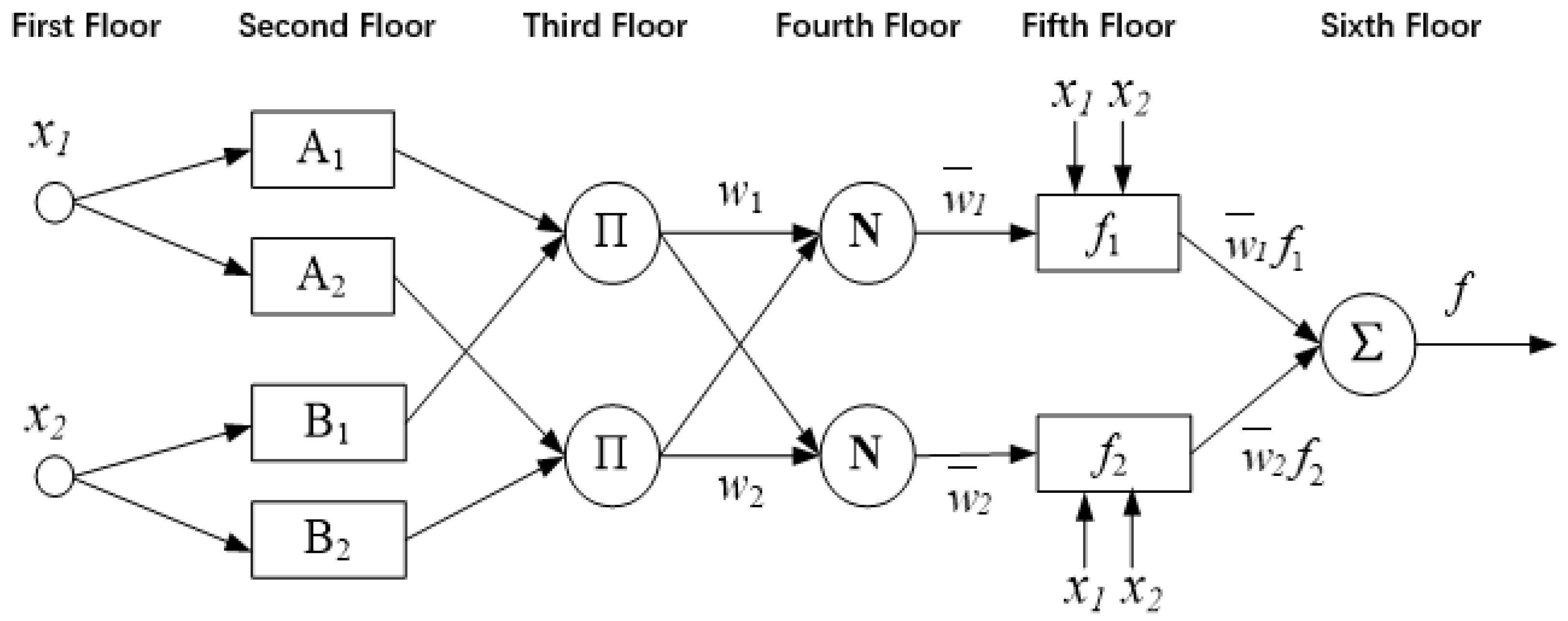The ANFIS leverages the strengths of both neural networks and fuzzy systems by encompassing neural network learning mechanisms and fuzzy system inference capabilities [25]. This makes the ANFIS a suitable choice for modeling and analyzing the dynamic risk assessment of traffic operations on typical road sections. The ANFIS was originally proposed to facilitate the analysis of key accident characteristics and provide effective accident prevention strategies. This ANFIS is equivalent to a first-order Sugeno fuzzy model. Through training and learning, the ANFIS can quickly and precisely calculate optimal parameters for membership functions, effectively simulating real input–output relationships. The ANFIS has many advantages, such as the ability to converge rapidly, the requirement for a small sample size, and the generation of limited error. The equivalent ANFIS structure of the Sugeno fuzzy system is shown in Figure 1.

In Figure 1, the connecting lines between nodes depict the flow of information, and square and circular nodes represent adjustable and non-adjustable parameters, respectively. The diagram reveals that only floors 2 and 5 contain adjustable parameters. Nodes on the same floor share identical functions. With the input of the i_th node in the kth floor denoted as O_ik, the functions of each floor within the ANFIS structure are as follows [25]:

• Floor 1: Input floor. The purpose of this floor is to transmit unaltered input variables to the next floor. Thus, the node’s output can be represented as follows:

$$O_i^1=x_i$$

(1)

2.

Floor 2: Fuzzification floor. The role of this floor is to generate fuzzy input variables to generate the corresponding membership function. Each unit on this floor signifies a segmented fuzzy subset. The transfer function of a node can be expressed as follows:

$$O_i^2={\mu }_{A_i}\left(x_1\right)$$

(2)

where $x_1$ is the input to the node, $A_i$ is the linguistic variable associated with that node’s function (e.g., high, low), and $O_i^1$ is the membership function of $A_i$, which indicates how well $x_1$ satisfies $A_i$. Normally, ${\mu }_{A_i}\left(x_1\right)$ can be either a bell-shaped membership or a Gaussian membership function expressed as follows:

$${\mu }_{A_i}\left(x_1\right)=\frac{1}{1+{\left[\frac{(x_1-c_i)}{a_i}\right]}^{b_i}}$$

(3)

$${\mu }_{A_i}\left(x_1\right)=\exp \left[\frac{-{(x_1-c_i)}^2}{{a_i}^2}\right]$$

(4)

where $\{a_i,b_i,c_i\}$ is the set of parameters for the floor. These parameters are referred to as premise or condition parameters.

3.

Floor 3: Fuzzy operation floor. This floor executes fuzzy set operations under certain conditions, combining various fuzzy subsets of different variables to create corresponding rules. The output represents the degree of applicability of each rule, typically calculated by the following equation:

$$O_i^3=w_i={\mu }_{A_i}\left(x_1\right)\times {\mu }_{B_i}\left(x_2\right)$$

(5)

Each node’s output indicates the incentive strength of the corresponding rule.

4.

Floor 4: Normalization floor. This floor normalizes the applicability of each rule. The normalized incentive strength of rule i is calculated by dividing the incentive strength of that rule by the sum of incentive strengths across all rules as follows:

$$O_i^4=\overline{w_i}=\frac{w_i}{w_1+w_2}$$

(6)

5.

Floor 5: Conclusion floor. This floor computes the output of each rule. The transfer functions of nodes in this floor are linear functions, with inputs consisting of network input and normalized incentive strength transmitted by floor 3. Node outputs are obtained by multiplying the transfer function with the normalized incentive strength as follows:

$$O_i^5=\overline{w_i}\times f_i=\overline{w_i}\times (m_i{x}_1+m_i{x}_2+l_i)$$

(7)

where $\{m_i,n_i,l_i\}$ is the set of parameters for the floor. These parameters are referred to as conclusion parameters.

6.

Floor 6: Output floor. This floor calculates the output of the fuzzy system, which is represented as the sum of the outputs of all rules as follows:

$$O_i^6=f=\sum \overline{w_i}{f}_i=\frac{\sum _i{w}_i{f}_i}{\sum _i{w}_i}$$

(8)

The main purpose of the ANFIS system is to employ a neural network learning mechanism to adjust the structure and parameters of the fuzzy system. Structural adjustments involve modifying the number of variables and domain division, whereas parameter adjustments concern parameters associated with membership functions, such as center and slope. When the network structure is established, ANFIS learning involves only parameter tuning. According to the literature, four main methods are used for parameter tuning. This study employs a hybrid learning algorithm consisting of gradient descent and least squares methods to adjust all parameters of the ANFIS. The advantages of the ANFIS hybrid learning algorithm include its optimization of conclusion rule parameters using the least squares method under fixed conditional parameters. In terms of operational speed, the hybrid learning algorithm outperforms gradient descent when used alone.

2.2. Decision Tree Analysis

The decision tree method is straightforward, intuitive, easy to verify, and highly efficient. A decision tree is a data analysis technique that has emerged from the fields of machine learning and data mining. It primarily employs recursive partitioning to predict and segment data. The resulting model from the decision tree method is represented as a hierarchical tree structure. Given their proficiency in handling non-numerical data and the clarity of their outcomes, decision trees have found wide-ranging applications across various domains. In the realm of transportation, decision trees have also been extensively used. Examples include the use of decision trees in studying vehicle actions (start/stop) when under a yellow light [26], analyzing parameters that affect traffic accidents, researching driver self-feedback mechanisms, and investigating key parameters in assessing the quality of transportation system services. This study integrates the decision tree approach into the dynamic risk assessment and modeling of traffic operations in typical road sections.

Decision trees achieve data classification through a series of rules. A decision tree has a tree-like structure composed of root nodes, subnodes, and branches. Roots and subnodes represent the entire dataset and individual variables, respectively. Connections between roots and subnodes are established through branches. When a node cannot be further divided, it becomes a terminal node, representing a final set of variables; otherwise, it is referred to as an internal node. The tree structure of a decision tree can be envisioned as the sequential execution of a series of decision rules. Each decision rule constitutes a branch of the decision tree, linking the root nodes to the terminal nodes.

A decision tree is constructed in two steps. In the first step, an initial split is determined to identify the optimal attribute domain for classification. The second step involves establishing decision tree branches based on distinct values of recorded fields. The difficulty of the decision tree algorithm is in selecting suitable branch values. The quality of branch values not only affects the growth rate of the decision tree but significantly affects its structure.

Currently, three primary classification algorithms are used for decision trees: iterative dichotomies, classification and regression trees (CART), and supervised learning. The CART algorithm can prevent excessive pruning of the decision tree and automatically prune the tree to its smallest size. In addition, the resulting tree structure can be evaluated using cross-validation. Thus, this study employs the CART algorithm for decision tree analysis.

Assuming X and Y are input and output variables, respectively, and Y is a continuous variable, given a training dataset of D = {(x₁, y₁), (x₂, y₂), …, (x_N, y_N)}, where x_i = (x_i⁽¹⁾, x_i⁽²⁾, …, x_i⁽ⁿ⁾) is the input instance (feature vector), n is the number of features, and i = 1, 2, N, where N is the sample size. We use heuristic methods to partition the feature space, examining all the values of all features in the current set one by one during each partition and selecting the optimal one as the segmentation point based on the minimum squared error criterion. For the j-th feature variable x_j and its value s in the training set, as the segmentation variable and segmentation point, and defining two regions R₁(s, j) = {x|x^(j) < s} and R₂(s, j) = {x|x^(j) > s}, to find the optimal j and s, solve the following equation:

$${min}_{j,s}[{min}_{c_1}\sum _{x_i\in R_1(j,s)}{(y_i-c_1)}^2+{min}_{c_2}\sum _{x_i\in R_2(j,s)}{(y_i-c_2)}^2]$$

(9)

That is, to find the j and s that minimize the sum of squared errors between the two regions to be divided. Among them, c₁ and c₂ are fixed output values in the two regions after division, and these two optimal output values are the mean of Y in their respective regions. Therefore, the above equation can be written as:

$${min}_{j,s}[{\sum }_{x_i\in R_1(j,s)}{(y_i-\widehat{c_1})}^2+{\sum }_{x_i\in R_2(j,s)}{(y_i-\widehat{c_2})}^2]$$

(10)

Here, $\widehat{c_1}=\frac{1}{N_1}\sum _{x_i\in R_1(j,s)}{y}_i$, $\widehat{c_2}=\frac{1}{N_2}\sum _{x_i\in R_2(j,s)}{y}_i$.

3. Data Acquisition and Experimental Setup

The dynamic risk of highway traffic operation is influenced by various factors, including road alignment, weather, traffic flow operation, and driver behavior. These factors interact with each other and, together, affect the dynamic risk level of transportation operations. In practice, it is impossible to investigate and collect all factors separately. Given the difficulty in obtaining information related to immediate changes in weather, road alignment, and driver behavior, coupled with changes in traffic flow and accidents, it best represents the dynamic risk state of road traffic operations. This study focuses on collecting traffic flow data and accident information captured by microwave coils and videos for modeling and analysis of dynamic risk assessment in traffic operations. Accident data includes detailed information such as time, location, type, and cause. The traffic flow data includes parameters such as speed, flow, and occupancy rate for each 30 s detection cycle of dividing lanes.

To obtain an accurate analysis of the characteristics of dynamic risk changes in traffic operations and to explore the relationship between dynamic risk and traffic accidents, traffic flow and accident data must be screened and processed. Crash and traffic flow data derived from external factors such as weather, road alignment, and individual driver behavior were excluded from the data cases whenever possible. In addition, because the relationship between single-vehicle accidents and traffic operations is not strong at high service levels, accident samples were selected with a preference for multi-vehicle accidents occurring at higher traffic volumes (i.e., below the level of Service C according to the HCM2010 [27]). To enhance data analysis accuracy and reliability, this study also conducted calibration and processing of traffic flow data. This involved identifying outliers using spatio-temporal graph methods and statistical techniques, while correcting outliers using linear interpolation and filtering. This enabled us to select detector data of better quality for traffic flow parameters such as time mean speed, coefficient of variation of speed, flow rate, and occupancy. Suitable cases for modeling and validation analysis of dynamic risk assessment for traffic operations could then be selected by matching detector data with accident data.

As previously mentioned, this study mainly leveraged traffic flow data and accident data to assess the dynamic risks of traffic operations. The studied road segment was the Beijing section of the Beijing–Harbin Expressway, which has a length of approximately 39.7 km. The study deployed 20 microwave detectors to detect traffic flow data in both directions and 16 video vehicle detectors to detect data in a single direction.

Given that traffic police tend to record only the cross-section stake information when noting accident locations, the traffic flow data of the respective cross-sections was chosen as the primary parameter for analyzing the relationship between traffic flow and accident generation. The following data conversion formulas for transforming divided-lane traffic flow data into cross-sectional traffic flow data were applied.

$$q_s={\displaystyle \sum _{i=1}^n{q}_i}$$

(11)

$$k_s=\frac{{\displaystyle \sum _{i=1}^n{q}_i\cdot k_i}}{{\displaystyle \sum _{i=1}^n{q}_i}}$$

(12)

$$v_s=\frac{{\displaystyle \sum _{i=1}^n{q}_i\cdot v_i}}{{\displaystyle \sum _{i=1}^n{q}_i}}$$

(13)

where $q_i$, $k_i$, and $v_i$ are the traffic volume, occupancy, and speed of the divided lane, respectively, and $n$ is the total number of lanes.

For dynamic risk assessment, another important issue is identifying the right periods and intervals for data collection and modeling analysis. Referring to relevant literature, this study used traffic flow data for each traffic accident derived from the upstream detector section at every 10-min interval within a 30-min period prior to the accident’s occurrence. The study also used traffic flow data for the respective accident control groups. The selection criteria for the control group were as follows: (1) the control group’s date differs from the corresponding accident date; (2) the control group’s date coincides with the accident’s occurrence time; (3) the control group’s date matches the location of the accident; and (4) the control group’s date corresponds to a day when no accidents occurred at that location. In addition, to mitigate the potential impact of different traffic characteristics on weekends and weekdays on the risk assessment model, as the control group, this study independently chose traffic flow data from the same 30-min period of the upstream detector section on the seventh and 14th days prior to the accident. By aligning detector data with accident records, this study ultimately selected 123 samples with accident data and 246 samples from the control group without accident occurrences. The samples were used for dynamic analysis, modeling evaluation, and validation analysis. The collected traffic flow parameters are listed in

Table 1. Cross-section traffic flow parameters.

Parameter	Unit	Variable
Average value of cross-section flow	veh/30 s	Qavg
Standard deviation of cross-section flow	veh/30 s	Qsd
Coefficient of variation of cross-section flow	%	Qcsv
Average value of cross-section speed	km/h	Vavg
Standard deviation of cross-section speed	km/h	Vsd
Coefficient of variation of cross-section speed	%	Vcsv
Average value of cross-section occupancy	%	Oavg
Standard deviation of cross-section occupancy	%	Osd
Coefficient of variation of cross-section occupancy	%	Ocsv

.

4. Results and Discussion

This section presents the results derived from our study based on the integrated modeling method, decision tree, and ANFIS.

4.1. Modeling Method

The approach involves using decision trees to identify the primary influencing factors on dynamic risk in traffic operations and then utilizing these factors for dynamic risk assessment modeling. Based on the modeling results of decision trees, the key factors affecting dynamic risk can be determined under different data collection periods. These factors can then serve as input parameters, with the defined dynamic risk values used as output parameters for the ANFIS dynamic risk assessment model.

To achieve an accurate analysis of the effects and differences of various dynamic risk assessment models, the same training and evaluation samples should be chosen for data modeling. The definitions of dynamic risk values should also remain consistent. In other words, for decision tree risk assessment modeling based on 5-min data, the dynamic risk values are defined as follows: For the accident group, the risk values are all given as 1 in the 5 min preceding the accident. For the accident-free control group, their risk values are relatively low, remaining at 0 in the first 5 min. As with the ANFIS modeling approach, the same 103 accident groups and their corresponding 206 control groups with upstream detector cross-section data over a 5-min period were selected as training samples. In addition, the 20 accident groups and their corresponding 40 controls with upstream detector cross-section data over a 5-min period were used as evaluation samples. And the results of the decision tree based on the 5-min and 10-min data can be found in the Figure 1 and Figure 2.

Furthermore, based on the aforementioned modeling approach, the saved rules could be employed to predict the dynamic risk values in the evaluation samples, enabling the analysis of model errors.

Similarly, with the same training and evaluation samples as used under the ANFIS method and based on the dynamic value-at-risk definitions in both the ANFIS and previously described decision tree modeling approaches, decision tree results for the 10-min, 20-min, and 30-min data collection durations were derived (see Figure 3, Figure 4 and Figure 5). Overall, the decision tree algorithm has achieved good results. In the final obtained node, IM < 0.05 (see Figure 2, Figure 3, Figure 4 and Figure 5) indicates good classification performance of the node.

According to the results of the decision tree, the influencing factors on dynamic risk under a 10-min data collection duration were Q_avg (average value of cross-section flow), Q_sd, O_avg, O_sd (standard deviation of cross-section occupancy), and O_csv (coefficient of variation of cross-section occupancy). We will use this dimension to model the risk in Section 4.2.

Different from the modeling of the 5-min data and 10-min data, the key factors of the 20-min data included Qavg, Qsd, Qcsv, Vavg, Vcsv (coefficient of variation of cross-section speed), Oavg, and Osd (see Table 1 for a list of all parameter definitions). These parameters were taken as inputs to the model in the modeling of scenarios after 20 min. And the main influencing factors of dynamic risk, as depicted in Figure 5, were Q_avg, Q_sd, Q_csv, V_avg, O_avg, O_sd, and O_csv, which will be set as the inputs in the risk modeling based on 30-min data.

4.2. Integrated Modeling Results Based on Decision Trees and ANFIS

The node information presented in Figure 2 reveals that the main influencing factors of dynamic risk under a 5-min data collection period were F_sd (standard deviation of cross-section flow), Q_csv (coefficient of variation of cross-section flow), Vavg (average value of cross-section speed), V_sd (standard deviation of cross-section speed), and O_avg (average value of cross-section occupancy) (see Table 1 for a list of all parameter definitions). Accordingly, these were selected as the model input parameters. The output parameters consisted of the traffic operation risk values in the first 5 min for both the accident and control groups. Given that risk values increase when an accident is about to occur, the risk values for the accident group were higher in the first 5 min prior to the accident (all were equal to 1). By contrast, in the control group, in which no accidents occurred, lower risk values were exhibited during the same period (all were equal to 0).

In this study, the aforementioned 103 accident groups and their corresponding 206 control groups were selected as training samples, and 20 accident groups and their corresponding 40 control groups were chosen as evaluation samples. The resulting input–output data curves for the risk assessment model based on a 5-min data collection period are presented in Figure 6 and Figure 7.

In Figure 6, the x axis is the time before the scenario of assessment. For example, when time is 150 s, it refers to the situation that occurred 150 s before the scenario. We use the traffic flow characteristics that 150 s advance to assess the risk of the expressways. To better quantify the risk of the expressway with the operation data, the decision trees and ANFIS under different time intervals have also been discussed. The node information presented in Figure 3 reveals that the primary influencing factors on dynamic risk under a 10-min data collection duration were Q_avg (average value of cross-section flow), Q_sd, O_avg, O_sd (standard deviation of cross-section occupancy), and O_csv (coefficient of variation of cross-section occupancy) (see Table 1 for a list of all parameter definitions). At about time = 15 s, the traffic flow is stable, and the value of the volume and the standard deviation of velocity are relatively low, which means the scenario is very safe (risky value < 0, safer than the norm scenario). At about time = 150 s, it can be found that the value of occupancy rapidly increased and the mean velocity decreased to nearly 0 m/s. This is because of a jam caused by the accident. In this scenario, our method gives a higher risk value (nearly 1.0), which indicates our method can capture the transition of road safety effectively.

Based on the data of the aforementioned main factors of the upstream detector cross section of the accident group for the 10-min period prior to accident occurrence and the corresponding data of the control group, these parameters were imported into the model. This enabled ANFIS-based dynamic risk assessment to be modeled. In addition, the output parameter set represented traffic operation risk values at 10-min intervals for both the accident and control groups. At this juncture, it could be posited that risk values increased as the accident moment approached and decreased as the accident moment passed. Within the 10-min period prior to the accident, risk values showed a linear increment. For the accident group, the risk value during the first 5-min interval prior to the accident was defined as 1, whereas that during the 5- to 10-min interval prior to the accident was defined as 0. By contrast, the control group’s risk values remained at 0 for all intervals. Based on the same training and evaluation samples, Figure 8 and Figure 9 display the input–output data curves of the dynamic risk assessment model based on 10-min data and the training step-error curves of the model, respectively. The figures show that the errors were reduced as compared with the results based on 5-min data (see Figure 7 and Figure 9 and

Table 2. Dynamic risk assessment model errors for different data periods.

Method	Error	Duration
		5 min	10 min	15 min	20 min	25 min	30 min
Decision Trees and ANFIS	Training error	0.448	0.361	0.322	0.310	0.303	0.280
	Evaluation error	0.469	0.392	0.347	0.328	0.317	0.289

).

Similarly, the risk assessment with 20-min and 30-min data have been conducted. The main influencing factors of dynamic risk under a 20-min data collection period, as shown in Figure 4, included Q_avg, Q_sd, Q_csv, V_avg, V_csv (coefficient of variation of cross-section speed), O_avg, and O_sd (see Table 1 for a list of all parameter definitions). These parameters were taken as inputs to the model, with the output parameters representing traffic operation risk values at 5-min intervals for both the accident and control groups. Similar to the previous case, risk values were presumed to increase linearly from 20 min prior to the accident up to the accident moment. For the accident group, the risk value during the first 5-min interval before the accident was defined as 1, and then the values for the second through fourth intervals were set to 2/3, 1/3, and 0, respectively. By contrast, the control group risk values remained at 0 for all intervals. Under the 30-min data collection duration, the main influencing factors of dynamic risk as depicted in Figure 5 were Q_avg, Q_sd, Q_csv, V_avg, O_avg, O_sd, and O_csv (see Table 1 for a list of all parameter definitions). These factors were used as inputs to the model, whereas the output parameters represented traffic operation risk values at 5-min intervals for both the accident and control groups. Likewise, the risk values were assumed to increase linearly from 30 min prior to the accident to the accident moment. For the accident group, the risk value during the first 5-min interval prior to the accident was defined as 1. The risk values for the second through sixth intervals were set to 0.8, 0.6, 0.4, 0.2, and 0, respectively. By contrast, the control group risk values remained at 0 for all intervals.

Figure 10 and Figure 11 show the model results obtained using the same training and evaluation samples with 20-min data. The model results obtained using the same training and evaluation samples with 30-min data are presented in Figure 12 and Figure 13. The comprehensive modeling results when combining decision trees and the ANFIS revealed that the risk values observed 30 min prior to the accident aligned closely with the predicted values. The model results provide insights into the errors of the dynamic risk assessment model based on different data periods, as shown in Figure 14.

Table 2 reveals that the lowest model errors, namely, 0.280 and 0.289 for the training and evaluation samples, respectively, were obtained by employing dynamic risk assessment modeling under decision trees and ANFIS. These were based on data from the upstream detector cross sections taken during the 30 min prior to the accident for the accident group and corresponding control group. Figure 14 shows the dynamic risk predictions and observations for the evaluation samples at this stage.

Figure 14 shows that a predicted dynamic risk value of greater than 0.6 typically accompanied an accident occurrence. Therefore, an accident prediction threshold of 0.6 could be established, where a risk value surpassing this threshold signifies an impending accident. For the selected 150 evaluation samples with accidents, using 0.6 as the prediction threshold resulted in 116 predicted accidents, yielding a forecasting accuracy of 77.3%. By contrast, of the 300 evaluation samples without accidents, only 17 were wrongly predicted as accidents, resulting in a false alarm rate of merely 5.7%. The modeling and results could be applied to real-time traffic operational risk monitoring to facilitate the prediction of road accidents.

Under dynamic risk assessment, a detected risk value of greater than 0.6 suggests the likelihood of an accident. In these instances, implementing dynamic traffic control measures can effectively prevent or mitigate accidents.

Based on the decision tree analysis presented in Figure 5, the main influencing factors of dynamic traffic operation risk under the 30-min data collection duration included Q_avg, Q_sd, Q_csv, V_avg, O_avg, O_sd, and O_csv (see Table 1 for a list of all parameter definitions). These underscore the fact that implementing appropriate control measures for flow, speed, and occupancy can reduce the likelihood of accidents.

5. Conclusions

This study established a technological system for dynamic risk assessment on expressways based on the Beijing–Harbin Expressway, used as a representative road section in China. The system consists of finely grained models that operate on a minute-level dimension. For periods in which accidents are of high risk, a fine-grained risk assessment is performed at the minute level. Following analysis of accident and traffic flow data, input parameters for the dynamic risk assessment model were derived. Data within the 5-, 10-, 20-, and 30-min periods prior to the occurrence of accidents were used to determine suitable data collection and model-training time frames, define risk values, and conduct dynamic risk assessment modeling. Error analysis showed that selecting data from the first 30 min prior to the occurrence of accidents as well as data from the first 30 min of the corresponding control group for the dynamic risk assessment modeling based on decision trees and ANFIS resulted in the smallest model errors and a high accuracy in accident prediction. Specifically, decision trees were employed to identify the primary influencing factors of dynamic traffic operation risk, and these were then used for ANFIS modeling. Therefore, for the dynamic risk assessment of traffic operations on an expressway section in an urban agglomeration, employing data from the 30 min prior to accidents for training and simulation of a dynamic risk assessment model is recommended. The trained model can be used for a real-time assessment of traffic operation risk within each time interval. Effective control measures such as the issuance of risk warnings, accident forecasts, lane management, and speed control can be employed if risk values are greater than 0.6.

Overall, this study shifted the focus from ex-post risk evaluation to ex-ante risk analysis. This marks a departure from the traditional approach of relying solely on statistical and historical data for road risk analysis. The findings can be applied to real-time monitoring of traffic operation risk levels on roads and serve as the basis for developing targeted accident alerts and traffic control measures. This approach enhances the technology and efficiency of traffic safety management to ensure road traffic safety. The main significance of this study is reflected in the following aspects:

(1) For a certain scenario, we can conduct safety assessments in advance based on its traffic flow characteristic data, transforming post-evaluation into pre-evaluation.

(2) This study used data from China and focused on expressions in urban agglomerations. It can be directly applied to expressions in Chinese agglomerations, filling the gap in related fields.

In this article, we mainly considered the characteristics of traffic flow and conducted a dynamic risk assessment model. However, this study still has the following shortcomings:

Firstly, we only considered some relatively simple traffic flow characteristics. In order to better model, some complex features should also be considered, such as the distribution of speeds on different lanes and the correlation coefficient between the speeds of front and rear vehicles [19].

Secondly, we did not consider static risk assessment factors [28] and environmental characteristics (such as weather characteristics [29]). Considering that traffic safety is a complex system, incomplete feature inputs may introduce heterogeneity and bias [21].

Our further research will be focused on assessment models with more comprehensive factors. Through intelligent description and factor analysis of a large amount of traffic flow data, traffic environment, road facilities, and traffic accident data, we will extract indicator parameters that can reflect the dynamic and static risk levels of road traffic safety, further eliminate heterogeneity, and provide a more reliable model for the safety assessment of Chinese expressways.