Abstract
In rural areas of China, the challenges of efficient and cost-effective distribution are exacerbated by underdeveloped infrastructure and low population density, with last mile logistics distribution posing a significant obstacle. To address the gap in drone application for last mile logistics in rural areas, a truck–drone distribution model was developed based on the specific conditions of rural regions. The improved fuzzy C-means algorithm (FCM) and genetic simulated annealing algorithm (GASA) were employed to tackle real−world cases in rural areas. The focus of the truck–drone system is to optimize the rural logistics distribution process, reduce delivery time, and minimize costs while considering factors such as maximum mileage of trucks and drones as well as customer priority. Compared to traditional methods, this system has demonstrated notable improvements in distribution efficiency and cost reduction, offering valuable insights for practical drone applications in last mile rural logistics.
1. Introduction
With the revitalization of rural areas and the improvement in rural consumption and living standards, the online purchasing power of rural customers is growing stronger and stronger. A report [1] indicates that the online retail sales in rural areas of China surged from 0.18 trillion yuan(CNY) in 2014 to 2.17 trillion yuan in 2022, with over 300 million internet users in rural areas. Additionally, the online retail sales of agricultural products reached 0.53 trillion yuan, marking a year−on−year increase of 9.2%. However, unlike cities with better logistics capabilities, rural logistics often have problems such as low distribution efficiency and the need to pick up goods over long distances [2,3]. There are three major transportation difficulties in the “last mile” of rural logistics distribution:
- (1)
- The transportation distance is long, and customers are scattered in rural areas with vast terrain. The sparse distribution of customers not only leads to longer transportation distances and more difficult logistics distribution but also requires logistics companies to formulate more complex and flexible strategies in resource planning and route optimization.
- (2)
- Complex geographical environments and poor road conditions. The rural geographical environment is complex, the terrain is undulating, the mountain roads are rugged, and road conditions are often poor across rivers, which also affects the speed and safety of rural cargo transportation.
- (3)
- Shortage of human resources. There is a shortage of human resources in rural areas and a lack of professional logistics personnel, making it difficult to ensure the quality and efficiency of logistics.
The emergence of drones as a new mode of transportation will significantly drive the advancement of the transportation logistics industry, and it also serves as an effective solution to the last mile transportation challenge in rural areas. Drones have the advantages of not being restricted by ground transportation, reducing high labor costs, environmental protection, and saving energy. Products that need cold chain transportation technology, such as specialty fresh foods and medical supplies, or goods that cannot be transported due to distance problems, can be delivered to customers more quickly through the use of drones [4]. It is possible to completely change the traditional way of parcel delivery by using drones. Because drones can fly over obstacles on the ground, they can choose a more direct route and a shorter distance than traditional trucks. The package is delivered directly within the time limit [5], so the flight speed of drones is usually higher than that of traditional trucks [6]. Therefore, drone delivery can not only reduce costs, but also improve the speed of logistics in the last mile [7].
The logistics challenges associated with the use of drones have garnered significant attention. Over the past few years, there has been a rapid increase in the utilization of drones across various sectors, including real−time monitoring, wireless coverage provision, remote sensing, search and rescue operations, inspection activities, and goods transportation (Otto et al. 2018) [6]. In terms of the application of logistics and transportation of drones, in 2013, Amazon announced the idea of using drones to complete orders. Orders within its Prime Air delivery plan can be delivered to customers within 30 min through drones. In China, starting in 2016, JD company has been actively expanding the delivery services of drones, testing drones to serve customers in rural areas. Subsequently, Joseph Tokosh investigated whether Amazon distribution centers are suitable as potential drone launching facilities [8], and Abderahman Rejeb further reviewed 55 articles about drone logistics, and summarized the advantages and disadvantages of drone logistics [9].
In practical scenarios, drone logistics are subject to certain technical constraints, including limitations on payload capacity, battery life, and information security and safety, all of which require further enhancement. Therefore, Murray and Chu (2015) initially put forward a model [10] combining trucks and drones, which is called the “Flying Partner Traveling Salesman Problem” (FSTSP). This problem was inspired by the vehicle routing problem with synchronization constraints (Drexl, 2012) [11]. In the latest study of two−stage drone delivery, Aero designed a heuristic method based on mixed integer programs to solve the parallel delivery model of drones and transport vehicles [12], and Bipan Zou proposed a novel locker–drone delivery system, where trucks deliver packages from warehouses to lockers, and drones complete the final delivery [13]. They provide more feasible solutions for the application of drones in the logistics field.
Initially, the literature review reveals challenges in last mile logistics within rural areas, marked by inadequate road conditions and extended transportation distances, resulting in high logistics costs. As an emerging mode of transportation, drones demonstrate adept navigation through intricate rural landscapes, offering both cost efficiency and environmental sustainability. However, there are still challenges in achieving complete drone delivery. To address these issues, joint methods and solution algorithms of a truck–drone system were explored as a feasible combined transportation approach. Our main concern is the last mile delivery in rural areas, especially exploring the distance between truck and drone combined transportation.
Hence, the current situation of rural logistics distribution has been consolidated, with trucks serving as the focal point for drone distribution. Our emphasis lies in addressing the site path optimization challenge within the truck–drone logistics distribution framework. After the truck delivers the drone team to the designated village center, the drone team will pick up the packages and deliver them individually to the customers. After completing the delivery task, they will return to the distribution center collectively.
The innovation of this paper is to establish a mathematical model based on actual assumptions, and carefully consider the real scenarios with the goal of lowest cost and shortest customer waiting time. The model is designed to optimize the delivery process of the last mile and reduce the challenges faced in rural logistics. To verify the method, a two−stage path optimization algorithm has been implemented, combining the improved fuzzy C−means algorithm (FCM) and genetic simulated annealing algorithm (GASA). The MATLAB simulation utilized real data from a 1600 square kilometer area in rural China, providing empirical insights into the model and algorithm performance.
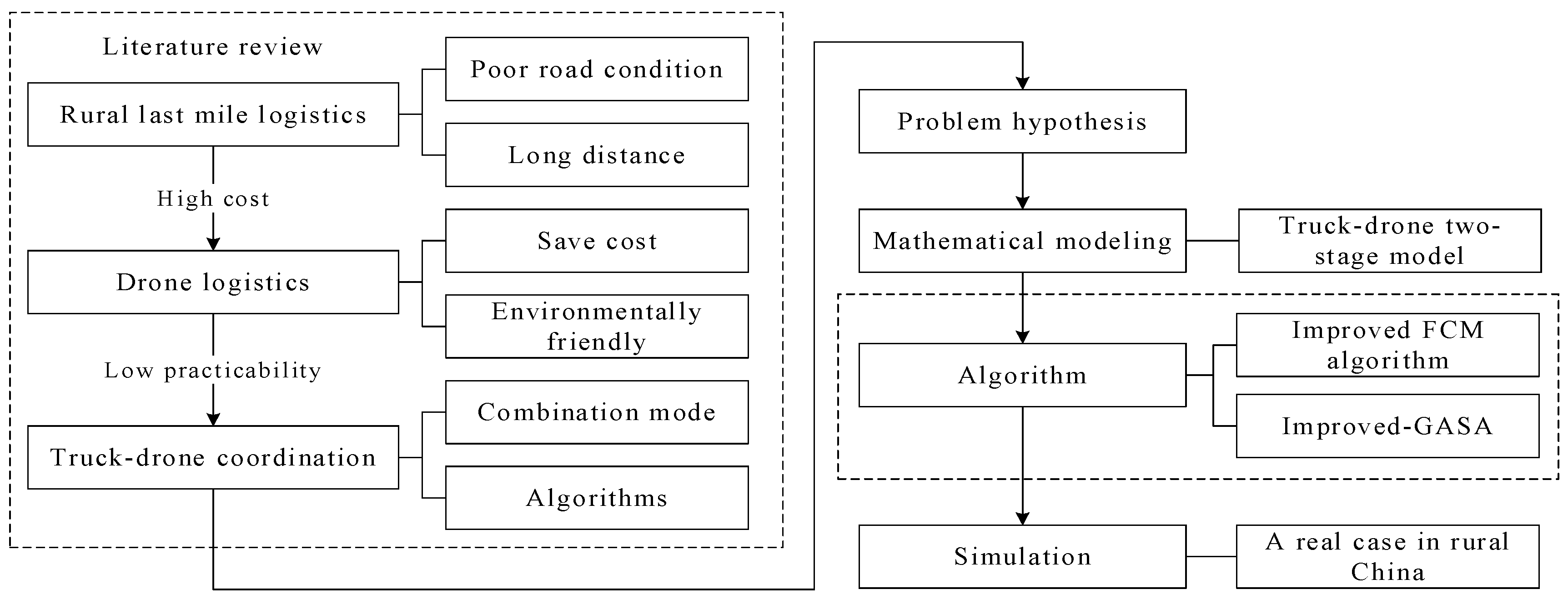
The research structure shown in Figure 1 summarizes the systematic method employed to address the complexities of last mile logistics in rural areas, offering a new perspective for integrating truck and drone transportation to enhance efficiency and reduce costs. The rest of the paper is organized as follows. Section 2 reviews the research literature on three key aspects: rural last mile, drone logistics, and truck–drone combined transportation. It highlights the current research shortcomings in these areas. Section 3 and Section 4 describe this problem in digital form and establish a mathematical model according to the distribution situation of the last mile in rural areas. Section 5 explains the two−stage path optimization algorithm used in this article. In Section 6, MATLAB simulations are conducted using real data from an area in rural China, and the experimental results are illustrated. Section 7 summarizes the main findings of the contribution and provides directions for future research.
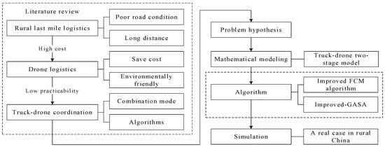
Figure 1.
Research framework.
2. Literature Review
In order to clarify the research status of the truck–drone transportation mode in the last mile logistics in rural areas, the literature review is divided into three main sections. The first section introduces different research documents about the last mile traffic in rural areas. Then, the related path planning literature of drones was reviewed, and the advantages and disadvantages of drone logistics applications were explained. The last section briefly reviews the literature related to truck–drone combined transportation, including related algorithms.
2.1. Rural Last Mile Logistics for Long Distance and High Cost
Logistics in rural areas of China has long been plagued by the challenges of extended transportation distances and high costs. In the context of utilizing drones for last mile delivery in remote or rural areas, PAN has raised the issue of selecting suitable logistics centers for drone operations. Employing a straightforward model that incorporates factors like village traffic and size, PAN applied a compact cuckoo search algorithm utilizing mixed uniform sampling technology to effectively address the problem [14]. In the role of cooperation in the last mile logistics in rural areas, Yang Fei used cooperative VRP games to study how three typical logistics providers cooperate to consider the significant differences between rural logistics environment and logistics value chain participants. The efficiency and effectiveness of the last mile logistics in rural areas have been improved [15]. Ivana Nikolić proposed an interval−type fuzzy AROMAN approach to consider the location and presence decisions of postal branches for implementation by policymakers and industry managers to optimize postal networks [16]. Despite the escalating demand for rural logistics, the traditional establishment of express delivery points demands substantial manpower and resources, failing to promptly address the existing supply–demand imbalance. There is an urgent need for innovation to solve the logistics challenges of the last mile in rural areas.
Currently, the customer pick−up process in the final mile of rural logistics is excessively lengthy, and any cost or carbon emissions saved from establishing self−pick−up points are negated during the customer self−pick−up process. For customers in rural areas with many elderly and children, the pick−up stations are far from their homes. It typically takes 3–4 days for rural customers to collect goods in the township, which is unfavorable for time−sensitive items like fresh food and medicines. Numerous scholars have also conducted research on enhancing logistics efficiency in rural areas, R. Niemeijer’s research found that in rural areas, the carbon emission benefits brought by self−pickup points to improve the efficiency of delivery routes will soon be offset by the carbon footprint related to customer travel [17], which is not conducive to reducing carbon emissions. Lalith Pankaj Raj Nadimuthu innovatively designed and carried out the experimental study of a thermoelectric micro−cold storage system driven by solar photovoltaics. This system serves as a COVID−19 vaccine carrier in rural areas, expediting vaccine delivery to remote regions while concurrently mitigating carbon emissions [18]. Yang Tiannuo introduced a demand−driven integrated passenger and freight service (DDPFIS) model, which uses a novel mixed integer linear programming method to solve the green vehicle routing problem. This model aids public transportation operators in intricate decision−making, resulting in reduced fuel consumption and costs. It is particularly applicable for serving time-insensitive rural residents [19]. For rural logistics customers, the convenience of returning goods, the integrity of goods, reservation for picking up goods and the distribution cost are the most basic factors that affect the sustainability of rural last mile distribution [20]. To optimize the last mile delivery cost in rural areas, Xiaofei Kou introduced a multimodal transportation design, incorporating three key transportation modes—local logistics providers, public transportation, and crowdsourcing logistics. This solution adopts a genetic algorithm (GA) to effectively solve the logistics challenges [21].
2.2. Drone Logistics Saves Costs and Energy
As previously mentioned, the use of drones as a viable delivery method has been extensively researched, particularly in rural areas. The optimization of route planning for efficient distribution has become a focal point in rural logistics research. In the path planning of drones, the goal is to consider the delivery distance or the shortest delivery time. For example, Dorling considers the multi−range delivery of drones and aims to minimize the cost of delivery waiting time [22]. Rabat aimed to minimize the delivery distance of drones and plan the delivery routes of drones for disaster relief areas [23]. Shao applied drones to long−distance delivery, taking into account the existence of drone charging stations and maintenance stations, and planning drone flight routes to minimize the drone flight distance and drone landings times [24]. Yuan aimed at the shortest delivery time and used genetic algorithms to solve the path planning problem of multi−package heterogeneous drones. When considering logistics and delivery time, it is more realistic that those who exceed the expected delivery time of customers will be punished [25]. In the study of vehicle path planning with time windows, Wang extended the vehicle path planning problem with time windows, studied the dual path planning problem of vehicles with time windows considering customized service times, and developed a multi−ant colony optimization algorithm to solve this problem [26]. Spliet studied a vehicle route planning problem (TWAVRP) based on the time window of travel time allocation, which can allocate time windows among customers’ demands, which can better reduce expected transportation costs [27].
However, Niamat Ullah Ibne Hossain used the Bayesian network method and found that economic factors have the greatest impact on the overall performance of drone logistics transportation, followed by functional performance and technical responsiveness [28]. Ha (2018) [29] minimized the operating costs associated with transportation costs and waiting times. Their compact MILP formula is similar to Murray and Chu’s (2015) [10], and is only applicable to substitute objective function.
Compared with traditional truck transportation mode, drones have the advantages of fast transportation speed, high flexibility, low carbon, and environmental protection in rural areas, but it also has the limitations of short transportation distance and battery capacity. Thomas Kirschstein pointed out that from an energy perspective, in most cases it is not worthwhile to switch to a drone−based parcel delivery system alone, and in rural settings, a drone−based parcel delivery system incurs an energy demand similar to a parcel delivery system using electric trucks, assuming moderate environmental conditions [30]. Aishwarya Raghunatha found that when transporting goods in rural areas, the emissions generated by large drones are lower than those of diesel trucks, and drones cannot compete with electric trucks, mainly because the energy requirements for taking off and landing of drones are higher. Notably, electric drones are more economically cost−effective than road transport modes such as diesel and electric trucks but provide the fastest delivery times [31]. Using real−world delivery demand data, Elsayed simulated the drone and ground delivery modes of all−day parcel delivery services in urban and rural areas, and found that compared to the emissions generated by ground transportation, the emissions generated by drones were significantly reduced, and compared with those generated by electric vehicles, the emissions increased by 35% [32]. These studies demonstrate the feasibility of utilizing drones for logistics in rural areas. However, considering the issue of carbon emissions, simple drone delivery is not as effective as using electric vehicles for transporting goods. Therefore, an alternative approach would be to employ a combination of truck and drone transportation.
2.3. Truck–Drone Coordinated Operations and Algorithms
In the two−stage distribution research, Sung woo Kim proposed a solution to the coordination problem between drones and trucks by dividing the traveling salesman problem model of drone stations into independent traveling salesman and parallel identical machine scheduling problems. This approach aims to overcome the flight range limitations of the truck–drone system [33]. Enthoven studied a covered two−level vehicle route planning problem, dividing traditional transfer stations into two categories: lockers for customers to pick up goods themselves, and transfer stations for second−level vehicle transfers, through an iteration of the domain search algorithm. This process adds an adaptive searching process to solve this problem [34]. The multi−modal transport between drones and trucks is also considered as one of the effective methods to solve the last mile distribution problem in rural areas [20,35,36]. Aiming at the challenge of single truck and multi−drone delivery, Moshref−Javadi proposed a MILP model (2020) to minimize the waiting times for customers [37]. On the contrary, Kitjacharo−enchai (2019) introduced the MTSP−D, which allows a drone to autonomously execute parcel delivery by taking off from a truck, completing the delivery, and returning to any available truck nearby, regardless of capacity limitations [38]. In their study on a more efficient truck–drone package delivery system, Wang and others (2019) introduced a hybrid algorithm and utilized trucks, truck−mounted drones, and independent drones to optimize the entire delivery process [39].
For the shortest time target, YANPIRAT focuses on minimizing the total service time in order to reduce the final delivery time for trucks reaching the warehouse. Based on the meta−heuristic algorithm of variable neighborhood search, a method of joint operation between truck and drone is proposed. The new model integrates both delivery and returns, and is called the multi−cargo traveling salesman problem with integrated delivery and returns [40]. Zhou studied the two−layer vehicle routing problem with time window constraints and solved the problem of simultaneous delivery of goods. With the goal of minimizing total transportation mileage and maximizing customer satisfaction, Zhou proposed a variable neighborhood tabu search algorithm to solve this problem. Large−scale calculation examples have proved its strong adaptability [41]. Mohamed Salama developed a heuristic based on unsupervised machine learning using a joint optimization method to solve the problem of high computational cost when selecting cluster locations that are not fixed when multiple drones operating in conjunction with a single truck deliver orders to a group of customer locations. The algorithm speeds up the solving time [42]. In order to minimize the total cost, Alexander Rave used a special adaptive large neighborhood search to study the cost of trucks and drones under different coordination conditions. The results showed that launching drones from trucks and dedicated drone stations saves the most costs [43].
In the domain of logistics distribution algorithms, Karakatič conducted an off−science comparison among various genetic methods and alternative research approaches on the multi−site vehicle route standard benchmark problem. In this study, the popular crossover, mutation, and selection methods within genetic algorithms are comprehensively summarized and implemented. Subsequent tests have determined the most effective genetic operators, revealing the applicability of genetic algorithms in solving large NP problems, which exceed the exact algorithms and some heuristic methods [44]. Prajapati proposed a mixed integer nonlinear programming (MINLP) model, which took into account the costs caused by transportation, carbon tax, delay in delivery, and delivery in the first and last mile. Solving real−world scenario problems with four nature−inspired algorithms, the Firefly algorithm was found to provide the best optimal cost with Neighborhood Attractiveness, advanced particle swarm optimization algorithms can calculate the optimal cost in less computation time [45]. Ha (2020) proposed a hybrid algorithm combining a genetic algorithm and local search, and a single drone was used to solve the dual−objective TSP−D [46]. Sacramento et al. (2019) developed an ALNS to solve a VRPD with one drone per truck [47]; one particular limitation of the problems they considered was that the drones could not return to the same node as when they were launched, but had to return to a node that the truck would visit later on its route. Euchi and Sadok (2021) [48] formulated a hybrid genetic algorithm for a similar problem context, identifying multiple solutions that outperform the best−known solutions provided by Sacramento. Yang Wang [49] proposed a hybrid graph network model for the TSPD that is based on the DRL mechanism. The model has better generalization ability compared with the current DRL models.
The genetic algorithm is a widely utilized heuristic approach for addressing the path planning issue in drone operations. Xueli Wu et al. [50] and Zhenwen Zhou et al. [51] used immune genetic algorithms to study collaborative target search strategies for multi−UAV closed trajectories. Yi Tan et al. [52] used a genetic algorithm to solve the overlay path planning problem in the automatic detection of building surfaces. Ferranders (2016) used a genetic algorithm to solve the route of the truck, and used the K−means algorithm to solve the route of the drone according to the route of the truck [53]. Chang and Lee (2018) [54] enhanced their methodology by applying the classical TSP model to determine the shortest truck route that covers all cluster stops. However, as far as the last mile logistics in rural areas is concerned, the application of a genetic algorithm in the combined transportation of drones and trucks still needs further study.
The literature review above reveals that there is still a scarcity of research on the drone multi−stage delivery problem in the last mile drone path planning in rural areas. In the existing research, there are the following problems: first, the delivery cannot reach the customer directly. Deliveries are usually delivered directly to townships and customers need to pick up the goods far away from home. This is very inconvenient for the customers in rural areas with many elderly people and children, and there is a lack of effective solutions to deliver directly to customers. Secondly, the optimization objective is single. Currently, the majority of research focuses on optimizing either delivery time or delivery distance and lacks the dual consideration of both delivery costs and customer delivery time constraints. In addition, the urgency of delivery has been simplified, and all goods have been delivered by the same class. In practical problems, different customers and different products have different delivery urgencies and need to be treated differently. Thirdly, in order to solve the problem of drone distribution, most of the papers focused on the establishment and analysis of models, and the application of heuristic algorithms in drone logistics methods is not explored enough. The widely employed genetic algorithm has limited application in the context of truck–drone systems, warranting exploration in combined transportation scenarios.
To address these challenges, a drone−truck distribution model is developed, taking into consideration the specific features of rural logistics. The model aims to minimize customer waiting time and delivery cost simultaneously. At the same time, different levels of distribution priorities were established to achieve differentiated distribution. Although various optimization methods have been explored, such as genetic algorithms, mixed integer nonlinear programming (MINLP) models and hybrid methods, the complex nature of the last mile logistics in a rural environment requires more nuanced solution. The choice to employ the improved FCM algorithm and GASA algorithm in case simulations is grounded in the unique challenges identified in existing studies. Finally, an actual rural case is used to solve the problem, which verified the effectiveness of the model and algorithm.
3. Research Problem Description
At present, there is a three−level relationship between township, village, and customer in e−commerce logistics distribution in most rural areas in China. According to data from the State Post Bureau, the coverage rate of express township outlets is projected to reach 98% in 2020, with half of them capable of serving villages and only a small portion able to directly deliver to customers, indicating a significant disparity from the logistics standards of urban e−commerce. In the complex rural setting, distribution efficiency remains low while distribution costs remain high. Therefore, the scenario of using drones to deliver goods directly to customers is considered. The distribution system strives to deliver goods to customers within the expected time window, aiming at minimizing the costs and shortening the time. This strategic approach effectively enhances the efficiency of last mile distribution, ultimately reducing logistics expenses.
The specific two−stage transportation and distribution method can be divided into two stages. In the initial stage, taking into account the actual distribution of villages, multiple villages are considered as a cluster. Trucks departing from the township distribution center sequentially travel to each cluster center with packages and drones before returning to the township distribution center. The second stage involves the truck halting at the village gathering center, where the drone is deployed to commence its delivery mission. The drone will return to the truck after all delivery tasks are completed. When all the delivery tasks are completed, the trucks and drones will return to the distribution center. In the vicinity of the township distribution center and customers within the transportation range of drones, the drones directly start from the distribution center and transport packages to the customers. The schematic diagram of the two−stage transport model is shown in Figure 2.
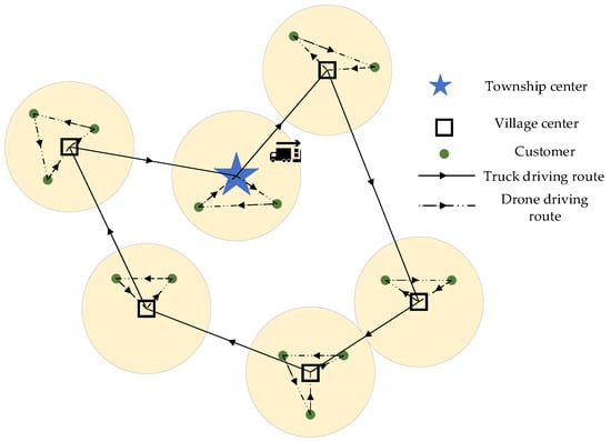
Figure 2.
Schematic diagram of the truck–drone transportation mode.
The concept of time is very important in the field of logistics. Usually, the package needs to be delivered before the specified time to meet the expectations of customers and improve service satisfaction. Considering urgent deliveries, such as medical supplies and urgent documents, different priorities will be assigned to various customers, with higher priority customers being satisfied first. The time window constraints in truck–drone logistics distribution are also taken into account, aiming to complete the delivery service before the latest expected delivery time for customers, minimizing delays in receiving goods, and enhancing the overall customer experience.
4. Mathematical Modeling
4.1. Model Assumption
In the model hypothesis, customers within the delivery distance of drones near the township distribution center are directly delivered by drones. However, for customers beyond the distance of drone transportation, the truck–drone delivery system is used for transportation. Upon the arrival of the truck at rural customer locations, a drone will be deployed for efficient distribution. Both trucks and drones are required to carry out the delivery task. The truck release drones for delivery, then stops the delivery service, waits for the drone, and then brings it back. The demand of each customer is stochastically generated within the maximum payload capacity of the drone, while taking into account the flight duration of the drone.
For achieving the lowest cost in the target, the fuel cost, labor cost, maintenance cost, and other cost factors were consolidated into two major components: the purchase cost and the fuel cost, both closely linked to the driving distance. To streamline the problem, the model design was simplified from [55,56], and the following assumptions were made:
- (1)
- The performance and load of every truck and drone are fixed.
- (2)
- A truck or a drone only serves one customer at a time.
- (3)
- The truck will not break down or be delayed during transportation, and it will not be affected by external factors such as traffic congestion.
- (4)
- The flying speed and altitude of the drone are fixed, and the driving path of the truck is processed according to the city street grid, and the driving path of the drone is a straight line.
- (5)
- The trucks and drones reach every customer, regardless of the obstacle avoidance and charging problems of the drones.
- (6)
- Trucks can only start from the distribution center, arrive at the designated customers along a delivery route, then fly the drone and finally return to the original distribution center.
4.2. Parameter Setting
The collections, parameters, and decision variables in the model are shown in Table 1.

Table 1.
Definition of collections, parameters, and decision variables.
4.3. Model Building
According to the problem description and parameter design, this is a bi−objective mixed integer programming problem, and the following model can be established.
The objective function (1) is to minimize the total cost of trucks and drones, which is the total driving cost of trucks and drones. The objective function (2) is to minimize the delivery time window lag for every customer and prioritize the requirements of high−priority customer segments to achieve optimal customer satisfaction.
Constraint (3) means that the time window period of customer is at least longer than the sum of the possible fastest arrival and service time of the drone, to avoid situations where drones consistently fail to meet user expectations.
Constraints (4) and (5) indicates that the service time of drones or trucks at customer is proportional to their demand.
Constraint (6) means that the expected earliest arrival time window of customer is at least greater than the fastest possible arrival time of the drone.
Constraint (7) uses Manhattan distance to represent the simplified representation of the truck’s delivery distance in the actual road network, and constraint (8) represents the straight−line path distance of the drone between two customers.
Constraint (9) means that for each distribution center, a truck can only leave and return once. Constraint (10) means that each drone can only leave the current delivery point once and return once, these constraints limit trucks and drones to passing by a customer only once.
Constraint (11) means that the total load of the truck must not exceed its maximum load. Constraint (12) means that the total supply of all paths of the drone does not exceed its maximum loading capacity.
Constraint (13) means that the total transportation supply of all trucks and drones is not less than the total customer demand.
Constraints (14) and (15) represent changes in the actual loading of trucks or drones during transportation.
Constraints (16) and (17) mean that the total driving mileage of each truck or each drone must not exceed its maximum driving mileage.
Constraint (18) means that for truck–drone transportation, the truck needs to wait at the current customer for the drone to complete the delivery task in the flight zone, and then go to the next customer.
Constraint (19) indicates that the demand of customer is exactly satisfied by the drone, there will never be a situation in which a single launch cannot meet the needs of customers.
5. Algorithm
The FCM model is selected for its capability in handling the uncertainties and vagueness inherent in real−world scenarios, which aligns well with the variable environmental and operational conditions of rural logistics. Its adaptability to imprecise data makes it a suitable choice for optimizing decision−making processes. At the same time, the validity of the GASA algorithm in solving the common combinatorial optimization problems in logistics routes and scheduling tasks proves its rationality. Using the simulated annealing process, GASA helps to improve time efficiency and the performance of the best cost.
5.1. FCM Algorithm
This problem is a dual−objective logistics truck–drone distribution path planning problem (CDVRPTW) with capacity constraints and time window constraints. In actual fact, the locations of distribution points in villages and towns are often determined. As pointed out in the second chapter, current rural logistics can be transported to the village level, so trucks can use these villages as temporary stops for releasing drones. The goal of the first stage is to find the delivery route of the truck.
The K−means algorithm is a clustering algorithm based on segmentation. The traditional K−means algorithm has the problem of being sensitive to the selection of the initial clustering center and having a low classification accuracy. Therefore, an improved fuzzy C−means clustering algorithm is used to divide the logistics distribution area, and the trucks are classified according to the actual positions of rural villages. The location of the distribution center determines the transportation route of the truck.
Fuzzy C−means clustering (FCM) is a soft clustering method. Its basic idea is to use membership degrees to represent the relationship between each data point, thereby determining which data point belongs to clusters. Specifically, the FCM algorithm operates on the basis of objective function. Through optimizing this function, the membership degree of each sample point to all class centers is calculated, and the class of the sample point is finally determined. The main difference between the FCM algorithm and the K−means algorithm is the way it deals with membership degrees. The K−means algorithm performs hard clustering, and the membership degree only takes 0 or 1; its goal is to minimize the sum of squared errors within the class. FCM performs fuzzy clustering with a membership value of [0, 1], aiming at minimizing the sum of squares of weighted errors within the class. Our improved FCM clustering algorithm is based on [57].
Specifically, the main steps of the improved fuzzy C−means clustering algorithm are as follows:
- (1)
- Initialization: Optimize and select sample points as the initial clustering center. Due to the sensitivity of the initial clustering center of the FCM algorithm, sample points is used to select the initial clustering center. For minimum values , let the clustering centers of the class generated by the algorithm in the th and iterations, respectively, be recorded as and . is the number of clusters, let the difference between the two be , if . Then, define the cluster center as a stable cluster center, and do not calculate the new cluster center of the class in the next iteration. Otherwise, define it as an active cluster center, and continue to calculate the new cluster center of this class in the next iteration and calculate to determine whether it is a stable cluster center. Until all clustering centers are stable clustering centers, the optimal initial clustering center is obtained.
- (2)
- Calculate the degree of membership: For each sample point, calculate its distance to each cluster center, and determine the degree to which it belongs to each cluster based on the distance. The degree of membership is as shown in Formula (20). The membership degree of the FCM algorithm refers to the membership degree of sample in class . According to the provisions of the FCM algorithm, the sum of the membership degrees of samples in each class is 1. The iterative formula for membership degree is shown in (21). The goal of the FCM algorithm is to make the objective function of Formula (22) converge to a certain value or lower than a certain threshold, or to make the difference of between the two iterations lower than a certain value or reach the specified number of iterations, at which point the operation is terminated.
- (3)
- Update clustering center: Recalculate the clustering center of each cluster based on the membership degrees of all sample points. The clustering center in FCM is different from the traditional clustering center in that it uses the membership degree as the weight to make a weighted average. The iteration formula of the cluster center is shown in (23).
- (4)
- Determine convergence: If the change in the cluster center is less than a certain threshold or reaches the maximum number of iterations then stop the iteration; otherwise, return to step (2) to continue execution.
The FCM algorithm is carried out based on the number and coordinates of samples, and the number of groups is determined. Considering the needs and priorities of the villages, the location coordinates of the cluster centers of each group are found. Then, the location of each distribution center on the truck transport route is finally determined by combining the geographical location of the center coordinates with the consideration of the existing village center factors.
5.2. Genetic Annealing Algorithm
The genetic algorithm is a random search algorithm, which simulates heredity, mutation, and other methods in evolutionary biology to search the optimal solutions. It is effective in dealing with nonlinear problems. The disadvantage of traditional genetic algorithms is that each crossover mutation search operator can only be executed once according to probability, with few choices and slow iteration speed. In the later stage of iteration, it is easy to fall into premature convergence due to excessive dependence on the parent. Genetic algorithms mainly include three steps: encoding and decoding, calculating individual fitness, and genetic operations (selection, crossover, and mutation) [58].
The simulated annealing algorithm is a probability−based optimization algorithm, which is inspired by the solid annealing principle. It takes a single individual as the object and iterates on the basis of the previous generation. The algorithm shows strong local convergence but lacks global search capability. Therefore, combining these two algorithms, a hybrid genetic simulated annealing algorithm [59,60] is designed to optimize the joint delivery route problem of truck and drones, improve the efficiency of solving, and select reasonable delivery routes until the trucks pass through all the village distribution centers and meet all customer needs. The specific operating steps of the genetic simulated annealing algorithm are as follows:
- (1)
- Set initialization parameters: population size , number of inner loops , the initial temperature , cooling coefficient λ, crossover probability , and mutation probability .
- (2)
- Generate the initial population: the truck stop numbers are sequentially encoded on chromosomes, and chromosomes of length are randomly generated ( is the number of truck stops).
- (3)
- Calculate individual fitness: The fitness function is used to measure the excellence of the chromosomes in the population. The larger the fitness value, the better the individual. The objective function is to minimize the cost, so the total operating cost of each truck and drone joint delivery solution calculated by Formula (1) is used as the fitness .
- (4)
- Genetic operators: selection operators, crossover operators, and mutation operators. The tournament method is used to select individuals with high fitness in the current population, and offspring are generated using sequential crossover with probability . To maintain the diversity of the population, individuals are mutated with probability , and the fitness of individuals in the new population is calculated as .
- (5)
- Simulated annealing operation: According to the Metropolis acceptance criterion in simulated annealing, the individuals in the new population are annealed to achieve the replacement of the old and new populations. If , the new individual will replace the old individual; otherwise, the new individual will be accepted with probability .
- (6)
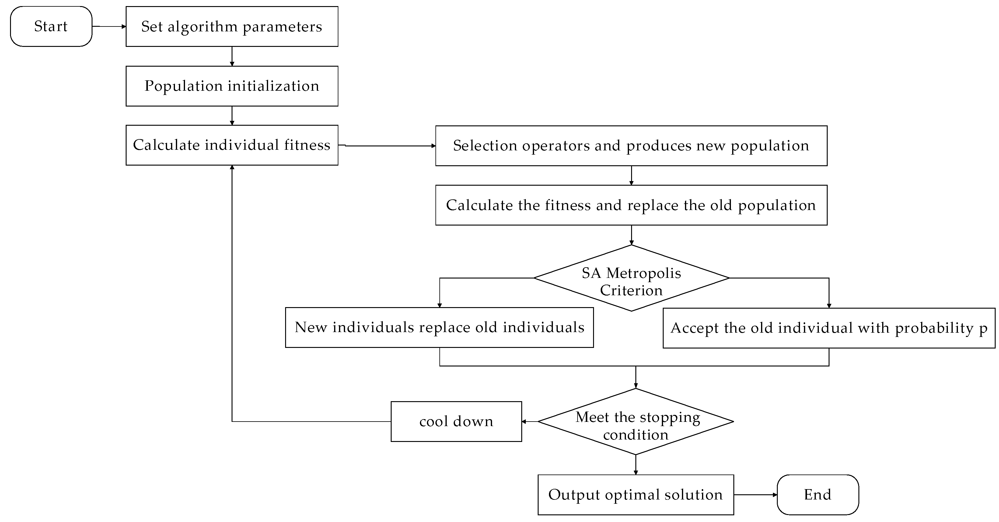
- Determine the termination condition: If the number of iterations reaches , stop the loop and output the optimal solution. Otherwise, follow to cool down and go to step (3) to continue calculation, or until the termination temperature is reached. According to the above steps, the flow chart of the genetic simulated annealing algorithm is shown in Figure 3.
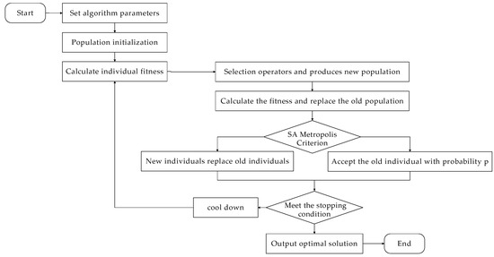 Figure 3. Genetic simulated annealing algorithm flow chart.
5.2.1. Encoding Method
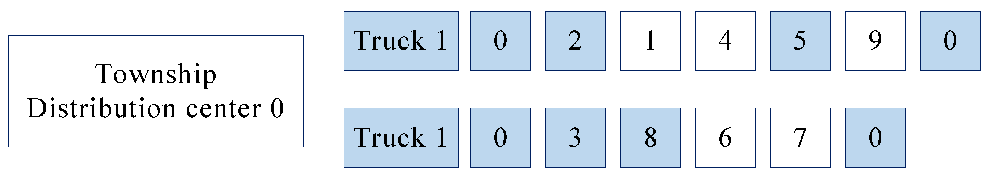
In terms of the chromosome coding method, the natural number coding method is adopted, indicates the customer and distribution center number. The node numbered represents the township distribution center. The truck starts from the node numbered and finally returns to node to complete the entire distribution task, and the number size of each point is proportional to the distance from the township distribution center.
According to the solution results of the first stage of the algorithm, the delivery route numbers of each delivery vehicle are found, in turn, to form a chromosome sequence subsequence. According to the position of the vehicle’s delivery point in the chromosome sequence, the chromosome is divided into several segments. Gene sequences within the clustering range of the truck’s delivery point are delivered by drones, and the starting point of drone delivery is the truck’s current delivery point. If the distance between the chromosome number and the township distribution center is within the delivery range of the drone, the delivery will be completed directly by the drone.
Suppose there are two delivery trucks, each of which carries out the delivery tasks while meeting the capacity and mileage restrictions. As a result of the first stage, truck 1 starts from the township distribution center and provides distribution services to rural distribution centers numbered 2 and 5. When the truck stops at the distribution center of village 2, the drone provides delivery services for customer 1 and 4 within its distribution range. Similarly, when the truck stops at the distribution center of village 5, the drone provides delivery services to customer 9 within its delivery range. Starting from the township distribution center 0, truck 2 first provides distribution services to village distribution center 3, and then provides services to village distribution center 8. This drone provides delivery services for customers 6 and 7 within its delivery range. The coding method of this hypothesis is shown in Figure 3. Trucks sequentially transport packages from left to right, and the delivery points for trucks are indicated by the same color. When the truck comes to a stop, the drone completes delivery to the respective customers. A comprehensive delivery route encompasses both the path of the truck and those of the drones. The code diagram is as shown in Figure 4.
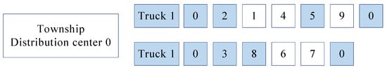
Figure 4.
Coding diagram.
5.2.2. Bequeathed Progressive Strategies
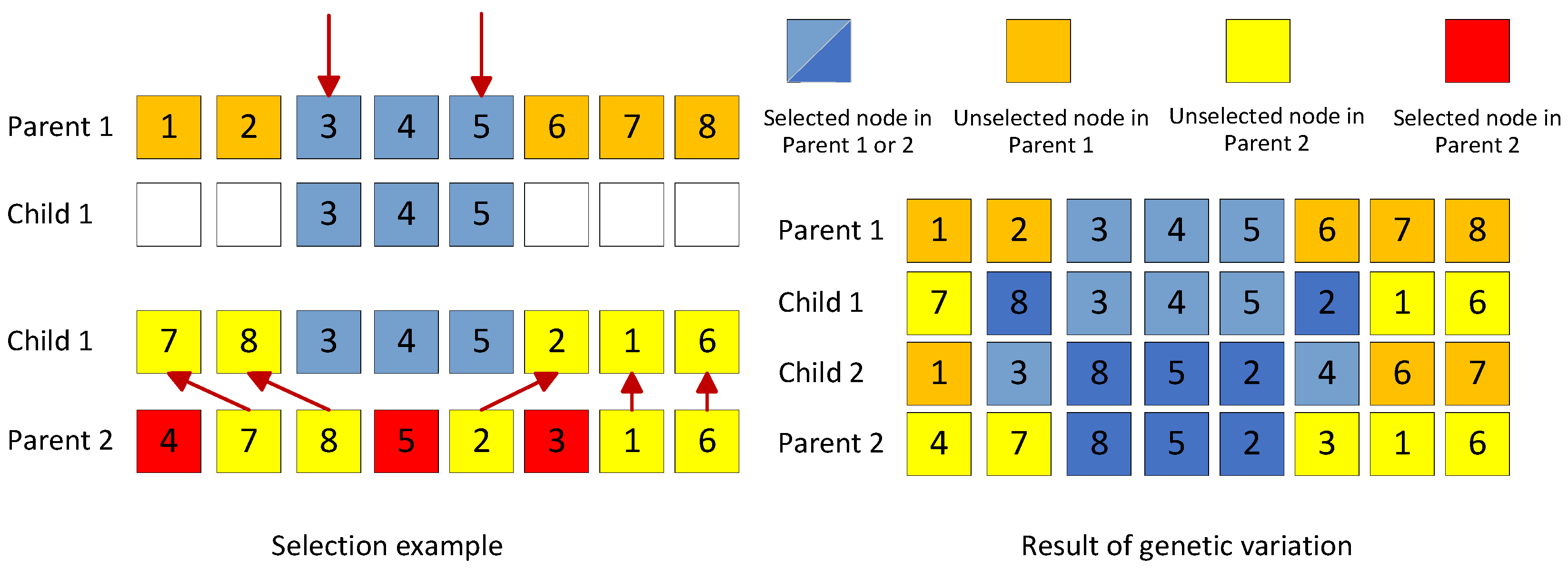
The genetic algorithm improves the search ability of the solution space through chromosome crossover operation. The selection operator is chosen through round Tournament Selection. Individuals with high fitness are selected in the current population, and then the crossover operator of sequential crossover is used. Specifically, the starting and ending positions are selected in the two parental chromosomes with probability , and the genes in this region in parental chromosome 1 are copied to the same position of offspring 1, and then the genes in parental chromosome 2 are copied to the same position. The missing genes in progeny 1 will be filled in sequence. Another descendant is also similar. The concrete operation is shown in Figure 5.
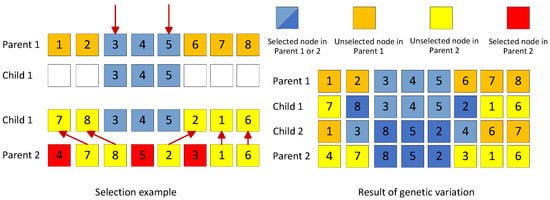
Figure 5.
Sequential crossover operator.
The mutation is helpful to improve the diversity of the solution. The object of the mutation operation is usually an individual in a population. The mutation operation is to change one or more positions in a single code string to generate new positions based on a specific mutation probability . Individuals possessing favorable genetic traits are more likely to exhibit higher rates of survival and reproductive success. Three kinds of mutation operators are used: exchange, inversion and conversion, as shown in Figure 6.
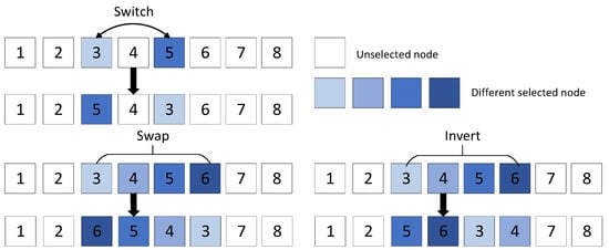
Figure 6.
Mutation operator.
Among them, exchange mutation is to randomly select two different positions on the chromosome and then exchange the consumers of these two positions. Inversion mutation is to randomly select two different positions on the chromosome, reverse the order of the coding genes between these two positions, and then insert it into the original position. Switching mutation is to first randomly select a sub−path, randomly generate two different positions on the sub−path, and randomly disrupt the order of consumers between the two positions. The two locations selected by the third mutation operations can be two locations on the same sub−path or two locations on different sub−paths, so that different paths can realize smooth exchange of information and increase the search range of the solution space.
New individuals produced by crossover and mutation are put into the corresponding population. In the selection stage, the better individuals are inherited to the next generation according to the principle of elite retention. The pseudo-code used for our algorithm is attached in Appendix A.
6. Simulation and Results Discussion
6.1. Parameter Settings
Considering the current reality of trucks and drones, trucks and drones with average performance and capacity were chosen as the data reference source for the two−stage delivery. The truck parameters used the Jiefanghu 6G light truck as a reference, and the drone parameters used the DJI FlyCart 30 as a reference. The known parameter values set are shown in Table 2.
Table 2.
Experimental factor settings.
The Huatian township, Youyang Tujia and Miao Autonomous County, Chongqing City, was selected as a pilot township. Because this area is mountainous area, traditional vehicle distribution is inefficient and costly. Therefore, the model and algorithm are simulated in this area to verify the effectiveness of the algorithm. Take a town of 1600 square kilometers as an example. The problem is simplified, resulting in a reduction in computational complexity. It is assumed that a village has an area of about 10 square kilometers, with approximately 50 villages in the township. These 50 villages are regarded as customers.
The schematic diagram of the villages of the township exported from the map is shown in Figure 7. The existing villages are used as clustering reference points, and the coordinates of the township distribution center are used as the center. The locations, needs, and time windows of all customers are known. The window is randomly generated within a given range and tries to meet the customer’s time window constraints.
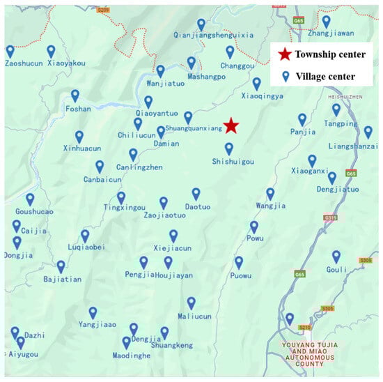
Figure 7.
Schematic diagram of the distribution of villages, towns, and villages.
The algorithm program running software is MATLAB R2023a. In the genetic simulated annealing algorithm, the population size is set to 200, the maximum number of iterations is set to 200, the crossover probability is 0.9, the mutation probability is 0.1, the initial temperature is 100, and the cooling coefficient is 0.98.
6.2. Analysis of Simulation Results
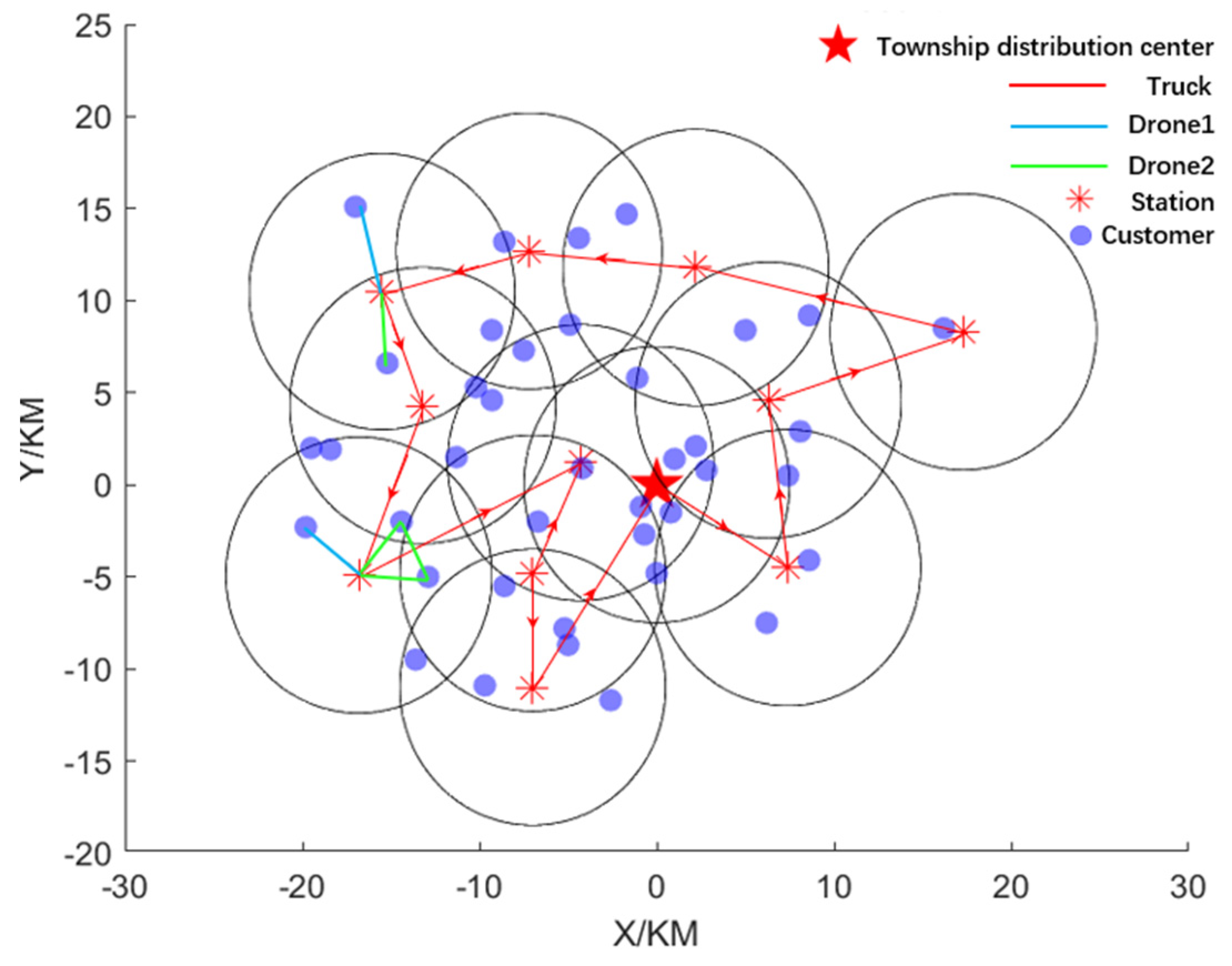
In the first stage, the improved FCM algorithm is used to cluster the 50 villages in the above cases, and the coordinates of truck parking points are obtained by combining the actual village coordinates in the cases. The coordinates of these points can actually be accessed by the trucks. In the second stage of the algorithm, after determining the driving route of the truck, the overall path planning is obtained according to the constraints conditions given above, and the results are shown in Figure 8. In order to prevent the image from being too confusing, the image only shows a clear view of the path of the truck and the delivery path of the drone leading to these two villages.
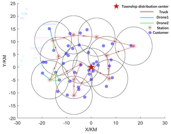
Figure 8.
Truck−drone delivery path diagram.
In Figure 8, the truck starts from the township represented by the red five−pointed star and travels along the cluster center formed by the first stage of clustering. In this process, when the truck stops at the center of a village cluster, the drone takes off to deliver goods to the villages or customers near the station and meets the constraint of the maximum distance of the drone. After the drone completes the delivery and returns to the truck, the truck will go to the cluster center in the next village for delivery. After completing all the assigned tasks, the truck will return to the township to complete the whole assignment.
The advantages of combined transportation of trucks and drones are illustrated by comparison with the transportation mode of using trucks alone. The results from Table 3 demonstrated that the two−stage delivery system utilizing trucks and drones achieves reduced travel length, delivery cost (TDC), and time window lag (TWL), compared with the only truck delivery mode. The system reduced the costs by 41.02 yuan (CNY) and saved 7.42 min. In this simulation case, two drones and a truck perform similar tasks with optimal efficiency. Drones have lower unit costs and faster flight speeds, allowing the truck–drone delivery combination to cover shorter distances compared to using trucks alone, resulting in improved cost−effectiveness and time efficiency.
Table 3.
Comparison of two−stage truck–drone and truck−only routes.
We can clearly see the optimization results of the two goals of lowest total delivery cost and minimum delayed delivery time from Figure 9. Specifically, the combined system reduces the total delivery length by 1.17%, saves 21.63% in delivery cost, and decreases delayed delivery time by 60.18% compared to the truck−only delivery. It effectively reduces the cost of logistics and transportation, reduces the lag time of parcel delivery to customers, and improves customer satisfaction.
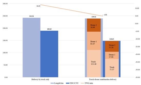
Figure 9.
Comparison results of two−stage truck−drone delivery with separate truck delivery.
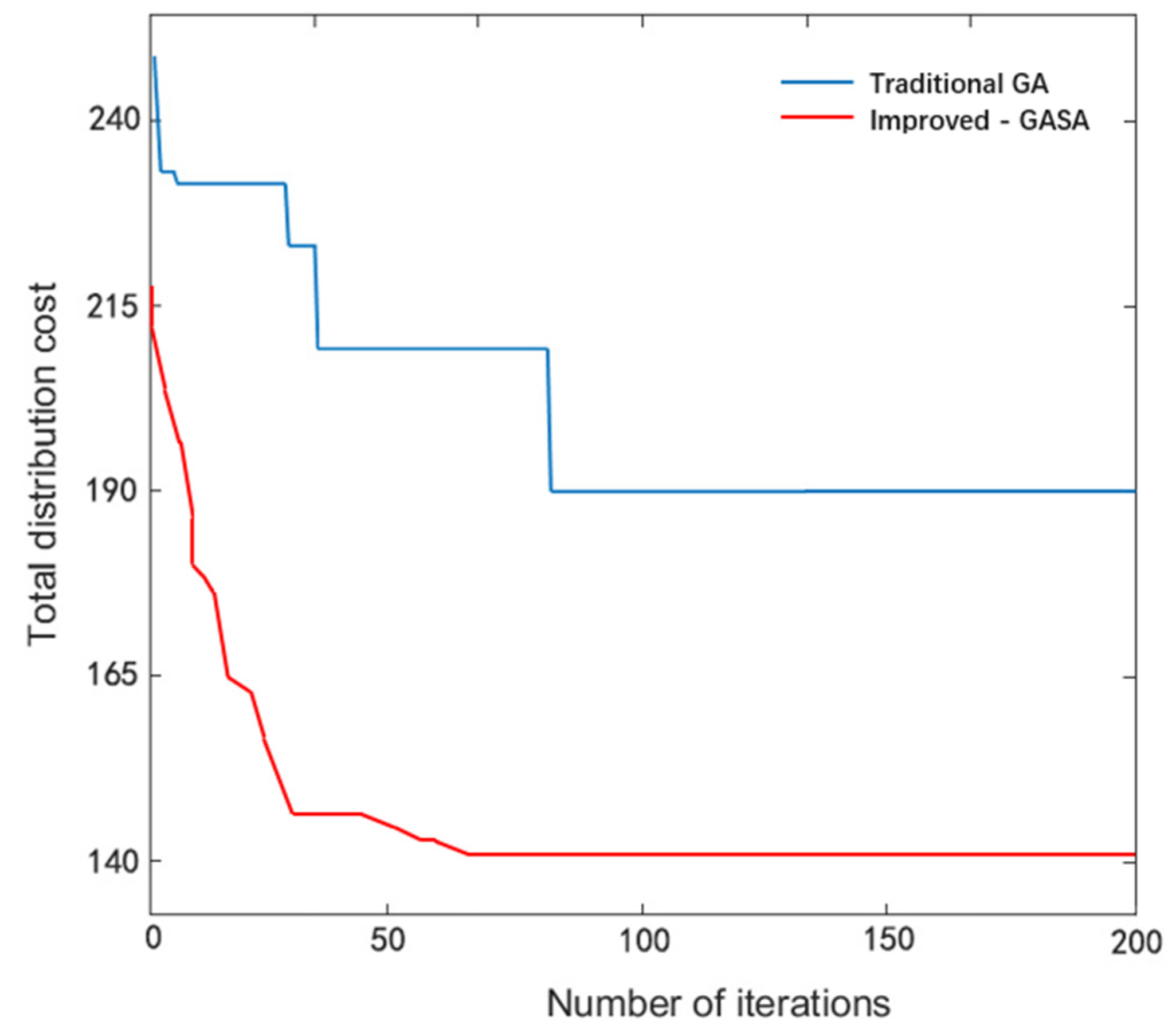
To verify the effectiveness of the proposed two−stage algorithm, the model is solved using the traditional genetic algorithm. The parameter settings remain unchanged, and the convergence performance comparison is shown in Figure 10. It can be seen from Figure 10 that the traditional genetic algorithm has more average iterations than the genetic simulated annealing algorithm, and the convergence speed is significantly slower than the improved algorithm, which means that the improved genetic simulated annealing algorithm has a higher average number of iterations in each generated solution range. It has better search accuracy and efficiency and can reach convergence faster.
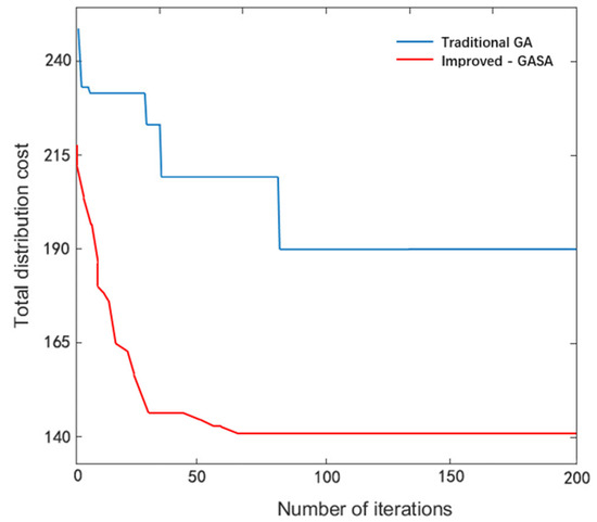
Figure 10.
Comparison of convergence performance between improved−GASA and GA.
Compared with the previous literature, a rural distribution route optimization algorithm was proposed, comprehensively considering cost and delay. This effectively reduces logistics costs and customer waiting time. Previous research did not pay attention to customer priority. The priorities of different customers are highlighted to meet personalized needs and improve delivery efficiency. Similar to previous research [61], this simulation is carried out by using real rural cases, but this research fully considered the diversity and authenticity of rural logistics. Most recent studies have used branch pricing algorithm [62] or ALNS algorithm [43] to solve the problem, but this study uses a hybrid heuristic algorithm with improved operators to make path planning more intelligent and flexible. The experimental results show that the algorithm has achieved satisfactory results in practical application and made a profound and comprehensive contribution to the research and practice of rural logistics.
7. Conclusions
The purpose of this study is to optimize the last mile logistics and solve the transportation problem in remote areas through truck–drone systems. A dual−objective logistics model of truck–drone distribution path planning considering capacity constraints and time window constraints is proposed. Due to the limited carrying and flying capacity of the UAV, trucks are used to support the transportation of the UAV and meet the logistics needs of customers. According to the characteristics of the model, the improved FCM algorithm is used to calculate the temporary stopping point of the truck in combination with the actual village coordination, and then the improved genetic operator is used to solve the truck–UAV transportation path through the genetic simulated annealing algorithm, so as to minimize the total distribution cost and delay. The feasibility of the model and algorithm are verified by an example. The results show that, compared with the traditional genetic algorithm, the improved GASA has faster convergence speed and better solving effect. The two−stage transportation mode, as compared to traditional truck transportation, yields a reduction of CNY 41.02 in total transportation cost, saves 7.42 min of time window lag, better aligns with customer time window expectations, and provides valuable insights for addressing the logistics challenges associated with last mile distribution in rural areas.
This study makes notable contributions and innovations in the realm of last mile logistics optimization in rural areas. First, the primary contribution lies in the introduction of the truck–drone delivery mode, significantly enhancing last mile logistics in rural areas. Second, the identified gap in drone applications within rural regions is effectively bridged through the proposal of a two−stage improvement algorithm, specifically designed for efficient distribution. Third, the development and application of the MILP formula represents a pivotal contribution, playing a crucial role in optimizing rural logistics. This formula takes into account the diverse priorities of customers, contributing to a more tailored and efficient distribution process. And, the study introduces advancements through the utilization of improved FCM and GASA methods in a real−life rural case. The results showcase enhanced efficiency and cost reduction, positioning these methods as superior alternatives to traditional approaches. In summary, this research not only introduces an innovative truck–drone delivery mode but also addresses existing gaps in drone applications, optimizes logistics through a sophisticated MILP formula, and demonstrates improved efficiency with advanced methods in real−world scenarios.
Nevertheless, collaborative delivery between trucks and drones faces numerous potential challenges. For instance, the logistics of dispatching and receiving drones in diverse locations are not accounted for, and technical constraints such as charging issues are not fully addressed. Variations in geographical and climatic conditions may yield different outcomes, thus necessitating careful consideration when generalizing the model. Future enhancements could leverage big data to predict customer demands and take a more comprehensive approach to addressing the technical limitations of drones in tackling last mile challenges in rural areas. Furthermore, in addition to the FCM and GASA algorithms utilized in this study, other heuristic algorithms should be considered for comparison.
Author Contributions
Conceptualization, D.D.; methodology, D.D. and H.C.; resources, L.Y.; writing—original draft, H.C.; project administration, W.S. and L.Y. All authors have read and agreed to the published version of the manuscript.
Funding
Science and Technology Commission of Shanghai Municipality (22dz1202000).
Data Availability Statement
Data are unavailable due to privacy or ethical restrictions.
Conflicts of Interest
The authors declare no conflicts of interest.
Appendix A
| Algorithm A1 Improved FCM algorithm | |
| Input: | village dataset with features (demand, distance to township); number of clusters ; convergence threshold ; |
| Output: | optimal cluster centers {} representing the final clustering solution; |
| randomly select data points from the village dataset as initial cluster centers ; | |
| compute membership matrix using the traditional FCM algorithm | |
| iterate until convergence or a maximum number of iterations | |
| compute the membership values for each village point and cluster center using the Formula (23); | |
| update the cluster centers using the Formula (25); | |
| check for convergence by calculating the change in cluster centers or membership matrix; | |
| the change is below a predefined threshold | |
| exit the iteration; | |
| set ; | |
| each cluster center | |
| set is stable = false; | |
| iterate to compute new cluster centers | |
| repeat steps 4 to 8 to update based on the membership matrix ; | |
| calculate , where is the cluster center from the previous iteration; | |
| if | |
| mark as a stable cluster center, set is stable = true; | |
| update to max(); | |
| < | |
| {}; | |
| repeat steps 2–19; | |
| Algorithm A2 Simulates genetic annealing algorithm | |
| Input: | = population size; = number of inner loops; = initial temperature; = cooling coefficient; = crossover probability; = mutation probability; num _drones = n; = num of {}; |
| % Generate the initial population | |
| chromosomes = randi ([1, ], , ); % Randomly generate chromosomes of length | |
| % Main Optimization Loop | |
| iteration = 1:M | |
| % Genetic Operations | |
| % Selection using tournament method | |
| selected _ indices = tournament _ selection (chromosomes, ); | |
| % Crossover with probability | |
| Crossover _ indices = rand (1, ) < ; | |
| offspring = sequential _ crossover (chromosomes (selected _ indices, :), crossover_indices); | |
| % Mutation with probability | |
| mutation _ indices = rand (1, N) < ; | |
| mutated _ offspring = mutate (offspring, mutation _ indices, ); | |
| % Calculate fitness for the new population | |
| new _ fitness = calculate _ fitness (mutated _ offspring); | |
| % Simulated Annealing Operation | |
| = 1: N | |
| new _ fitness () > calculate _ fitness (chromosomes (selected _indices (), :)) || rand () < exp ((calculate _ fitness (chromosomes (selected _ indices (), :))—new_fitness ()) / ) | |
| chromosomes (selected _ indices (), :) = mutated_offspring (, :); | |
| % Cooling Down | |
| = lambda × ; | |
| Output: | |
| % Find the best solution in the final population | |
| [~, best _index] = max (calculate _fitness(chromosomes)); | |
| Optimal _solution = chromosomes (best _index, :); | |
| % Separate delivery points for each drone | |
| drone _delivery _points = cell (num _drones, 1); | |
| drone = 1: num _drones then | |
| drone _delivery _points {drone} = find (optimal _solution == drone); | |
| % Output the optimal solution for each drone | |
| (‘Optimal Delivery Points for Each Drone:’); | |
| drone = 1:num_drones then | |
| (‘Drone %d: %s\n’, drone, num2str (drone _delivery _points {drone})); | |
| %Genetic Operators | |
| function selected _indices = tournament _selection (chromosomes, ) | |
| % Tournament selection function | |
| % Selects individuals with high fitness in the current population | |
| % Mutation Operators | |
| function mutated _offspring = mutate (offspring, mutation _indices, ) | |
| % Mutation function | |
| % Applies different mutation operators (switch, swap, invert) based on probabilities | |
References
- China Sees Rapid Development in Rural E-Commerce. Available online: https://english.www.gov.cn/archive/statistics/202308/15/content_WS64db757fc6d0868f4e8de941.html (accessed on 12 January 2024).
- Liu, W. Route Optimization for Last-Mile Distribution of Rural E-Commerce Logistics Based on Ant Colony Optimization. IEEE Access 2020, 8, 12179–12187. [Google Scholar] [CrossRef]
- Macioszek, E. First and Last Mile Delivery—Problems and Issues. In Advanced Solutions of Transport Systems for Growing Mobility; Sierpiński, G., Ed.; Springer International Publishing: Cham, Switzerland, 2018; pp. 147–154. [Google Scholar]
- Liang, Y.-J.; Luo, Z.-X. A Survey of Truck–Drone Routing Problem: Literature Review and Research Prospects. J. Oper. Res. Soc. China 2022, 10, 343–377. [Google Scholar] [CrossRef]
- Caraballo, L.E.; Díaz-Báñez, J.M.; Maza, I.; Ollero, A. The Block-Information-Sharing Strategy for Task Allocation: A Case Study for Structure Assembly with Aerial Robots. Eur. J. Oper. Res. 2017, 260, 725–738. [Google Scholar] [CrossRef]
- Otto, A.; Agatz, N.; Campbell, J.; Golden, B.; Pesch, E. Optimization Approaches for Civil Applications of Unmanned Aerial Vehicles (UAVs) or Aerial Drones: A Survey. Networks 2018, 72, 411–458. [Google Scholar] [CrossRef]
- Aurambout, J.-P.; Gkoumas, K.; Ciuffo, B. Last Mile Delivery by Drones: An Estimation of Viable Market Potential and Access to Citizens across European Cities. Eur. Transp. Res. Rev. 2019, 11, 30. [Google Scholar] [CrossRef]
- Tokosh, J.; Chen, X. Delivery by Drone: Estimating Market Potential and Access to Consumers from Existing Amazon Infrastruture. Pap. Appl. Geogr. 2022, 8, 414–433. [Google Scholar] [CrossRef]
- Rejeb, A.; Rejeb, K.; Simske, S.J.; Treiblmaier, H. Drones for Supply Chain Management and Logistics: A Review and Research Agenda. Int. J. Logist. Res. Appl. 2023, 26, 708–731. [Google Scholar] [CrossRef]
- Murray, C.C.; Chu, A.G. The Flying Sidekick Traveling Salesman Problem: Optimization of Drone-Assisted Parcel Delivery. Transp. Res. Part C Emerg. Technol. 2015, 54, 86–109. [Google Scholar] [CrossRef]
- Drexl, M. Synchronization in Vehicle Routing—A Survey of VRPs with Multiple Synchronization Constraints. Transp. Sci. 2012, 46, 297–316. [Google Scholar] [CrossRef]
- El-Adle, A.M.; Ghoniem, A.; Haouari, M. The Cost of Carrier Consistency: Last-Mile Delivery by Vehicle and Drone for Subscription-Based Orders. J. Oper. Res. Soc. 2023, 1–20. [Google Scholar] [CrossRef]
- Zou, B.; Wu, S.; Gong, Y.; Yuan, Z.; Shi, Y. Delivery Network Design of a Locker-Drone Delivery System. Int. J. Prod. Res. 2023, 1–25. [Google Scholar] [CrossRef]
- Pan, J.-S.; Song, P.-C.; Chu, S.-C.; Peng, Y.-J. Improved Compact Cuckoo Search Algorithm Applied to Location of Drone Logistics Hub. Mathematics 2020, 8, 333. [Google Scholar] [CrossRef]
- Yang, F.; Dai, Y.; Ma, Z.-J. A Cooperative Rich Vehicle Routing Problem in the Last-Mile Logistics Industry in Rural Areas. Transp. Res. Part E Logist. Transp. Rev. 2020, 141, 102024. [Google Scholar] [CrossRef]
- Nikolić, I.; Milutinović, J.; Božanić, D.; Dobrodolac, M. Using an Interval Type-2 Fuzzy AROMAN Decision-Making Method to Improve the Sustainability of the Postal Network in Rural Areas. Mathematics 2023, 11, 3105. [Google Scholar] [CrossRef]
- Niemeijer, R.; Buijs, P. A Greener Last Mile: Analyzing the Carbon Emission Impact of Pickup Points in Last-Mile Parcel Delivery. Renew. Sustain. Energy Rev. 2023, 186, 113630. [Google Scholar] [CrossRef]
- Nadimuthu, L.P.R.; Victor, K. Environmental Friendly Micro Cold Storage for Last-Mile Covid-19 Vaccine Logistics. Environ. Sci. Pollut. Res. 2022, 29, 23767–23778. [Google Scholar] [CrossRef] [PubMed]
- Yang, T.; Chu, Z.; Wang, B. Feasibility on the Integration of Passenger and Freight Transportation in Rural Areas: A Service Mode and an Optimization Model. Socio-Econ. Plan. Sci. 2023, 88, 101665. [Google Scholar] [CrossRef]
- Jiang, X.; Wang, H.; Guo, X.; Gong, X. Using the FAHP, ISM, and MICMAC Approaches to Study the Sustainability Influencing Factors of the Last Mile Delivery of Rural E-Commerce Logistics. Sustainability 2019, 11, 3937. [Google Scholar] [CrossRef]
- Kou, X.; Zhang, Y.; Long, D.; Liu, X.; Qie, L. An Investigation of Multimodal Transport for Last Mile Delivery in Rural Areas. Sustainability 2022, 14, 1291. [Google Scholar] [CrossRef]
- Dorling, K.; Heinrichs, J.; Messier, G.G.; Magierowski, S. Vehicle Routing Problems for Drone Delivery. IEEE Trans. Syst. Man Cybern. Syst. 2017, 47, 70–85. [Google Scholar] [CrossRef]
- Rabta, B.; Wankmüller, C.; Reiner, G. A Drone Fleet Model for Last-Mile Distribution in Disaster Relief Operations. Int. J. Disaster Risk Reduct. 2018, 28, 107–112. [Google Scholar] [CrossRef]
- Shao, J.; Cheng, J.; Xia, B.; Yang, K.; Wei, H. A Novel Service System for Long-Distance Drone Delivery Using the “Ant Colony+A*” Algorithm. IEEE Syst. J. 2021, 15, 3348–3359. [Google Scholar] [CrossRef]
- Yuan, X.; Zhu, J.; Li, Y.; Huang, H.; Wu, M. An Enhanced Genetic Algorithm for Unmanned Aerial Vehicle Logistics Scheduling. IET Commun. 2021, 15, 1402–1411. [Google Scholar] [CrossRef]
- Wang, Y.; Wang, L.; Peng, Z.; Chen, G.; Cai, Z.; Xing, L. A Multi Ant System Based Hybrid Heuristic Algorithm for Vehicle Routing Problem with Service Time Customization. Swarm Evol. Comput. 2019, 50, 100563. [Google Scholar] [CrossRef]
- Spliet, R.; Dabia, S.; Van Woensel, T. The Time Window Assignment Vehicle Routing Problem with Time-Dependent Travel Times. Transp. Sci. 2018, 52, 261–276. [Google Scholar] [CrossRef]
- Hossain, N.U.I.; Nur, F.; Hosseini, S.; Jaradat, R.; Marufuzzaman, M.; Puryear, S.M. A Bayesian Network Based Approach for Modeling and Assessing Resilience: A Case Study of a Full Service Deep Water Port. Reliab. Eng. Syst. Saf. 2019, 189, 378–396. [Google Scholar] [CrossRef]
- Ha, Q.M.; Deville, Y.; Pham, Q.D.; Hà, M.H. On the Min-Cost Traveling Salesman Problem with Drone. Transp. Res. Part C Emerg. Technol. 2018, 86, 597–621. [Google Scholar] [CrossRef]
- Kirschstein, T. Comparison of Energy Demands of Drone-Based and Ground-Based Parcel Delivery Services. Transp. Res. Part D Transp. Environ. 2020, 78, 102209. [Google Scholar] [CrossRef]
- Raghunatha, A.; Lindkvist, E.; Thollander, P.; Hansson, E.; Jonsson, G. Critical Assessment of Emissions, Costs, and Time for Last-Mile Goods Delivery by Drones versus Trucks. Sci. Rep. 2023, 13, 11814. [Google Scholar] [CrossRef]
- Elsayed, M.; Mohamed, M. The Impact of Airspace Regulations on Unmanned Aerial Vehicles in Last-Mile Operation. Transp. Res. Part D Transp. Environ. 2020, 87, 102480. [Google Scholar] [CrossRef]
- Kim, S.; Moon, I. Traveling Salesman Problem With a Drone Station. IEEE Trans. Syst. Man Cybern. Syst. 2019, 49, 42–52. [Google Scholar] [CrossRef]
- Enthoven, D.L.J.U.; Jargalsaikhan, B.; Roodbergen, K.J.; uit het Broek, M.A.J.; Schrotenboer, A.H. The Two-Echelon Vehicle Routing Problem with Covering Options: City Logistics with Cargo Bikes and Parcel Lockers. Comput. Oper. Res. 2020, 118, 104919. [Google Scholar] [CrossRef]
- Park, J.; Kim, S.; Suh, K. A Comparative Analysis of the Environmental Benefits of Drone-Based Delivery Services in Urban and Rural Areas. Sustainability 2018, 10, 888. [Google Scholar] [CrossRef]
- Kim, S.J.; Lim, G.J.; Cho, J.; Côté, M.J. Drone-Aided Healthcare Services for Patients with Chronic Diseases in Rural Areas. J. Intell. Robot. Syst. 2017, 88, 163–180. [Google Scholar] [CrossRef]
- Moshref-Javadi, M.; Hemmati, A.; Winkenbach, M. A Truck and Drones Model for Last-Mile Delivery: A Mathematical Model and Heuristic Approach. Appl. Math. Model. 2020, 80, 290–318. [Google Scholar] [CrossRef]
- Kitjacharoenchai, P.; Ventresca, M.; Moshref-Javadi, M.; Lee, S.; Tanchoco, J.M.A.; Brunese, P.A. Multiple Traveling Salesman Problem with Drones: Mathematical Model and Heuristic Approach. Comput. Ind. Eng. 2019, 129, 14–30. [Google Scholar] [CrossRef]
- Wang, D.; Hu, P.; Du, J.; Zhou, P.; Deng, T.; Hu, M. Routing and Scheduling for Hybrid Truck-Drone Collaborative Parcel Delivery With Independent and Truck-Carried Drones. IEEE Internet Things J. 2019, 6, 10483–10495. [Google Scholar] [CrossRef]
- Silva, D.F.; Smith, A.E. Sustainable Last Mile Parcel Delivery and Return Service Using Drones. Eng. Appl. Artif. Intell. 2023, 124, 106631. [Google Scholar] [CrossRef]
- Zhou, H.; Qin, H.; Zhang, Z.; Li, J. Two-Echelon Vehicle Routing Problem with Time Windows and Simultaneous Pickup and Delivery. Soft Comput. 2022, 26, 3345–3360. [Google Scholar] [CrossRef]
- Salama, M.; Srinivas, S. Joint Optimization of Customer Location Clustering and Drone-Based Routing for Last-Mile Deliveries. Transp. Res. Part C Emerg. Technol. 2020, 114, 620–642. [Google Scholar] [CrossRef]
- Rave, A.; Fontaine, P.; Kuhn, H. Drone Location and Vehicle Fleet Planning with Trucks and Aerial Drones. Eur. J. Oper. Res. 2023, 308, 113–130. [Google Scholar] [CrossRef]
- Karakatič, S.; Podgorelec, V. A Survey of Genetic Algorithms for Solving Multi Depot Vehicle Routing Problem. Appl. Soft Comput. 2015, 27, 519–532. [Google Scholar] [CrossRef]
- Prajapati, D.; Chan, F.T.S.; Daultani, Y.; Pratap, S. Sustainable Vehicle Routing of Agro-Food Grains in the e-Commerce Industry. Int. J. Prod. Res. 2022, 60, 7319–7344. [Google Scholar] [CrossRef]
- Ha, Q.M.; Deville, Y.; Pham, Q.D.; Hà, M.H. A Hybrid Genetic Algorithm for the Traveling Salesman Problem with Drone. J. Heuristics 2020, 26, 219–247. [Google Scholar] [CrossRef]
- Sacramento, D.; Pisinger, D.; Ropke, S. An Adaptive Large Neighborhood Search Metaheuristic for the Vehicle Routing Problem with Drones. Transp. Res. Part C Emerg. Technol. 2019, 102, 289–315. [Google Scholar] [CrossRef]
- Euchi, J.; Sadok, A. Hybrid Genetic-Sweep Algorithm to Solve the Vehicle Routing Problem with Drones. Phys. Commun. 2021, 44, 101236. [Google Scholar] [CrossRef]
- Wang, Y.; Yang, X.; Chen, Z. An Efficient Hybrid Graph Network Model for Traveling Salesman Problem with Drone. Neural Process Lett. 2023, 55, 10353–10370. [Google Scholar] [CrossRef]
- Wu, X.; Yin, Y.; Xu, L.; Wu, X.; Meng, F.; Zhen, R. MULTI-UAV Task Allocation Based on Improved Genetic Algorithm. IEEE Access 2021, 9, 100369–100379. [Google Scholar] [CrossRef]
- Zhou, Z.; Luo, D.; Shao, J.; Xu, Y.; You, Y. Immune Genetic Algorithm Based Multi-UAV Cooperative Target Search with Event-Triggered Mechanism. Phys. Commun. 2020, 41, 101103. [Google Scholar] [CrossRef]
- Tan, Y.; Li, S.; Liu, H.; Chen, P.; Zhou, Z. Automatic Inspection Data Collection of Building Surface Based on BIM and UAV. Autom. Constr. 2021, 131, 103881. [Google Scholar] [CrossRef]
- Ferrandez, S.M.; Harbison, T.; Weber, T.; Sturges, R.; Rich, R. Optimization of a Truck-Drone in Tandem Delivery Network Using k-Means and Genetic Algorithm. J. Ind. Eng. Manag. 2016, 9, 374–388. [Google Scholar] [CrossRef]
- Chang, Y.S.; Lee, H.J. Optimal Delivery Routing with Wider Drone-Delivery Areas along a Shorter Truck-Route. Expert Syst. Appl. 2018, 104, 307–317. [Google Scholar] [CrossRef]
- Cavani, S.; Iori, M.; Roberti, R. Exact Methods for the Traveling Salesman Problem with Multiple Drones. Transp. Res. Part C Emerg. Technol. 2021, 130, 103280. [Google Scholar] [CrossRef]
- Song, B.D.; Park, K.; Kim, J. Persistent UAV Delivery Logistics: MILP Formulation and Efficient Heuristic. Comput. Ind. Eng. 2018, 120, 418–428. [Google Scholar] [CrossRef]
- Saxena, A.; Prasad, M.; Gupta, A.; Bharill, N.; Patel, O.P.; Tiwari, A.; Er, M.J.; Ding, W.; Lin, C.-T. A Review of Clustering Techniques and Developments. Neurocomputing 2017, 267, 664–681. [Google Scholar] [CrossRef]
- Dokeroglu, T.; Sevinc, E.; Kucukyilmaz, T.; Cosar, A. A Survey on New Generation Metaheuristic Algorithms. Comput. Ind. Eng. 2019, 137, 106040. [Google Scholar] [CrossRef]
- Chen, P.-H.; Shahandashti, S.M. Hybrid of Genetic Algorithm and Simulated Annealing for Multiple Project Scheduling with Multiple Resource Constraints. Autom. Constr. 2009, 18, 434–443. [Google Scholar] [CrossRef]
- Yu, V.F.; Aloina, G.; Susanto, H.; Effendi, M.K.; Lin, S.-W. Regional Location Routing Problem for Waste Collection Using Hybrid Genetic Algorithm-Simulated Annealing. Mathematics 2022, 10, 2131. [Google Scholar] [CrossRef]
- Enayati, S.; Li, H.; Campbell, J.F.; Pan, D. Multimodal Vaccine Distribution Network Design with Drones. Transp. Sci. 2023, 57, 1069–1095. [Google Scholar] [CrossRef]
- Levin, M.W.; Rey, D. Branch-and-Price for Drone Delivery Service Planning in Urban Airspace. Transp. Sci. 2023, 57, 843–865. [Google Scholar] [CrossRef]


Disclaimer/Publisher’s Note: The statements, opinions and data contained in all publications are solely those of the individual author(s) and contributor(s) and not of MDPI and/or the editor(s). MDPI and/or the editor(s) disclaim responsibility for any injury to people or property resulting from any ideas, methods, instructions or products referred to in the content. |
© 2024 by the authors. Licensee MDPI, Basel, Switzerland. This article is an open access article distributed under the terms and conditions of the Creative Commons Attribution (CC BY) license (https://creativecommons.org/licenses/by/4.0/).