Parameterization and Performance Analysis of a Scalable, near Real-Time Packet Capturing Platform

Abstract

The rapid evolution of technology has fostered an exponential rise in the number of individuals and devices interconnected via the Internet. This interconnectedness has prompted companies to expand their computing and communication infrastructures significantly to accommodate the escalating demands. However, this proliferation of connectivity has also opened new avenues for cyber threats, emphasizing the critical need for Intrusion Detection Systems (IDSs) to adapt and operate efficiently in this evolving landscape. In response, companies are increasingly seeking IDSs characterized by horizontal, modular, and elastic attributes, capable of dynamically scaling with the fluctuating volume of network data flows deemed essential for effective monitoring and threat detection. Yet, the task extends beyond mere data capture and storage; robust IDSs must integrate sophisticated components for data analysis and anomaly detection, ideally functioning in real-time or near real-time. While Machine Learning (ML) techniques present promising avenues for detecting and mitigating malicious activities, their efficacy hinges on the availability of high-quality training datasets, which in turn poses a significant challenge. This paper proposes a comprehensive solution in the form of an architecture and reference implementation for (near) real-time capture, storage, and analysis of network data within a 1 Gbps network environment. Performance benchmarks provided offer valuable insights for prototype optimization, demonstrating the capability of the proposed IDS architecture to meet objectives even under realistic operational scenarios.

1. Introduction

Cyberattacks have represented a security issue for many years and are continuously becoming more sophisticated, increasing in difficulty for prevention and detection. Companies that rely on Internet-connected IT infrastructures (nowadays, the vast majority, if not all) should have in place counter-measure systems, as those attacks may have devastating consequences in case of a breach (e.g., ex-filtration, tampering, destruction or encryption of data) [1].

To prevent and detect these incidents, IDSs capable of analyzing network traffic in (near) real-time are needed. As cyberattacks are growing in number and complexity, as well as network links speeds, traditional IDSs may not be effective anymore, requiring more scalable and robust components, as well as the coupling with novel data analysis techniques, namely from the ML domain [2].

In previous work [3], an architecture for such a kind of IDS was already introduced. This also included an in-depth statement of the problem under consideration and the selection of the technologies for a reference implementation of the proposed architecture.

This paper goes further, by focusing on the experimental evaluation of an architecture prototype that embodies the reference implementation. The testbed deployed captures raw network data that flows through switching devices on an Ethernet network, at the line rate of 1 Gbps, and sends the data to others modules, which are responsible for data storage and analysis in (near) real-time. Several experiments were conducted, aiming to gain insight on the best values (performance-wise) of critical parameters of the prototype components and assess the capability of performing (near) real-time operation.

Indeed, the design of such a solution requires, right from the start, careful consideration of numerous factors that may affect its performance. Hence, utmost care must be given to the selection of technologies and its precise parameterization. Therefore, this manuscript describes a systematic methodology designed to evaluate a spectrum of parameters with the goal of identifying the most performant configuration for our IDS implementation.

The remainder of this paper is organized as follows: Section 2 sums up the proposed architecture and the technologies chosen for its prototyping; Section 3 describes the experimental testbed and the methodology pursued; Section 4 presents the experimental results and associated discussion; finally, Section 5 concludes and lays out future work directions.

2. Methods and Materials

As already stated, the architecture and technological choices for the IDS evaluated in this paper were previously defined in [3]. A summary of its main aspects follows.

2.1. Architecture

The system architecture was designed to be modular and horizontally scalable. This implies the possibility of modifying/replacing a system component with none (or very minor) changes to the other components. It also means that it should be possible to add, in a transparent way, new service units, in order to accommodate extra levels of performance, storage and availability, whenever required.

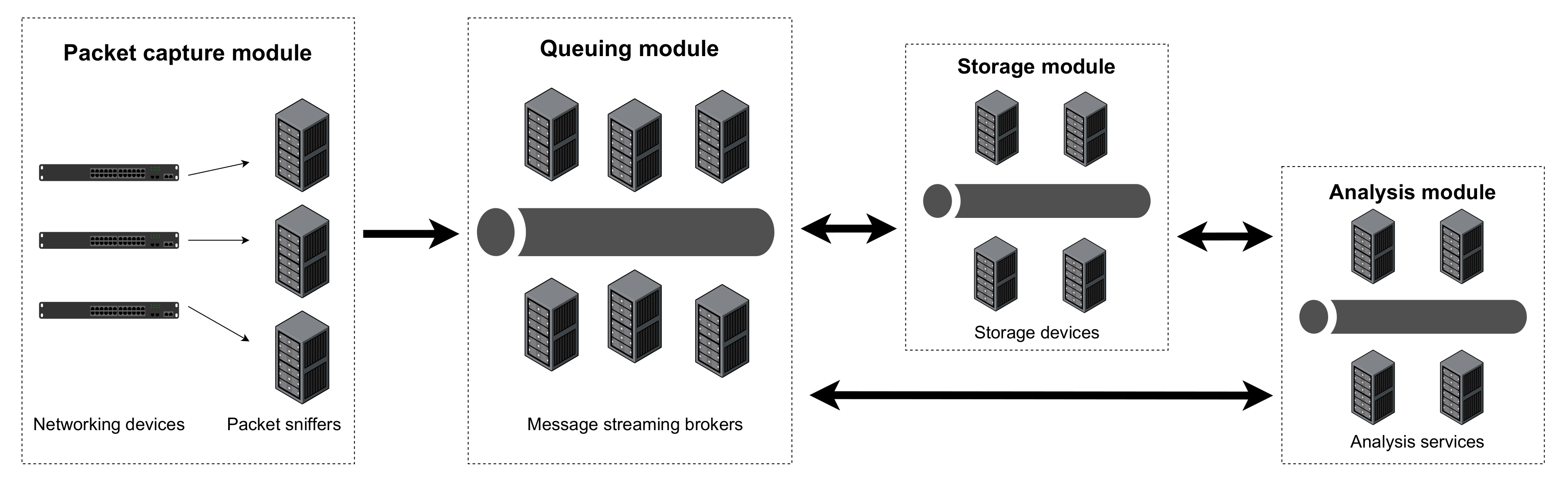
Figure 1 presents an overview of the proposed architecture, which includes four different modules or components. A description of their role and interactions follows.

It all starts at the packet capture module, which is composed of network sniffers, also known as probes. Each probe is connected to a switch with port-mirroring configured, in order to replicate incoming traffic to the port where the probe is attached to. Each probe captures every network packet that reaches its Network Card Interface (NIC). These packets are then published to the messaging system operated by the queuing module.

During a network capture, the data published to the queuing module may be consumed by the storage module and/or by the analysis module. Using a queuing mechanism naturally supports the simultaneous operation of multiple producers (probes) and multiple consumers, increasing the IDS throughput. In particular, more network traffic may be captured, and the acquired data may be split to allow parallel storage and/or processing.

The queuing module can hold data for a limited amount of time, before exhausting its limited internal storage capacity. When local storage runs out, newly arrived messages may be lost, or older messages may be discarded to make room for the new messages, depending on the behavior configured. So that all network data captured is preserved, the storage module consumes all data gathered by the queuing module and saves it in a persistent distributed storage repository. This way, if further analyses are required on specific data segments, the storage module is capable of republishing the required data to the queuing module, so that it may be consumed by the analysis module.

The analysis module may be able to consume data in (near) real-time from the queuing module, as it is published there by the packet capture module. It may also be able to consume data directly from the storage module, if such is found to be more convenient and/or efficient. The analysis at stake may be conducted based on different technologies and approaches, such as machine learning algorithms, clustering techniques, visualization dashboards, etc. Different options may coexist and each option may be supported by several service instances in order to split the load involved and offer increased performance.

2.2. Tools and Technologies

When implementing a system to perform an efficient analysis of possibly huge chunks of data, selecting the appropriate technologies and tools is halfway towards a solid final system [4].

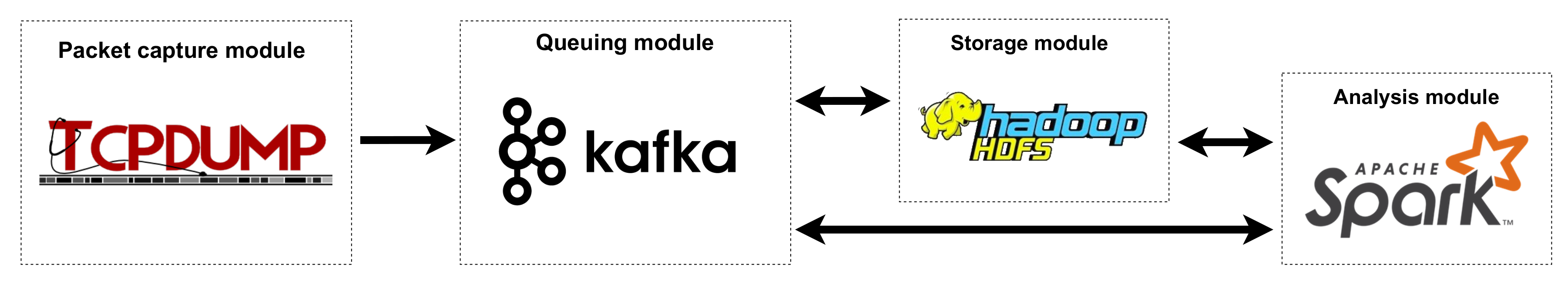
Based on the architecture presented in Figure 1, a literature review followed, allowing to choose the best tools and technologies to support each architecture module. As represented in Figure 2, the choices landed on tcpdump for the packet capture module, Apache Kafka for the queuing module, Apache HDFS for the storage module, and Apache Spark for the analysis module. The literature review that led to these choices is presented next.

2.2.1. Network Capture

The selection of a network packet capture tool is always a challenging task. A capturing tool should have zero (or very low) packet loss rate while capturing packets in a multi-Gbps rate network. It is also desirable that such tools are open-source and, if possible, free of charge. Several examples, that cope differently with these requisites, are provided next.

Scapy is a Python framework for packet capture [5]. Although it is very easy to use, Scapy-based applications have limited performance: they cannot reach multi-Gbps capture rates and suffer from very high CPU usage, thus leaving almost no processing resources available to perform other important operations.

nProbe is a capturing tool that applies PF_Ring to reach up to 100 Gbps rates while capturing network packets [6], but it is not free and thus was not considered for this work.

D. Álvarez et al. [7] performed a CPU usage comparison between TCPDump [8], Wireshark [8] and Tshark [9] when sniffing the network. While TCPDump kept an average of 1% of CPU usage, Wireshark and Tshark used 100% and 55%, respectively. As such, TCPDump was selected as the network packet capture tool for our IDS. Since TCPDump works on top of the libpcap framework, it utilizes a zero-copy mechanism, reducing the data copies and system calls, and consequently improving the overall performance [10].

2.2.2. Data Streaming

Event streaming is the practice of capturing data in real-time from one or multiple sources, and storing it for later retrieval. It works based on the publish-subscribe model, where producers publish to a distributed queue and consumers subscribe to obtain the data when available. The data streaming component (queuing module) of our architecture relies on Apache Kafka [11], a community project maintained by the Apache software foundation.

Kafka runs as a cluster of one or more service instances that can be placed on multiple hosts. Some instances, named brokers, form the storage layer, while others continuously import and export data as event streams to integrate Kafka with other existing systems. A Kafka cluster offers fault tolerance: if any instance fails, other will take over its work, ensuring continuous operation without data loss [12]. Other Kafka features include:

• Events are organised and stored in topics, and can be consumed as often as needed;
• A topic can have zero or multiple producers and consumers;
• Topics are partitioned, allowing a topic to be dispersed by several “buckets” located on different (or the same) Kafka brokers;
• A topic can be replicated into other brokers; this way, multiple brokers have a copy of the data, allowing the automatic failover to these replicas when an instance fails;
• Performance is constant regardless of the data size;
• Kakfa uses the pull model, by which consumers request and fetch the data from the queue, instead of the data being pushed to the consumers.

D. Surekha et al. [13] and S. Mousavi et al. [6] use Kafka on their systems due to being a scalable and reliable messaging system with excellent throughput and fault tolerance, which are Qualities-of-Service (QoSs) specially relevant in the context of our IDS.

Apache Flume [14] and Amazon Kinesis [15] were pondered as possible alternatives to Kafka, but they have some characteristics that make them unsuitable to our IDS. Apache Flume offers features similar to Kafka’s but it uses the push model, whereby instead of being the consumer that fetches the data, it is the service that forwards the data to the consumer; moreover, the push of messages may happen regardless if the consumers are ready or not to receive them. Amazon Kinesis can handle hundreds of terabytes per hour of real-time data flow, but it is a cloud-based solution, thus to be deployed in an environment not currently targeted by our IDS (which focus mainly on private corporate networks).

2.2.3. Persistent Storage

The platform adopted for the storage module was the Hadoop Distributed File System (HDFS) [16]. This platform is one of the 60 components of the Apache Hadoop ecosystem, having the ability to store large files in a distributed way (split in chunks across multiple nodes), while offering reliability and extreme fault-tolerance. Being based on the Google File System [17], HDFS is tailored to a write-once-read-many [18] usage pattern.

HDFS builds on two main entities: (i) one or more NameNodes and (ii) several DataNodes. A NameNode stores the metadata of the files and the location of their chunks. Chunks become replicated across the DataNodes, reducing the risk of losing data. The DataNodes are responsible for the storage and retrieval of data blocks as needed [19].

There are many HDFS use-cases for real-time scenarios (though none that we could find matching to our specific purpose). K. Madhu et al. [20], S. Mishra et al. [21], K. Aziz et al. [22] and R. Kamal et al. [23] all perform real-time data analysis on tweets from Twitter that are stored in HDFS. S. Kumar et al. [14] use HDFS to store real-time massive amounts of data produced by autonomous vehicles sensors. J. Tsai et al. [24] undertake the analysis of real-time road traffic to estimate future road traffic with the data stored in HDFS.

Several alternatives to HDFS were also considered, including Ceph [25] and GlusterFS [26]. Ceph is a reliable, scalable, fault-tolerant and distributed storage system, allowing not only to store files but also objects and blocks. GlusterFS is a scalable file-system capable of storing petabytes of data in a distributed way. C. Yang et al. [27] compared HDFS, GlusterFS and Ceph performance while writing and reading files. According to their results, the performance of HDFS is superior to the other two platforms.

2.2.4. Data Process

Among other alternatives, Apache Spark [28] was the one selected for the data processing/analysis component. Apache Spark provides a high-level abstraction representing a continuous flow of data [29]. It receives the data from diverse sources, such as Apache Kafka and Amazon Kinesis, and then processes it as micro-batches [4]. Apache Spark is implemented in Scala and runs on the Java Virtual Machine (JVM). It provides two options to run algorithms: (i) as an interpreter of Scala, Python or R code, that allows users to run queries on large databases; (ii) to write applications on Scala and upload them to the master node for execution [30]. Some usage scenarios of Apache Spark are provided next.

S. Mishra et al. [31] proposed a framework to predict congestion on multivariate IoT data streams in a smart city scenario, using Apache Spark to receive and process data from Apache Kafka. A. Saraswathi et al. [32] also used Kafka and Spark to predict road traffic in real-time. Y. Drohobytskiy et al. [33] developed a real-time multi-party data exchange using Apache Spark to obtain data from Apache Kafka, process it and store it in HDFS.

Apache Storm is a free, open-source real-time computation system capable of real-time data processing [34], just like Apache Spark streaming. J. Karimov et al. [35] and Z. Karakaya et al. [36] both performed an experiment comparing Apache Storm, Apache Flink and Apache Spark. Based on the results, they concluded that Apache Spark outperforms Apache Storm, being better at processing incoming streaming data in real-time. Between Apache Spark Streaming and Apache Flink, the choice is more difficult: they exhibit similar results in benchmarks, but they both have their own pros and cons.

According to the experiments of M. Tun et al. [37], the integration of Apache Kafka and Apache Spark streaming can improve the processing time and the fault-tolerance when dealing with huge amounts of data. Thus, Apache Spark streaming was selected for this work, once it integrates well with Apache Kafka, supporting real-time operations.

Also, Apache Spark uses in-memory operations to perform stream processing, and it recovers from node failure without any loss—something that Apache Flink and Apache Storm are not able to offer [37]. Moreover, data can be acquired from multiple different sources, like Apache Kafka, Apache Flume, Amazon Kinesis, etc.

Another alternative considered was Apache Hadoop MapReduce, based on Googles’ MapReduce [38]. This is a framework for writing programs that process multi-terabyte datasets in parallel on multi nodes, offering reliability and fault-tolerance [39]. However, Apache Spark is up to 100 times faster than MapReduce since it uses in-memory processing for large parallel processing [37] while MapReduce performs disk-based operations. MapReduce’s approach to tracking tasks is based on heartbeats causing an unnecessary delay while Apache Spark is event-driven [40].

Hence, compared with MapReduce, Apache Spark suits better our scenario, as it focuses on the processing speed, while MapReduce focuses on dealing with massive amounts of data [29]. Moreover, Apache Spark contains a vast amount of libraries to support data analysis. Also, other applications in addition to Spark jobs (Python scripts) may be deployed and implemented in the analysis workflow.

3. Experimental Testbed and Methodology

This section describes the experimental testbed assembled, and the evaluation methodology followed, to assess a prototype of the proposed IDS architecture.

3.1. Testbed

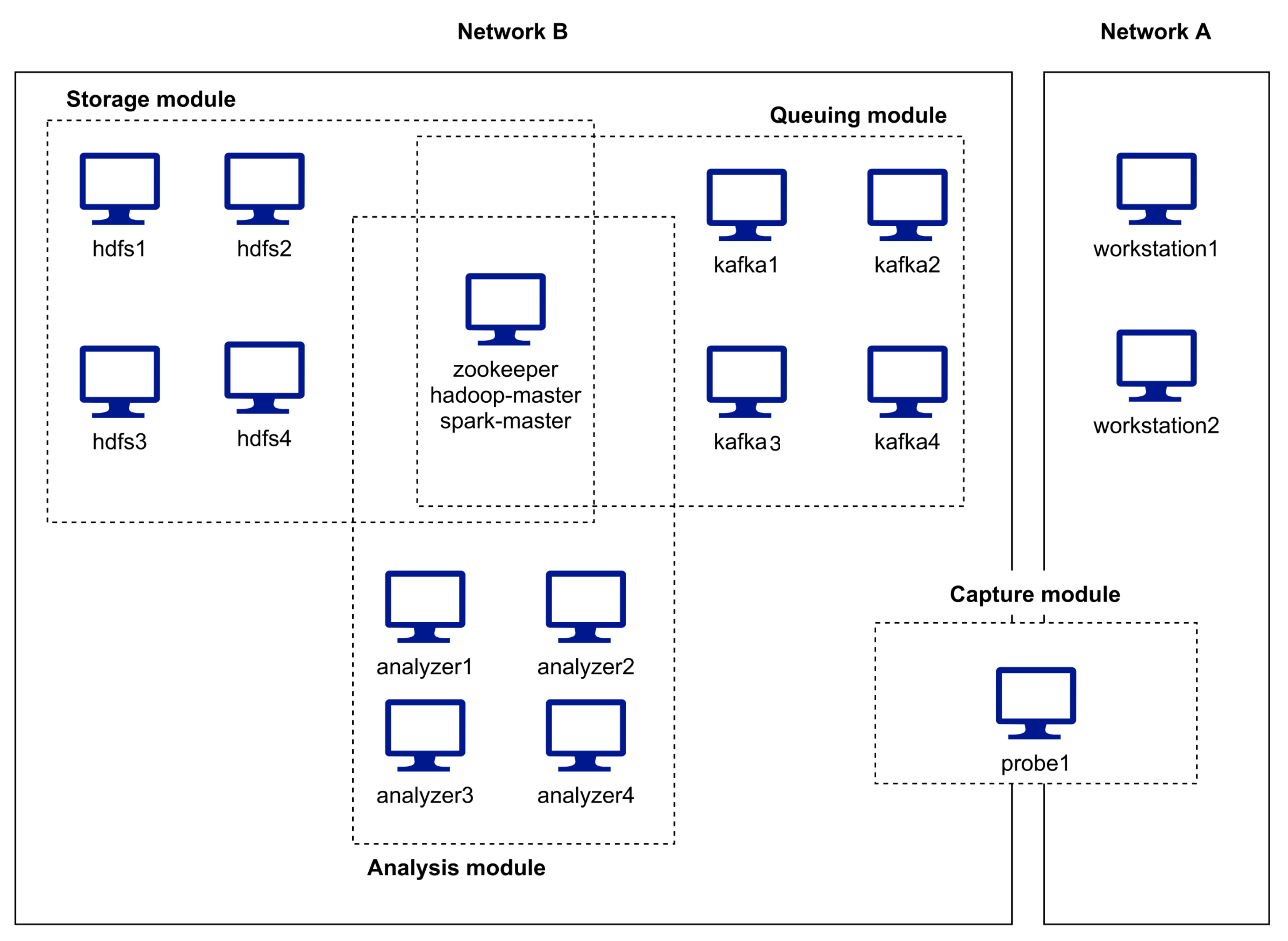
The testbed used for the evaluation is represented in Figure 3. It includes 16 hosts and involves two different networks (A and B). The hosts that support the IDS modules operate on network B. Two systems, whose traffic exchanged is meant to be captured by a probe, operate on network A. The probe is thus a multi-homed host, once it captures traffic passing by in network A, which it then forwards to the queuing nodes in network B.

Network A runs at 1 Gbps and is built on a Cisco Catalyst 2960-S switch, while Network B is built on a 10 Gbps Cisco Nexus 93108TC-EX switch. A 1 Gbps link connects both switches. The probe connects only to the Network A switch, using two different ports: one is used as a destination, via port mirroring, of all traffic exchanged by the workstations; the other is used for the traffic outgoing to network B, which will still need to pass through the link between the two switches. Network A and Network B both operate with the same default MTU (1500 bytes). However, in each network, hosts operate in different Virtual LANs.

The hosts in network A are physical hosts, all running Linux (Ubuntu Server 20.04.3 LTS). The traffic generators (workstations) are off-the-shelf PCs (with an Intel 6-core i7-8700 CPU operating at 3.2/4.6Ghz, 16 GB of RAM, 460 GB SATA III SSD, on-board Intel I219-V 1 Gbps Ethernet NIC). The probe host is a system of the same class, although with slightly different hardware characteristics (Intel 4-core i7-920 CPU operating at 2.67/2.93 Ghz, 24 GB of RAM, 240 GB SATA III SSD, two on-board Realtelk 8111C 1 Gbps Ethernet NICs).

The hosts that support the queuing, storage, analysis and coordination functions are all Linux (Debian 11) Virtual Machines (VMs), running in a Proxmox VE 7 virtualization cluster. Each cluster node has 2 AMD EPYC 7351 16-core CPUs, 256 GB of RAM and NVMe (PCIe 3) SSD storage. The characteristics of the virtual machines used are shown in

Table 1. Virtual hardware of the services hosts.

Service	#VMs	vCores per VM	vRAM per VM (GiB)	vDisk per VM (GB)
Kafka	4	4	16	96
HDFS	4	4	8	128
Spark 1	2	4	64	32
Spark 2	1	4	64	96
Spark 3	1	4	64	64
Spark 4	1	4	64	32
Zookeeper	1	4	8	16

:

To reach the dimensions laid out in Table 1, some calculations were performed considering the following requirements: $R_1$) to be able to capture full packets at 1 Gbps line rate, for 10 min; $R_2$) to be able to perform two captures simultaneously ($\#KafkaCaptures$ = 2) while keeping one replica for each capture ($\#KafkaReplicas$ = 1) in the Kafka nodes; $R_3$) to be able to keep three different captures stored ($\#PersistentCaptures$ = 3), with one replica each ($\#PersistentReplicas$ = 1), in the HDFS nodes.

To begin with, requirement $R_1$ generates a file per capture with an overall size $SizeOfCapture$ = 75 GB. This, together with requirement $R_2$ implies that the amount of secondary storage needed per Kafka node (VM) is given by

$$\frac{SizeOfCapture\times \#KafkaCaptures\times (\#KafkaReplicas+1)}{\#KafkaNodes}+SizeoOfOS,$$

(1)

where $\#KafkaNodes$ is the number of Kafka nodes and $SizeoOfOS$ is the amount of storage reserved, in all nodes, for the Operating System (OS). As in this testbed $\#KafkaNodes$ = 4 and $SizeOfOS$ = 15 GB, then each Kafka node will need at least 90 GB of secondary storage; this was further rounded up to the nearest multiple of 16 GB (96 GB in this case), thus providing some extra storage space to avoid operating with too tight constraints (the same rationale was applied to the virtual disks of the other testbed VMs).

By requirement $R_3$, the secondary storage needed by each HDFS node is given by

$$\frac{SizeOfCapture\times \#PersistentCaptures\times (\#PersistentReplicas+1)}{\#HDFSNodes}+SizeOfOS,$$

(2)

where $\#HDFSNodes$ is the number of HDFS nodes, which is 4 in the testbed. Thus, each HDFS node needs 112.5 GB of disk space, further rounded up to 128 GB.

With regard to the Spark nodes, the testbed uses four VMs of three different types: two VMs are of the type Spark1, one is of the type Spark2 and another is of the type Spark3. Each type requires a different amount of storage: Spark1 VMs only perform operations in memory and so, in addition to the disk space needed for the OS (15 GB), a similar extra amount was assigned to ensure a comfortable operation, totaling 32 GB of virtual disk; in addition to the OS, the Spark2 VM also holds a full capture (75 GB), thus requiring 96 GB of storage; finally, besides the OS, the Spark3 VM only holds half a capture (37.5 GB), and so it ends up needing only 64 GB of virtual disk.

The Apache Zookeeper service, the Apache Hadoop NameNode and the Apache Spark master service, are all running on the same virtual machine, since their coordination roles do not require much computational resources. In a real scenario, these services should operate on separate hosts and with more than one instance for fault-tolerance reasons.

3.2. Methodology

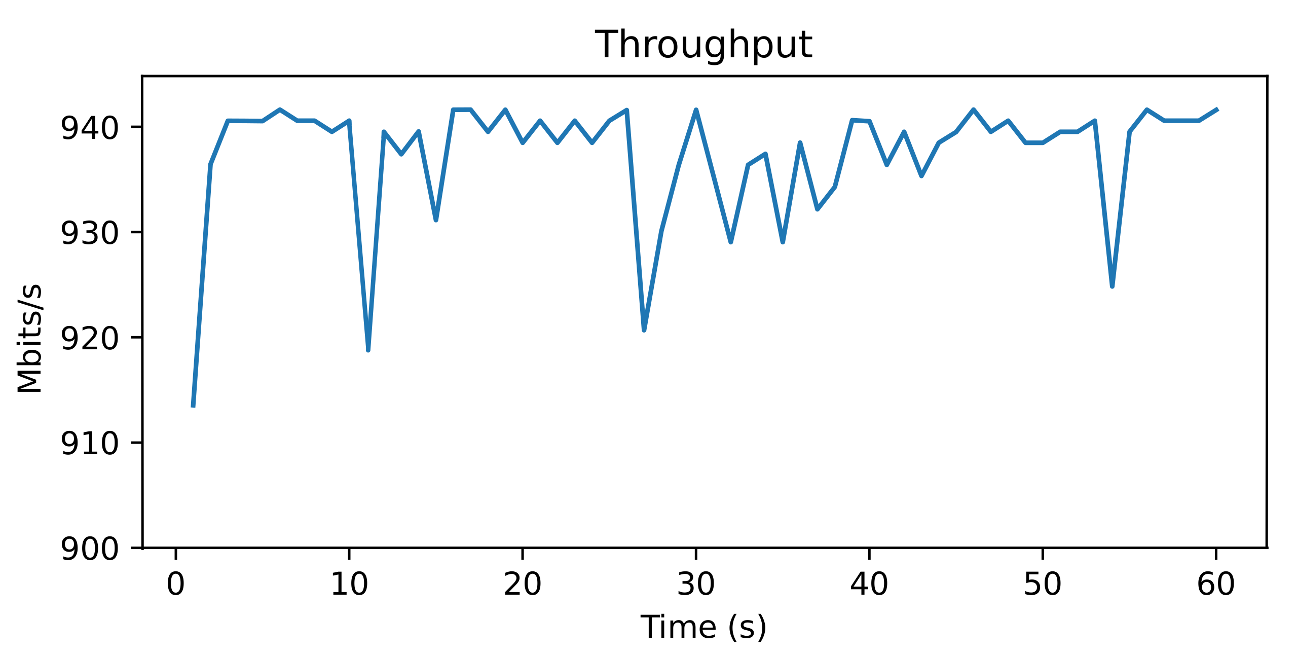
Due to the characteristics of the testbed, the network captures on Network A were limited to a nominal maximum of 1 Gbps. However, before beginning the evaluation of the architecture, a test was made to verify what was the effective maximum bandwidth achievable between the workstations. The test consisted of running the iPerf3 [41] benchmark for 60 s, to measure the bandwidth of a single TCP connection between the workstations. The actual throughput can be found in Figure 4, with most values sitting between 930 and 940 Mbps. These values set a ceiling for the expected probe capture rate.

Depending on the specific scenario, two different types of network captures were performed: full-packet captures or headers-only (truncated) captures. In the first type, each network packet is captured as is (minus the layer 1 of the OSI model), whereas in the second type only the headers are captured (and the OSI layer 1 is also not captured).

In the following experiments, the headers-only capture has the packets truncated at 96 bytes, allowing to acquire the data link, network and transport layers, and also some bytes of the payload, which permits to collect some intel regarding the network activity. Also, every network transaction in Network B was secured by SSL, unless stated otherwise.

Each experiment, involving a specific combination of parameters, was repeated five times. The relevant metrics for each of the five runs are shown, as well as their average value and corresponding standard deviation (allowing to assess the stability of the prototype).

There are two base parameters regarding the packet flow on all experiments (except the one from Section 4.4): one is the duration of the capture (60 or 300 s) and the other is the size of the captured packets (full-packets or headers-only packets truncated at 96 bytes).

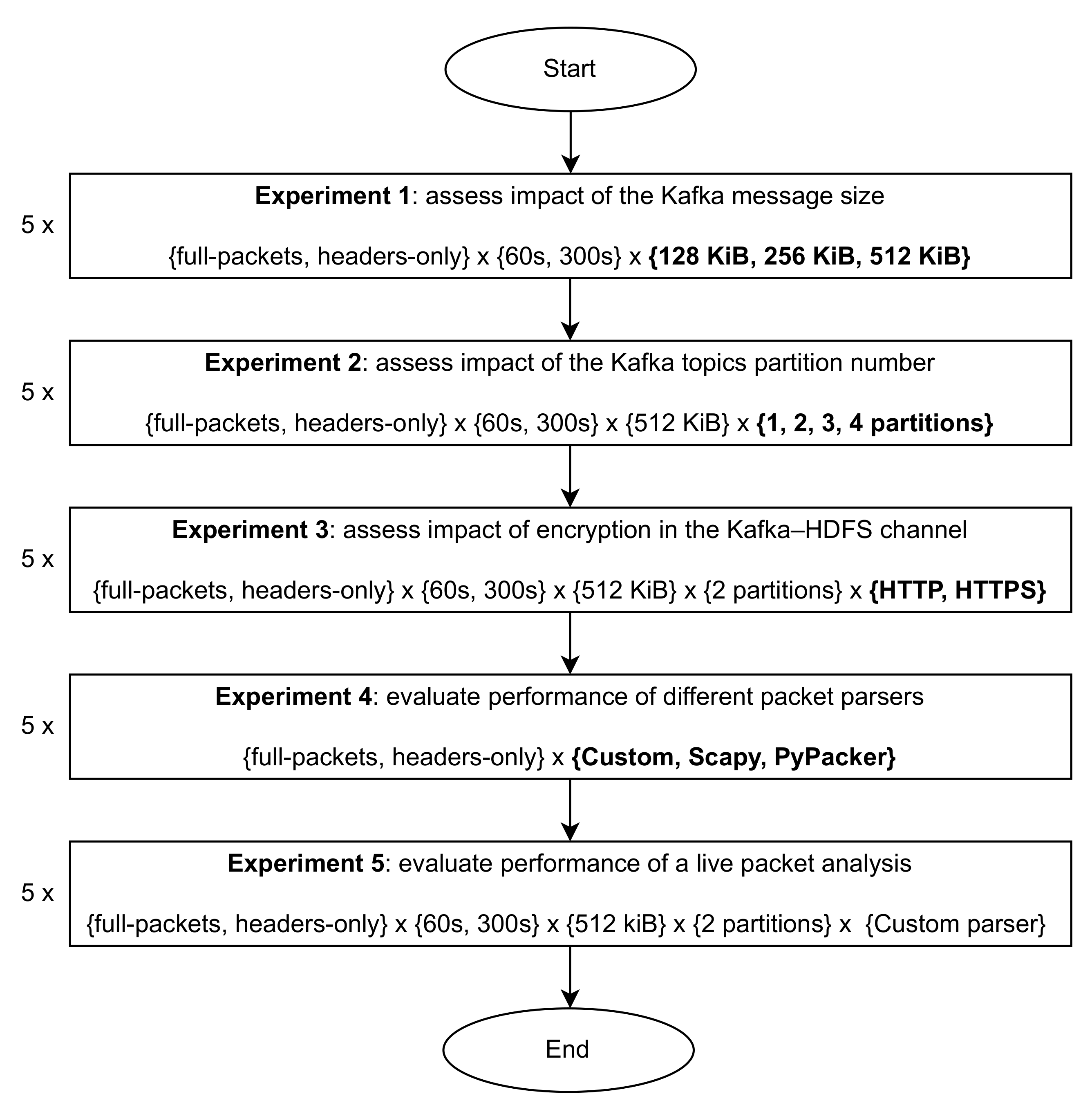
Several experiments were thus performed, in the following order:

• Study the impact of the message size for the messages published on the queuing module (Section 4.1). A specific size will be selected to be used on the remaining tests.
• Assess the effect of a different number of partitions for a topic in the Kafka cluster (Section 4.2). There are four Kafka nodes, meaning a topic can have up to four partitions (one per node). A specific number of partitions will be selected to be used thereafter.
• Investigate the repercussions of using or not encryption (HTTPS vs HTTP) when storing the network captures in the HDFS cluster (Section 4.3). Depending on the deployment scenario of our IDS, encrypting the Kafka–HDFS channel may or may not be necessary, and so it is important to understand the performance trade-offs involved.
• As this IDS also performs packet analysis, it is necessary to find the fastest packet parser, which will be the core of the analysis applications. To this extent, three different parsers are compared (Section 4.4) and one is selected to be used in the last experiment.
• Assess the IDS in the context of a live (online) packet analysis (Section 4.5).

The experimental methodology followed to evaluate our IDS protytpe is summarized in Figure 5. In each experiment, different parameter combinations are tested (each combination is tested five times). Also, some experiments adopt specific values for certain parameters, depending on the conclusions drawn in the previous experiments; this is the case for the adoption of a message size of 512 KB after Experiment 1, two topic partitions after Experiment 2, and the use of our custom parser after Experiment 4—see Section 4 for details.

4. Experimental Results and Discussion

This section presents the detailed results of the experiments in the stipulated order.

4.1. Impact of the Kafka Message Size

(Near) Real-time network captures are very time-sensitive and so they must be as optimized as possible. In this experiment the goal is to find the Apache Kafka message size that minimizes the data streaming time, that is, the time spent in publishing and consuming the network captures. Apache Kafka was not designed to handle large-size messages, not being recommended to produce messages above 1 Megabyte (MB). Therefore, only the following messages sizes were tested (all bellow the 1 MB limit and up to half of that value):

• 128 KB ($2^{17}$ or 131,072 bytes) ;
• 256 KB ($2^{18}$ or 262,144 bytes);
• 512 KB ($2^{19}$ or 524,288 bytes).

The outputs (metrics collected) of the experiment are an upload delay, a download delay and a total delay (sum of the upload and download delays), all measured in seconds. The upload delay is the time elapsed between the capture of the last network packet and its publication on Kafka. The download delay is the time elapsed between the moment in which the last message was uploaded on Kafka and its consumption by a Spark consumer.

This experiment was executed on a Kafka topic with two partitions and one replica, thus using two of the Kafka VMs (one per partition) available in the testbed. Also, only one Spark VM (Spark 4 configuration) was used, and none HDFS VMs were involved.

Table 2. Kafka delays on a 60 s full-packet capture, for different message sizes. (*) Denotes best value.

Kafka Message Size (KB)	Run	Upload Delay (s)	Download Delay (s)	Total Delay (s)	Packet Loss (%)
128	1	107.97	3.38	111.35	0.005
	2	92.91	14.48	107.39	0.027
	3	84.52	19.00	103.52	0.003
	4	91.95	14.98	106.93	0.005
	5	97.25	11.09	108.34	0
	AVG	94.92	12.59	107.51	0.008
	SD	7.7 (8.11%)	5.24 (41.64%)	2.52 (2.34%)	0.010
256	1	85.75	31.10	116.85	0
	2	97.98	16.56	114.54	0.011
	3	92.09	30.26	122.35	0.012
	4	93.45	26.11	119.57	0.034
	5	93.67	31.67	125.34	0.002
	AVG	93.45	30.26	119.57	0.011
	SD	3.95 (4.23%)	5.64 (18.63%)	3.84 (3.21%)	0.012
512	1	85.14	4.33	89.47	0
	2	79.38	4.62	84.01	0.001
	3	89.21	1.04	90.25	0.020
	4	73.60	4.23	77.83	0
	5	86.80	6.15	92.94	0.004
	AVG	85.14	4.33	89.47 (*)	0.001
	SD	5.64 (6.62%)	1.67 (38.51%)	5.38 (6.02%)	0.008

and

Table 3. Kafka delays on a 60 s headers-only capture, for different message sizes.

Kafka Message Size (KB)	Run	Upload Delay (s)	Download Delay (s)	Total Delay (s)	Packet Loss (%)
128	1	0.94	1.02	1.95	0
	2	0.83	1.01	1.84	0
	3	0.08	1.01	1.09	0
	4	0.22	1.01	1.23	0
	5	0.59	1.01	1.60	0
	AVG	0.53	1.01	1.54	0
	SD	0.33 (63.18%)	0 (0.27%)	0.34 (21.77%)	0
256	1	0.97	1.02	1.99	0
	2	0.59	1.01	1.60	0
	3	0.76	1.01	1.77	0
	4	0.85	1.01	1.86	0
	5	0.66	1.01	1.67	0
	AVG	0.76	1.01	1.77	0
	SD	0.13 (17.62%)	0 (0.39%)	0.14 (7.71%)	0
512	1	0.57	1.02	1.58	0
	2	0.22	1.01	1.23	0
	3	0.54	1.01	1.55	0
	4	0.98	1.01	1.99	0
	5	0.72	1.01	1.73	0
	AVG	0.57	1.01	1.58	0
	SD	0.25 (43.86%)	0 (0.42%)	0.25 (15.68%)	0

show the results of the full-packet and headers-only captures during 60 s, and

Table 4. Kafka delays on a 300 s full-packet capture, for different message sizes. (*) Denotes best value.

Kafka Message Size (KB)	Run	Upload Delay (s)	Download Delay (s)	Total Delay (s)	Packet Loss (%)
128	1	513.76	30.19	543.94	0.002
	2	408.36	70.46	478.82	0.002
	3	420.17	72.48	492.64	0.002
	4	445.22	78.70	523.92	0.004
	5	395.45	61.42	456.86	0.004
	AVG	436.59	62.65	499.24	0.003
	SD	41.92 (9.6%)	17.15 (27.4%)	31.19 (6.25%)	0.001
256	1	411.74	204.90	616.63	0.005
	2	395.83	198.02	593.84	0.005
	3	417.88	199.52	617.40	0.001
	4	423.74	158.09	581.83	0.006
	5	421.18	191.13	612.31	0.006
	AVG	417.88	198.02	612.31	0.005
	SD	9.97 (2.39%)	16.71 (8.44%)	14.16 (2.31%)	0.002
512	1	426.03	1.71	427.74	0.001
	2	422.27	1.92	424.19	0.006
	3	455.18	1.03	456.21	0.001
	4	457.94	1.04	458.99	0.002
	5	459.52	1.04	460.56	0.002
	AVG	455.18	1.04	456.21 (*)	0.002
	SD	16.47 (3.62%)	0.39 (37.2%)	16.08 (3.52%)	0.002

and

Table 5. Kafka delays on a 300 s headers-only capture, for different message sizes.

Kafka Message Size (KB)	Run	Upload Delay (s)	Download Delay (s)	Total Delay (s)	Packet Loss (%)
128	1	0.82	0.62	1.44	0
	2	0.12	1.01	1.13	0
	3	0.35	1.01	1.36	0
	4	0.45	1.01	1.46	0
	5	0.41	1.04	1.45	0
	AVG	0.43	0.94	1.37	0
	SD	0.23 (52.8%)	0.16 (16.95%)	0.12 (9.09%)	0
256	1	1.05	1.01	2.06	0
	2	0.87	1.01	1.88	0
	3	0.83	1.01	1.83	0
	4	0.29	1.00	1.29	0
	5	0.38	1.00	1.38	0
	AVG	0.83	1.01	1.83	0
	SD	0.29 (35.73%)	0 (0.35%)	0.3 (16.26%)	0
512	1	0.47	1.01	1.48	0
	2	0.55	1.00	1.56	0
	3	0.39	1.00	1.40	0
	4	0.62	1.00	1.62	0
	5	0.45	1.00	1.46	0
	AVG	0.47	1.00	1.48	0
	SD	0.08 (16.57%)	0 (0.08%)	0.08 (5.32%)	0

show the same type of results for a 300 s capture.

Looking at the results, the message size that minimizes the total delay for full-packet captures is consistently 512 KB (see (*) on Table 2 and Table 4). For truncated captures, the best message size under the same criteria is 128 KB, but closely followed by 512 KB which, in turn, exhibits a smaller standard deviation, thus having a more predictable behavior. Moreover, once all the delays for truncated captures are very small (in comparison to full captures), making their differences also very small (even if the relative standard deviations tend to be higher), then a best message size of 512 KB can be generalized both for full and truncated captures, and this is the message size assumed henceforth in the next experiments.

The fact that the delays for headers-only captures are very small means that the system does not throttle while capturing truncated network packets, allowing its operation for an unlimited time in such regime, as long it has enough disk space to store the captured data. Or, if the system performs only the analysis of the data (without storing it), it may operate forever (depending on the core parser performance—see Section 4.5).

On the other hand, for full-packet captures, the delays are much higher (up to two orders of magnitude) and seem to increase in direct proportion of the capture duration (e.g., going from a 1 min to a 5 min capture increases the delay roughly five times, for any message size). Therefore, having the publishing delay increasing along the time of operation makes it impossible to perform a real-time network traffic capture and analysis, even if such data is not stored in persistent storage (which would add a further delay).

It should also be noticed that the packet loss for full captures is very low, and totally absent for truncated captures, regardless of the capture duration.

4.2. Impact of the Kafka Topics Partition Number

When creating a Kafka topic it is necessary to define the number of partitions for that topic (in the previous experiment, that number was two). The partitions may be distributed across Kafka nodes or placed on the same host. It is up to Kafka to decide which host will be responsible for which partitions, though prioritizing the ones holding fewer partitions, but how many partitions should a topic have to ensure the best performance?

In principle, more partitions should benefit performance (for load balance reasons), but the extra effort involved (communication and coordination) may not pay off. In order to answer such a question conclusively for our testbed, further experiments were conducted, whereby the number of partitions varied from one to four, with each partition assigned to a separate Kafka node (and so the number of Kafka nodes used varied accordingly). As before, only the Spark 4 VM was used, and no HDFS VMs were involved in the experiment.

Table 6. Kafka delays on a 60 s full-packet capture, for different numbers of topic partitions. (*) Denotes best value.

Number of Kafka Partitions	Run	Upload Delay (s)	Download Delay (s)	Total Delay (s)	Packet Loss (%)
1	1	209.17	10.92	220.09	0.0112
	2	227.31	1.03	228.34	0
	3	201.25	10.97	212.22	0.0217
	4	218.96	4.16	223.12	0.0327
	5	200.50	15.37	215.87	0.0619
	AVG	211.44	8.49	219.93	0.0255
	SD	10.36 (4.9%)	5.17 (60.93%)	5.6 (2.55%)	0.0212
2	1	91.40	1.02	92.42	0.0025
	2	87.91	2.47	90.38	0.0430
	3	89.75	2.21	91.97	0
	4	85.58	4.64	90.21	0.0190
	5	95.36	1.03	96.39	0.0187
	AVG	89.75	2.21	91.97	0.0187
	SD	3.31 (3.68%)	1.32 (59.68%)	2.23 (2.43%)	0.0153
3	1	43.67	1.27	44.94	0.0206
	2	45.90	1.02	46.93	0.0040
	3	43.97	1.08	45.05	0.0417
	4	40.39	1.22	41.61	0.0072
	5	43.48	1.89	45.37	0.0394
	AVG	43.67	1.22	45.05	0.0206
	SD	1.77 (4.06%)	0.31 (25.45%)	1.74 (3.86%)	0.0157
4	1	15.34	8.03	23.38	0.0298
	2	14.43	6.56	20.99	0.0247
	3	15.11	8.52	23.63	0.0405
	4	15.44	6.12	21.56	0.0157
	5	13.45	8.35	21.80	0.0681
	AVG	15.11	8.03	21.80 (*)	0.0298
	SD	0.74 (4.9%)	0.98 (12.23%)	1.04 (4.79%)	0.0181

and

Table 7. Kafka delays on a 60 s headers-only capture, for different numbers of topic partitions.

Number of Kafka Partitions	Run	Upload Delay (s)	Download Delay (s)	Total Delay (s)	Packet Loss (%)
1	1	0.41	0.96	1.37	0
	2	0.31	0.96	1.27	0
	3	0.59	0.95	1.55	0
	4	0.67	0.95	1.63	0
	5	0.56	0.95	1.51	0
	AVG	0.51	0.96	1.46	0
	SD	0.13 (25.85%)	0 (0.3%)	0.13 (8.81%)	0
2	1	0.81	0.96	1.77	0
	2	0.97	0.97	1.93	0
	3	0.34	0.97	1.32	0
	4	0.55	0.98	1.53	0
	5	0.23	0.98	1.21	0
	AVG	0.55	0.97	1.53	0
	SD	0.28 (50.42%)	0.01 (0.59%)	0.27 (17.84%)	0
3	1	0.87	0.98	1.85	0
	2	0.04	0.98	1.03	0
	3	0.38	0.99	1.36	0
	4	0.31	0.98	1.30	0
	5	0.17	0.99	1.15	0
	AVG	0.31	0.98	1.30	0
	SD	0.28 (91.09%)	0 (0.17%)	0.28 (21.81%)	0
4	1	0.45	0.98	1.44	0
	2	0.33	0.98	1.31	0
	3	0.59	0.98	1.57	0
	4	0.69	0.98	1.67	0
	5	0.25	0.99	1.23	0
	AVG	0.45	0.98	1.44	0
	SD	0.16 (35.74%)	0 (0.15%)	0.16 (11.2%)	0

show the results of the full-packet and headers-only captures during 60 s, and

Table 8. Kafka delays on a 300 s full-packet capture, for different numbers of topic partitions. (*) Denotes best value.

Number of Kafka Partitions	Run	Upload Delay (s)	Download Delay (s)	Total Delay (s)	Packet Loss (%)
1	1	1072.03	9.44	1081.46	0.0013
	2	1182.27	1.04	1183.31	0.0024
	3	1180.52	1.03	1181.55	0.0024
	4	1016.93	49.78	1066.72	0.0013
	5	1213.38	1.04	1214.42	0.0112
	AVG	1133.03	12.47	1145.49	0.0037
	SD	75.28 (6.64%)	18.9 (151.9%)	59.64 (5.21%)	0.0038
2	1	445.88	2.24	448.11	0.0075
	2	423.89	1.09	424.98	0.0004
	3	460.77	1.41	462.19	0
	4	461.88	1.03	462.90	0.0035
	5	439.50	1.88	441.38	0.0158
	AVG	445.88	1.41	448.11	0.0035
	SD	14.15 (3.17%)	0.47 (33.05%)	14.12 (3.15%)	0.0058
3	1	228.70	1.03	229.73	0.0155
	2	231.44	1.02	232.47	0.0002
	3	227.52	1.30	228.82	0.0102
	4	222.79	1.05	223.84	0.0099
	5	222.99	1.16	224.15	0.0067
	AVG	227.52	1.05	228.82	0.0099
	SD	3.35 (1.47%)	0.11 (10.18%)	3.33 (1.46%)	0.0050
4	1	104.14	1.03	105.17	0.0053
	2	103.20	1.03	104.24	0.0145
	3	103.97	1.42	105.39	0.0039
	4	110.97	1.14	112.11	0.0082
	5	98.66	1.34	100.00	0.0133
	AVG	103.97	1.14	105.17 (*)	0.0082
	SD	3.94 (3.79%)	0.16 (14.12%)	3.89 (3.7%)	0.0042

and

Table 9. Kafka delays on a 300 s headers-only capture, for different numbers of topic partitions.

Number of Kafka Partitions	Run	Upload Delay (s)	Download Delay (s)	Total Delay (s)	Packet Loss (%)
1	1	0.11	1.01	1.12	0
	2	0.13	1.01	1.14	0
	3	0.28	1.01	1.29	0
	4	0.86	1.01	1.86	0
	5	0.85	1.01	1.86	0
	AVG	0.45	1.01	1.45	0
	SD	0.34 (75.79%)	0 (0.05%)	0.34 (23.28%)	0
2	1	0.12	1.00	1.13	0
	2	0.38	1.01	1.39	0
	3	0.78	1.01	1.79	0
	4	0.66	1.01	1.67	0
	5	0.23	1.01	1.23	0
	AVG	0.38	1.01	1.39	0
	SD	0.25 (67.32%)	0 (0.18%)	0.25 (18.28%)	0
3	1	0.54	1.01	1.55	0
	2	0.25	1.02	1.27	0
	3	0.01	1.01	1.02	0
	4	0.13	1.01	1.15	0
	5	0.33	1.01	1.34	0
	AVG	0.25	1.01	1.27	0
	SD	0.18 (71.99%)	0 (0.22%)	0.18 (14.29%)	0
4	1	0.67	1.02	1.69	0
	2	0.52	1.01	1.54	0
	3	0.59	1.01	1.60	0
	4	0.41	1.01	1.42	0
	5	0.88	1.01	1.89	0
	AVG	0.59	1.01	1.60	0
	SD	0.16 (26.69%)	0 (0.34%)	0.16 (9.9%)	0

show the same results for a 300 s capture. The metrics collected (upload delay, download delay, total delay, and packet loss) are the same, and have the same meaning, as those collected in the experiment of the previous section.

For full captures the results leave no doubt: it is surely better, performance-wise, to use more topic partitions; in fact, increasing the number of partitions by one unit makes the total delay to be roughly halved. However, for truncated captures, the results are somewhat inconclusive, once there are no significant differences in the overall Kafka delay (it is true that three partitions ensure the absolute lowest delays, but by a small margin). Again, there is no packet loss for the truncated captures, and the loss is negligible for full captures.

All things considered, this seems to point to the general conclusion that more partitions ensures better performance (or, at least, do not impair it), and having a single partition per Kafka node should yield a good load balance. However, more partitions may not be feasible, or even justifiable, in a real scenario. For instance, the possible number of Kafka nodes may be too small, thus limiting Kafka’s scalability. Or, as it happens in our IDS prototype, real-time (or even near real-time) assessment of full-packet captures is currently not possible, even with four partitions, and so there is no need to fully use them in a single capture, as they may be used on other captures that are being performed at the same time. For this reason, the number of partitions will be kept at two for the remaining experiments.

Also note that the partition configuration depends on the specific target scenario. Our IDS is flexible enough to accommodate multiple Kafka topics with different numbers of partitions and such is completely transparent to the consumers and producers (they will always work with all the partitions that are assigned to a specific topic).

4.3. Impact of Encryption in the Kafka–HDFS Channel

The goal of this experiment is to assess the IDS performance when capturing and storing data persistently into the HDFS cluster, using either clear-text or TLS encryption for the communication between the Kafka and the HDFS components. By default, communications between all testbed components are TLS-encrypted. However, depending on the IDS deployment scenario (e.g., private/public/cloud-based network), the privacy requirements may vary. For instance, it is expected that the communication channel between Kafka and HDFS sits on a private network, whereas Kafka may be exposed in a public network in order to be feed with public captures. Therefore, it is important to gain insight on the possible performance gains of removing encryption wherever such is deemed as safe.

The experiment was executed with a Kafka topic with two partitions and, as in the previous tests, the messages were published to Kafka in chunks of 512 KB. For this specific experiment, two HDFS nodes were made available and the replication level was set to two, meaning any file placed in HDFS is replicated in the two nodes.

The metrics collected are similar to the ones collected in the experiments of the previous two sections, but with the download delay now representing the time elapsed between the publication of the last message on Kafka and its storage on the HDFS cluster.

The results of the experiment may be seen in

Table 10. HDFS delays on a 60 s full-packet capture, when using HTTP vs. HTTPS. (*) Denotes best value.

Protocol	Run	Upload Delay (s)	Download Delay (s)	Total Delay (s)	Packet Loss (%)
HTTP	1	105.11	1.25	106.36	0
	2	98.70	1.06	99.76	0
	3	88.86	1.44	90.31	0.0351
	4	94.92	1.44	96.36	0.0294
	5	88.33	1.91	90.24	0
	AVG	95.19	1.42	96.61 (*)	0.0129
	SD	6.29 (6.61%)	0.28 (19.91%)	6.09 (6.3%)	0.0159
HTTPs	1	83.83	151.23	235.06	0.0021
	2	106.79	127.35	234.15	0.0556
	3	97.26	135.53	232.78	0
	4	89.73	148.42	238.15	0.0066
	5	102.02	135.04	237.05	0
	AVG	97.26	135.53	235.06	0.0021
	SD	8.27 (8.5%)	8.95 (6.6%)	1.94 (0.83%)	0.0215

and

Table 11. HDFS delays on a 60 s headers-only capture, when using HTTP vs. HTTPS.

Protocol	Run	Upload Delay (s)	Download Delay (s)	Total Delay (s)	Packet Loss (%)
HTTP	1	0.48	1.03	1.51	0
	2	0.92	1.03	1.95	0
	3	0.78	1.03	1.81	0
	4	0.65	1.03	1.68	0
	5	0.76	1.02	1.78	0
	AVG	0.72	1.03	1.75	0
	SD	0.15 (20.38%)	0 (0.3%)	0.14 (8.29%)	0
HTTPs	1	0.49	1.03	1.52	0
	2	0.73	1.02	1.75	0
	3	0.45	1.02	1.47	0
	4	0.98	1.01	2.00	0
	5	0.71	1.03	1.73	0
	AVG	0.71	1.02	1.73	0
	SD	0.19 (27.06%)	0.01 (0.5%)	0.19 (10.83%)	0

(60 s capture), and

Table 12. HDFS delays on a 300 s full-packet capture, when using HTTP vs. HTTPS. (*) Denotes best value.

Protocol	Run	Upload Delay (s)	Download Delay (s)	Total Delay (s)	Packet Loss (%)
HTTP	1	447.13	1.04	448.18	0.0053
	2	486.93	1.03	487.97	0.0083
	3	478.82	1.39	480.20	0.0112
	4	441.63	1.27	442.90	0.0075
	5	491.01	1.23	492.24	0.0051
	AVG	469.11	1.19	470.30 (*)	0.0075
	SD	20.64 (4.4%)	0.14 (11.38%)	20.65 (4.39%)	0.0022
HTTPs	1	454.57	724.28	1178.85	0.0086
	2	457.93	708.41	1166.33	0.0021
	3	481.08	651.90	1132.98	0.0049
	4	454.69	699.53	1154.22	0.0089
	5	462.68	711.80	1174.48	0.0061
	AVG	457.93	708.41	1166.33	0.0061
	SD	9.9 (2.16%)	24.94 (3.52%)	16.49 (1.41%)	0.0025

and

Table 13. HDFS delays on a 300 s headers-only capture, when using HTTP vs. HTTPS.

Protocol	Run	Upload Delay (s)	Download Delay (s)	Total Delay (s)	Packet Loss (%)
HTTP	1	0.35	1.03	1.38	0
	2	0.77	1.02	1.79	0
	3	0.82	1.03	1.84	0
	4	0.40	1.02	1.42	0
	5	0.94	1.02	1.96	0
	AVG	0.66	1.02	1.68	0
	SD	0.24 (35.9%)	0 (0.16%)	0.24 (14.01%)	0
HTTPs	1	0.07	1.03	1.10	0
	2	0.54	1.01	1.55	0
	3	0.09	1.02	1.11	0
	4	0.15	1.02	1.17	0
	5	0.75	1.03	1.78	0
	AVG	0.15	1.02	1.17	0
	SD	0.28 (185.6%)	0.01 (0.69%)	0.28 (23.65%)	0

(300 s capture), for both full-packet and truncated captures.

The conclusion is somehow expected. For truncated captures (with very small amounts of network data involved) it makes little or no difference to use HTTPS (the fact that, during the 300 s capture, using HTTPS ended up being faster than using HTTP, should not be prone to any generalization, once the delays at stake are very small and thus very susceptible to even small fluctuations, as hinted by the higher relative standard deviations).

However, for full captures, using HTTPS makes the total delay become more than twice (roughly 2.5 times) of that delay when using HTTP, regardless of the capture duration. The specific reason for this increase lies in the download delay (HDFS insertion), which increases approximately 100 times for the 60 s capture, and near 700 times for the 300 s capture, while the upload delay remains essentially the same whether HTTPS or HTTP is used. Therefore, it is very advantageous, performance-wise, to have an IDS deployment that dispense with communications encryption. This, of course, requires an isolated environment for the IDS services and some degree of administrative access to the underlying platforms (network and compute), in order to ensure a secure execution.

Still concerning full captures, another observation that deserves to be highlighted is that, as already verified in the experiment of Section 4.1, the total delays increase in direct proportion of the duration of the captures, that is, during a 300 s capture, the delays are roughly five times higher than those observed during a 60 s capture, whether HTTP or HTTPS is used. This reinforces the statement already made in Section 4.1, whereby it was assumed that, currently, our IDS cannot sustain continuous (or even medium duration) captures.

For the packet loss, the same scenario of the previous experiments was again observed (no packet loss for truncated captures, and negligible for full-captures).

4.4. Performance of Different Core Parsers

In our IDS, every analysis application includes a core parser. Its function is to obtain the raw data from a Kafka topic and extract the relevant information for the analysis.

The raw data is processed message by message. When the analyzer receives a message (chunk) from Kafka, it extracts the packet header to know the exact length of the network packet, and then retrieves the full packet. Right after, the core parser analyses the packet, layer by layer. Since the network packets are captured from the Ethernet layer (OSI Layer 2), the parser knows how to start the extraction process. It reads which protocol is in the next layer; this way, it can extract the information accordingly to the protocol specification (available on RFC documents). After it finishes extracting the information of the packet, the parser will advance to the next packet, until it reaches the end of the chunk; when that happens, it will fetch another chunk (if available); otherwise, it will wait for new data.

In this work, three options for the core parser were considered: two community tools (Scapy [42] and PyPacker [43]), and a custom parser specifically crafted for our IDS. The later was developed as a simple alternative, meant to be faster, once it only parses the necessary data for a specific analysis, while Scapy and PyPacker perform a full parsing.

In order to highlight the performance of the custom parser, an experiment was conducted with the three parsers to evaluate their peak performance. Thus, the experiment was performed in offline mode, parsing data from PCAP files instead of a live Kafka stream. Two PCAP files were parsed, both with a total size of 10 GB. One of the files—file A—contains a full-packet capture carrying 5,708,800 packets. The other file—file B—contains a headers-only (packets truncated at 96 bytes) packet capture carrying 102,152,015 packets.

For each run of the experiment, the total execution time (parsing time) was registered and the number of packets processed per second (parsing rate) was calculated.

Table 14. Core parsers peak-performance for the offline analysis of full packets (file A). (*) Denotes best value.

Parser	Run	Parsing Time (s)	Parsing Rate (Packets/s)
Custom	1	53.87	105,978
	2	54.23	105,265
	3	55.93	102,067
	4	56.23	101,520
	5	56.44	101,153
	AVG	55.34 (*)	103,197 (*)
	SD	1.07 (1.94%)	2013.65 (1.95%)
Scapy	1	1487.11	3839
	2	1502.62	3799
	3	1507.96	3786
	4	1528.63	3735
	5	1508.52	3784
	AVG	1507.96	3786
	SD	13.31 (0.88%)	33.41 (0.88%)
PyPacker	1	255.58	22,336
	2	257.41	22,178
	3	256.67	22,242
	4	254.14	22,464
	5	255.61	22,334
	AVG	255.61	22,334
	SD	1.11 (0.43%)	96.87 (0.43%)

and

Table 15. Core parsers peak-performance for the offline analysis of truncated packets (file B). (*) Denotes best value.

Parser	Run	Parsing Time (s)	Parsing Rate (Packets/s)
Custom	1	823.07	124,111
	2	810.13	126,093
	3	818.60	124,789
	4	830.69	122,973
	5	801.89	127,389
	AVG	816.88 (*)	125,071 (*)
	SD	10.02 (1.23%)	1537.61 (1.23%)
Scapy	1	26,073.21	3918
	2	25,909.96	3943
	3	26,310.25	3883
	4	26,126.60	3910
	5	25,798.62	3960
	AVG	26,073.21	3918
	SD	177.06 (0.68%)	26.65 (0.68%)
PyPacker	1	4266.07	23,945
	2	4250.54	24,033
	3	4200.30	24,320
	4	4312.05	23,690
	5	4264.74	23,953
	AVG	4264.74	23,953
	SD	35.82 (0.84%)	202.12 (0.84%)

show the results of the experiments obtained with file A and file B, respectively.

The results show that the custom parser is much faster than Scapy and considerably faster than PyPacker: when parsing full captures (file A), our custom parser is 27 times faster than Scapy and ≈ 4.5 faster than PyPacker; and when parsing truncated captures (file B), the custom parser is 32 times faster than Scapy and ≈ 5.2 faster than PyPacker.

It may also be observed that Scapy and PyPacker keep a similar Parsing Rate for full-packets and truncated packets, meaning that, in opposition to our custom parser, they do not receive any performance benefit when dealing with truncated (thus, smaller) packets.

Despite its performance advantage, it should be stressed that the custom parser brings with it an added cost: the developer needs to know where the necessary specific raw data is located in order to parse it faster. Also, being a niche tool, it does not benefit from the contributions of the community involved in the development of more generic parsers.

4.5. Performance of a Live Packet Analysis

Having selected our custom parser as the analysis core parser, it is time to find out how it behaves in a live traffic capture. It should be clarified, though, that this experiment was not carried out through the Spark pipeline. Instead, and once the architecture is sufficiently generic to accommodate different analysis tools, we opted to run our custom parser as an isolated client in one of the VMs of the Spark cluster. Again, the idea is to measure the peak-performance attainable for a live analysis and verify if a (near) real-time is achievable.

As before, the experiment was executed with a Kafka topic containing two partitions, and the messages were published in chunks of 512 KB. Also, no HDFS nodes were used. The custom core parser was executed in the VM that hosts the Spark 4 cluster instance.

The metrics collected were an upload delay (the time elapsed between the capture of the last network packet and its publication on Kafka), an analysis delay (time elapsed between the retrieval of the last message and the conclusion of its analysis), the total delay, and the analysis rate (average number of packets analysed per second). The experiment results are shown in

Table 16. Custom core parser performance for a 60 s full-packet packet capture.

Run	Upload Delay (s)	Analysis Delay (s)	Total Delay (s)	Analysis Rate (Packets/s)
1	92.61	1.04	93.65	28,875
2	97.57	1.04	98.61	28,005
3	88.13	1.03	89.16	29,002
4	87.69	1.80	89.49	29,529
5	89.86	1.82	91.68	27,674
AVG	91.17	1.35	92.52	28,617
SD	3.63 (3.99%)	0.38 (28.14%)	3.45 (3.73%)	680 (2.37%)

and

Table 17. Custom core parser performance for a 60 s headers-only packet capture.

Run	Upload Delay (s)	Analysis Delay (s)	Total Delay (s)	Analysis Rate (Packets/s)
1	0.63	1.01	1.64	75,992
2	0.87	1.01	1.89	86,196
3	0.17	1.01	1.18	78,121
4	0.54	1.01	1.54	78,568
5	0.51	1.01	1.52	75,127
AVG	0.55	1.01	1.55	78,801
SD	0.26 (47.27%)	0 (0%)	0.26 (16.77%)	3913 (4.97%)

(60 s capture), and

Table 18. Custom core parser performance for a 300 s full-packet packet capture.

Run	Upload Delay (s)	Analysis Delay (s)	Total Delay (s)	Analysis Rate (Packets/s)
1	466.21	1.02	467.24	28,644
2	474.32	1.03	475.35	28,485
3	456.06	1.04	457.10	29,211
4	475.60	1.22	476.82	28,388
5	454.85	1.39	456.23	28,970
AVG	465.41	1.14	466.55	28,740
SD	8.75 (1.88%)	0.14 (12.67%)	8.71 (1.87%)	307 (1.07%)

and

Table 19. Custom core parser performance for a 300 s headers-only packet capture.

Run	Upload Delay (s)	Analysis Delay (s)	Total Delay (s)	Analysis Rate (Packets/s)
1	0.56	1.01	1.57	78,382
2	0.91	1.01	1.92	80,198
3	0.07	1.01	1.08	79,555
4	0.39	1.01	1.40	78,971
5	0.15	1.01	1.15	83,160
AVG	0.42	1.01	1.42	80,053
SD	0.3 (72.86%)	0 (0.1%)	0.3 (21.35%)	1667 (2.08%)

(300 s capture).

Accordingly with the results, our custom analyzer is clearly capable of a (near) real-time analysis: for any capture size, the analyzer shows no signs of slowing down when expanding the capture duration from 60 s to 300 s; also, the analysis delay is very small and similar in all scenarios (≈1 s), with the upload delay being even smaller for the headers-only captures while becoming much larger (up to two orders of magnitude) for full-packet captures.

Moreover, the custom analyzer could take much more load, once the maximum rates achieved for the live analysis (≈28,000 packets/s for full packets, and ≈80,000 packets/s for truncated packets) are far from those measured in the offline stress test of the previous experiment (≈103,000 packets/s for full packets and ≈125,000 packets for truncated packets). A common observation, though, is that truncated packets are analysed (much) faster than full packets in all scenarios, with the speedup in the analysis rate being noticeably higher in a live analyses (≈2.85) compared to an offline analysis (≈1.21).

5. Conclusions and Future Work

This study has provided valuable insight through the experimental evaluation of a prototype-level implementation designed for near-real-time network packet capture and analysis. Our initial efforts were directed towards enhancing various parameters that are crucial for the performance of the Kafka-based queuing module. Furthermore, we examined the impact of encryption on the communication channel between the queuing module and the HDFS-based storage module. Finally, we evaluated the performance of a streamlined custom parser, which is a precursor to its future integration within the analysis module. These investigations collectively contribute to a more thorough understanding of the system’s capabilities and lay a foundation for further enhancements and refinements in real-time network monitoring and analysis.

With the support of the experiments results, it is safe to say that the current deployment of the architecture is able to capture and parse network data in near real-time when performing a headers-only packet capture in 1 Gbps Ethernet links. However, regarding full-packet capture, when the maximum network capacity is being used, the platform assembled introduces some delays that may prevent it to achieve near real-time operation. Nevertheless, all the experiments were performed in the worst-case (and unrealistic) scenario of a permanently saturated network, in order to stress the system to the fullest. In a real-world operation, such saturation, although possible, is not expected to be continuous, and so the platform should behave closest to the intended goal of near real-time operation.

The system developed will enable the creation of datasets and the research and deployment of novel IDS algorithms, to be deployed in the Spark-based analysis module. Tests will also be made in other network environments, including local wireless networks, faster local cabled networks (e.g., 10 Gbps) and WAN links, in order to assess the readiness of the solution for those scenarios. Software Defined Network (SDN) sniffers probes will also be added to the system, enabling it to be used on any network, physical or virtual.