Article

Resource Scheduling Optimisation Study Considering Both Supply and Demand Sides of Services under Cloud Manufacturing

1
Logistics Engineering College, Shanghai Maritime University, Shanghai 201306, China
2
Institute of Logistics Science and Engineering, Shanghai Maritime University, Shanghai 201306, China
*
Author to whom correspondence should be addressed.
Systems 2024, 12(4), 133; https://doi.org/10.3390/systems12040133
Submission received: 22 March 2024 / Revised: 7 April 2024 / Accepted: 12 April 2024 / Published: 15 April 2024
(This article belongs to the Special Issue Production Scheduling and Planning in Manufacturing Systems)

Abstract

:
In cloud manufacturing environments, the scheduling of multi-user manufacturing tasks often fails to consider the impact of service supply on resource allocation. This study addresses this gap by proposing a bi-objective multi-user multi-task scheduling model aimed at simultaneously minimising workload and maximising customer satisfaction. To accurately capture customer satisfaction, a novel comprehensive rating index is introduced, integrating the actual completion cost, time, and processing quality against customer expectations. Furthermore, vehicle constraints are incorporated into the model to accommodate potential delays in transport vehicle availability, thereby enhancing its alignment with real-world manufacturing settings. The proposed mathematical model is solved using an improved three-stage genetic algorithm, which integrates the k-means algorithm and a real-time sequence scheduling strategy to optimise solution quality. Validation against alternative algorithms across various case scales demonstrates the efficacy of the approach in providing practical scheduling solutions for real-case scenarios.

1. Introduction

Cloud manufacturing is a new customer-oriented manufacturing model based on cloud computing and advanced manufacturing technology. It uses a cloud computing platform to provide manufacturing enterprises with support for resource sharing, service collaboration, information integration, etc. It realises the dynamic organisation and scheduling of manufacturing resources through network connection and data interaction, so as to realise the flexible, efficient, and intelligent development of the manufacturing industry and thus better serve customers. The cloud manufacturing platform is composed of the cloud platform, users, and manufacturers. The selection and scheduling of cloud services from the perspective of the cloud platform, in addition to meeting user needs and improving user satisfaction, also need to consider the needs of the cloud service supply side, such as load balancing, in order to avoid the manufacturer’s idle resources from being not reasonably utilised. Therefore, it is meaningful to study how to ensure load balancing on the service provider side while ensuring customer satisfaction.
In most studies, cloud manufacturing scheduling [1] primarily focuses on objectives, such as the time, cost, and service quality. However, in supply chain management, due to customer irrationality, satisfaction cannot be calculated through a simple linear relationship. Therefore, to better enhance customer satisfaction, this paper proposes a comprehensive evaluation index that compares the actual completion cost, time, and processing quality with customer expectations. Additionally, to safeguard the manufacturer’s interests, we set a workload balancing objective to prevent resource overload or idleness among manufacturing service providers. Consequently, a novel multi-objective scheduling optimisation model is introduced, encompassing both service supply and demand sides, with objectives of minimising workload and maximising customer satisfaction. Notably, unlike traditional manufacturing models, the transportation aspect is crucial in cloud manufacturing due to the geographical dispersion of manufacturing service providers. In reality, service providers submit their remaining manufacturing capacity to the platform, and due to their own orders, transport vehicles may not be available immediately after sub-task completion, thereby affecting the processing time of subsequent sub-tasks. Hence, vehicle constraints are incorporated to better reflect real-world scenarios. Finally, an Improve 3-Stage Genetic Algorithm (ISGA) is proposed for this scheduling problem, which integrates the adaptive Pareto population method and k-means algorithm, and it adopts a real-time sequential scheduling strategy, which is capable of obtaining a better set of Pareto solutions compared with the other four algorithms.
The rest of the paper is structured as follows: Section 2 reviews the scheduling studies on cloud manufacturing, Section 3 describes, in detail, the multi-task multi-objective scheduling optimisation mathematical model proposed in this paper; the multi-objectives include satisfaction and workload. Section 4 details the improved three-stage genetic algorithm, and Section 5 presents the results of simulation experiments and validation of the effectiveness of the algorithm performance. Section 6 states the conclusions and discusses future research.

2. Literature Review

2.1. Cloud Manufacturing Scheduling Problems

In recent years, with the development of related theories and technologies, manufacturing service allocation and scheduling under cloud manufacturing have attracted the attention of a wide range of scholars [2], and in the face of large-scale manufacturing tasks from multiple users, how to optimise resource allocation and scheduling to satisfy users’ needs has become a research hotspot. Zhang et al. [3] proposed a synergistic elementary service-group-based service composition (SESG-SC) approach, which allows multiple functionally equivalent elementary services to be freely combined into one SESG to jointly perform each subtask, improving the overall service quality. E.V. Goodarzi et al. [4] proposed a mathematical model of the manufacturer’s portfolio based on game theory and proved that in the cooperative game model, the profit and the quality of service gained by the manufacturing service provider are greater than those in the non-cooperative game model. Qian et al. [5] designed a collaborative cloud platform to provide an optimal production schedule by considering the cost, time, quality, and energy issues in the manufacturing process. Omid Fatahi Valilai et al. [6] performed scheduling optimisation based on the customised requirements of dentistry by considering the completion time and total completion time as the optimisation objectives. Jian et al. [7] developed relevant mathematical optimisation models based on the dynamic implementation of the tasks in the cloud manufacturing to save the shop floor production time and cost. Liu et al. [8] developed a multi-objective mathematical model to minimise the total cost, carbon emission, and water resources from economic and environmental perspectives while meeting time, cost, and quality requirements. Mehdi Zeynivand et al. [9] used the concept of alternative process routing for task decomposition, which enhances the flexibility of the system to complete resource allocation, and task delivery at the lowest cost. Hu et al. [10] established a scheduling metric assessment based on five aspects, task loadability, task reliability, manufacturing efficiency, manufacturing resource richness, and IoT matching, and used the AHP method to determine the relative weights of each factor at each level to transform the multi-objective optimisation into a single-objective problem, improving timeliness of the cloud manufacturing platform. Li et al. [11] studied the task scheduling of industrial robots under different enterprises under cloud manufacturing and proposed three sub-task scheduling strategies based on the three optimisation objectives of balanced robot load, lowest total cost, and shortest total processing time, which were realised by genetic algorithms. Tong et al. [12], based on the irrational characteristics of the users, used the prospect theory in psychology to compute the user’s satisfaction level for the tasks corresponding to advancement or delay satisfaction.
In previous studies, as shown in Table 1, most of the studies used the total completion time, total completion cost, and service quality as objectives, some studies used cost, time, and service quality as constraints, and some studies used a hybrid approach. Similar to the hybrid approach, we use customer satisfaction as an objective and time, cost, and processing quality as objective components and constraints. At the same time, we study the scheduling problem from two perspectives, the service demand side and the service supply side, and set two objectives, maximum satisfaction and workload balance.

2.2. Scheduling Optimisation Algorithm Problem

Multi-objective scheduling problems in cloud manufacturing are mostly solved by obtaining Pareto solution sets, and meta-heuristic algorithms are one of the commonly used tools for optimisation problems. Helo et al. [22] built a cloud-based production scheduling system for sheet metal manufacturing and developed a genetic-algorithm-based scheduling application to serve distributed manufacturing lines in the form of cloud manufacturing. Gilseung Ahn [23] developed a mathematical model to minimise latency, cost, quality, and reliability and proposed a multi-objective genetic algorithm for real-time scheduling. Ghomi et al. [24] proposed a queuing network for the parallel scheduling of multi-tasks and solved the model using a particle swarm algorithm based on the processing time of the tasks. Li et al. [25] proposed a two-level multi-task scheduling model and found the optimal solution using an improved ant colony algorithm based on two different scheduling levels. Li et al. [19] considered the hierarchical relationship of sub-tasks within a task, taking time, cost, and service quality as the optimisation objectives. A multi-objective algorithm based on a swarm algorithm and multi-objective algorithm based on NSGA-II were designed to solve the scheduling problem. Yuan et al. [26] established an optimal scheduling model for dynamic service resources in the CMfg environment, with the objectives of time, cost, quality, and capacity, and proposed a genetic-ant optimisation fusion algorithm to solve the model. Shi et al. [27] established an optimisation model with the objectives of cost minimisation and time minimisation and proposed a new algorithm combining a bat algorithm and a metacellular automaton for a cloud manufacturing resource scheduling new algorithm, which transforms the continuous scheduling problem into a discrete problem to obtain the optimal solution. Wu et al. [21] studied the integrated cross-supplier order and logistics scheduling problem, and developed a strategy based on the improved mix-and-shuffle frog jumping algorithm to solve the model.
Therefore, an improved multi-objective genetic algorithm is designed in this paper to solve the multi-task scheduling problem. In order to improve the comprehensiveness of the scheduling solution in the initial population, a three-stage genetic algorithm is used to consider the service allocation and subtask ordering in stages, which improves the operation efficiency by gradually reducing the search space. Meanwhile, the K-means algorithm is combined with the real-time sequence scheduling strategy, which makes the quality of the solution improve during the iteration process.

3. Multi-Task Scheduling Optimisation Model for Supply and Demand Sides

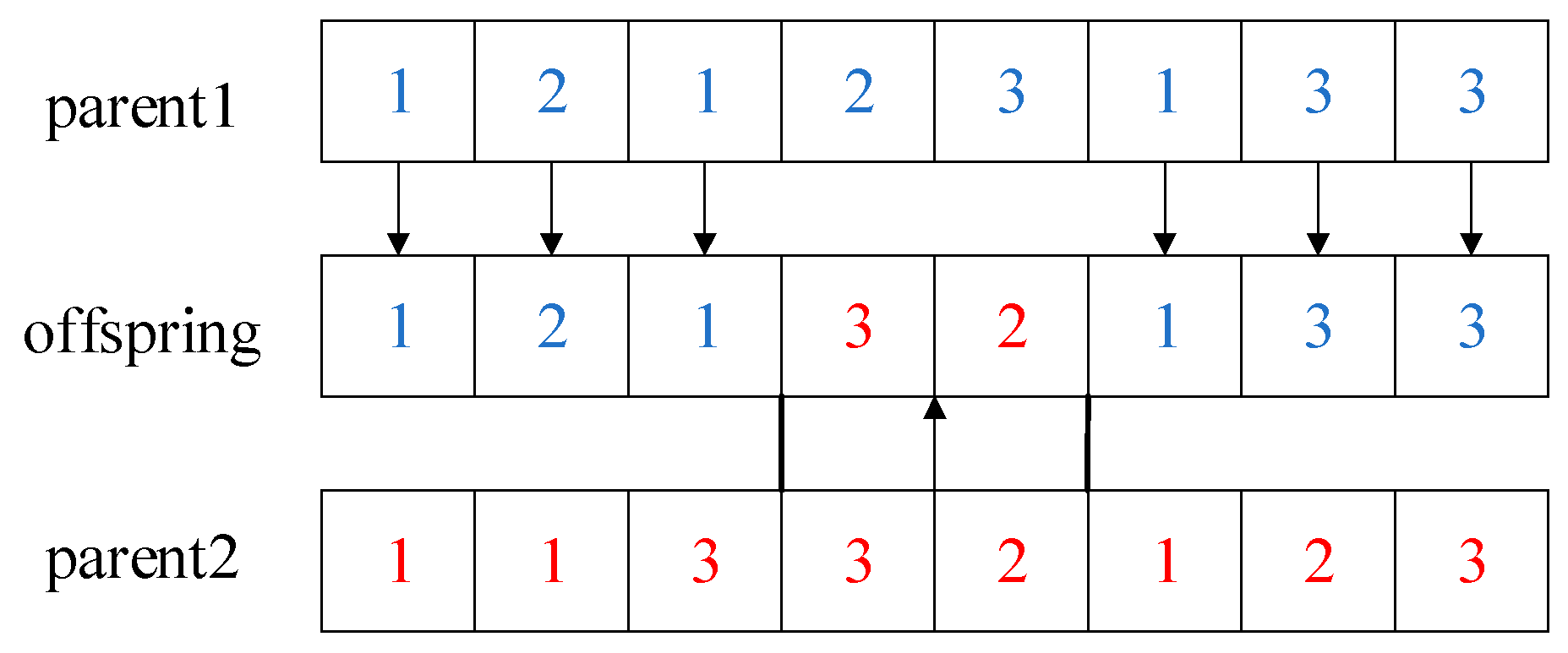
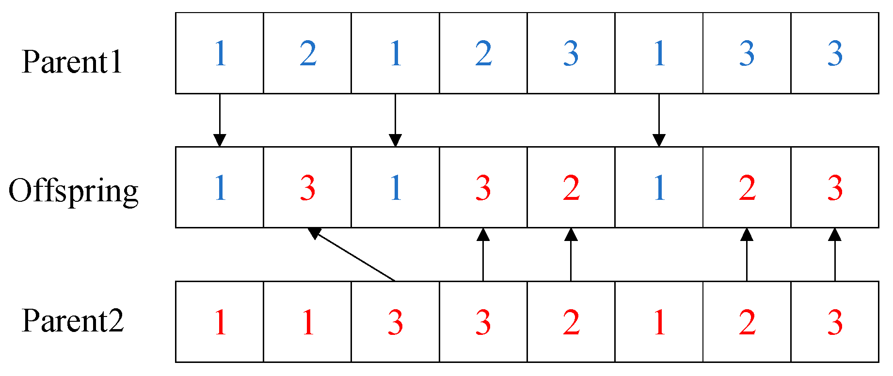
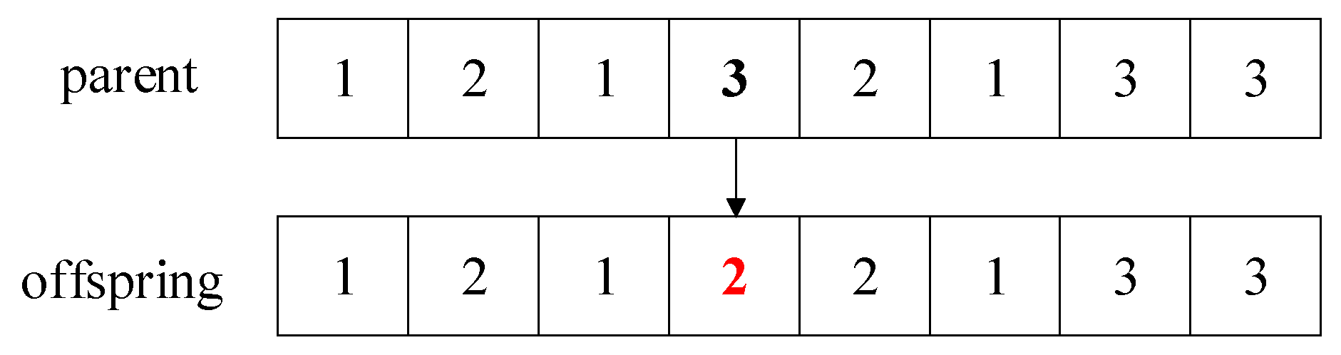
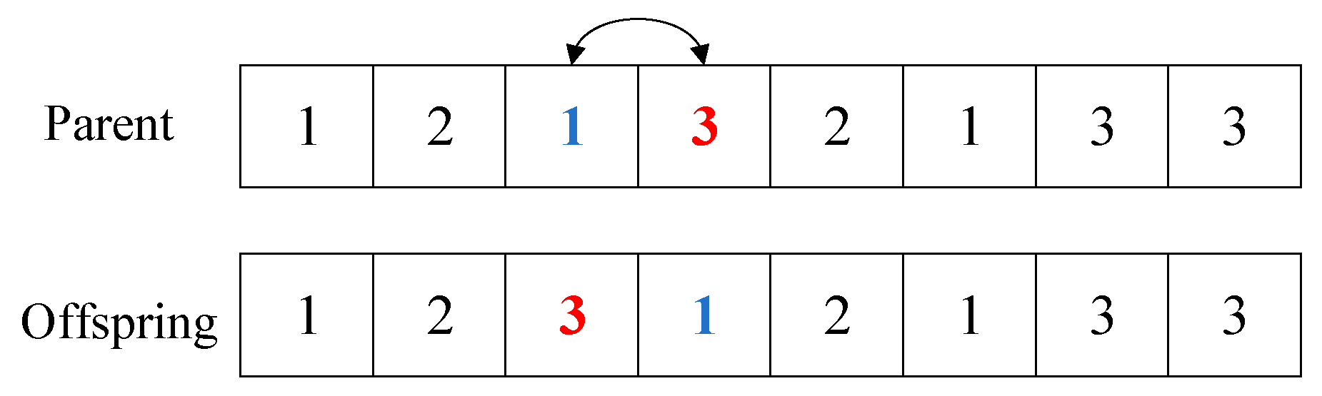
3.1. Description of the Problem

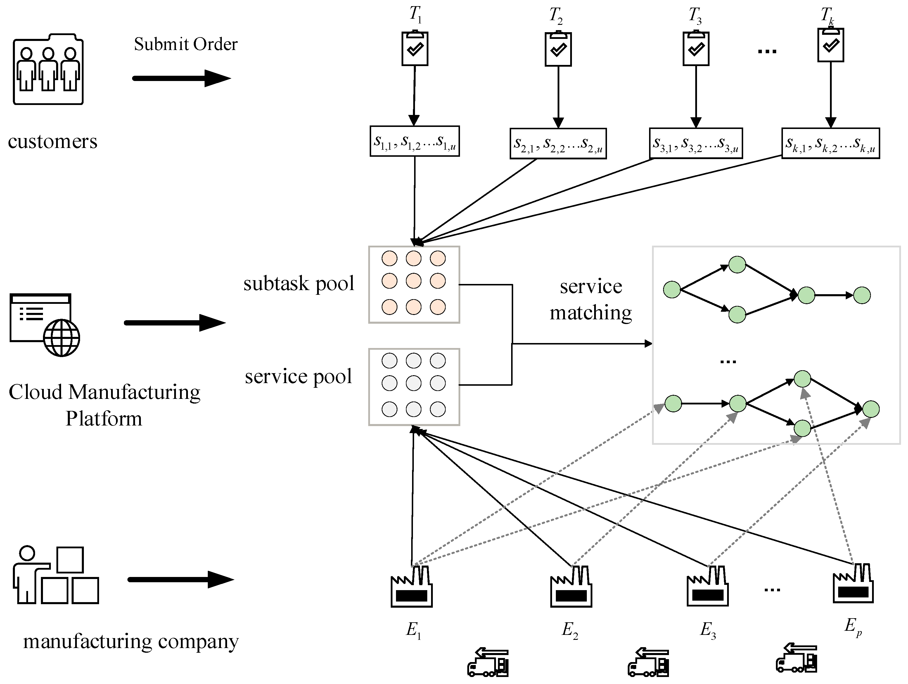
The diagram of the cloud manufacturing model is shown in Figure 1; users continuously provide manufacturing task requirements to the cloud manufacturing platform through the Internet, and manufacturing service providers submit manufacturing services and capabilities to the cloud manufacturing platform system. The cloud manufacturing platform virtualises and services manufacturing resources, generates a set of optimal service scheduling solutions based on user task requirements, and finally sends them to each enterprise manufacturing workshop to complete the execution of specific tasks.
Suppose that under the current cloud manufacturing platform consists of manufacturing service enterprises, denoted as E = E 1 , E 2 , E 3 E m , which the enterprise E m can provide i types of manufacturing services, which the type of services provided by the enterprise is denoted as M m , r . The time, cost, and quality of processing vary from enterprise to enterprise for the same type of processing. Demand tasks from the cloud manufacturing platform user order decomposition, assuming different customers in the cloud manufacturing platform under the submission of single or multiple orders, the cloud platform to receive the allocation for the task processing.
The cloud platform receives the allocation for I tasks to process, denoted as T = T 1 , T 2 , T 3 , , T I , each task includes single or multiple sub-tasks, which may require one or more types of services, and T i can be decomposed into j sub-tasks, denoted as S i , 1 , S i , 2 , S i , 3   S i , j , where the corresponding attributes of each subtask are different and the attributes of the subtasks are denoted by the symbols R i , j . The decomposed subtasks are performed by manufacturing resource providers in the CMfg system by providing manufacturing services. The following assumptions are made for the model.
(1)
Tasks are all available and have the same priority at the beginning;
(2)
That storage buffers are infinite;
(3)
Manufacturers have unlimited manufacturing resources;
(4)
A service provider can handle different types of subtasks, but can only service one subtask at a time;
(5)
Different service providers process the same type of subtask with different costs and times;
(6)
That the quality of service for completing different types of subtasks is different;
(7)
That all subtasks cannot be interrupted once processing has begun.
The relevant parameters involved in the mathematical model are as shown in Table 2:

3.2. Multi-Task Scheduling Model

In this paper, the objective function of the multi-objective optimisation model is established as follows with the optimisation objectives of minimising the workload on the service supply side and maximising the satisfaction on the service demand side in the cloud manufacturing process:
Minimum workload:
f 1 = m i n W
Maximum demand-side satisfaction:
f 2 = max S A
Based on the perspective of service providers, it aims to avoid the overloading of some service providers or idling of some service providers, thus improving the resource utilisation. Load balancing is controlled by calculating the sum of the absolute value of the difference between the working time and the average working time of each service provider, thus protecting the interests of the service providers. The calculation method is shown in Equation (3).
W = m = 1 M | i = 1 I j = 1 J P T i , j m α i , j m 1 M m = 1 M i = 1 I j = 1 J P T i , j m α i , j m |
Cloud manufacturing is the embodiment of the manufacturing-as-a-service concept, and customer satisfaction reflects the degree of customer satisfaction with the resource scheduling service provided by the cloud manufacturing platform, which is one of the key factors in evaluating the success of the cloud manufacturing model. In this paper, we investigate the comprehensive impact of the three dimensions of time, cost, and service quality on customer satisfaction SA.
Customer satisfaction with the total completion cost is expressed as the ratio of the actual completion cost to the maximum acceptable cost to the customer. Since the number of subtasks varies from task to task, for a more accurate representation of satisfaction, a weighted summation is used, with the size of the weight depending on the number of subtasks. When the value is smaller, it represents the lower actual total completion cost required, i.e., the higher the cost satisfaction of the customer. The formula is shown in Equation (4).
R C ¯ = i = 1 I ( ( m = 1 M j = 1 J ( C C i , j + L C i , j , i , j 1 ) / C c o n t , i ) J T i i = 1 I J T i )
where the total cost consists of the manufacturing cost CC and the transport cost LC; the manufacturing cost CC consists of the installation cost SC and the processing cost PC, which are calculated in Equations (5) and (6).
C C i , j = S C i , j m + P C i , j m α i , j m
L C i , j , i , j 1 = T C d m , n α i , j m α i , j 1 n
Customer satisfaction with the total completion time is expressed as the ratio of the actual total cost of completion to the customer’s maximum acceptable cost. The smaller the value, the shorter the actual total completion time required, i.e., the higher the customer’s time satisfaction. Total completion time includes the manufacturing time and logistics time. The calculation is shown in Equation (7).
R T ¯ = i = 1 I ( ( m = 1 M i = 1 I j = 1 J α i , j m C T i , j m / T c o n t , i ) J T i i = 1 I J T i )
In this paper, transport time TT, installation time ST, and processing time PT are considered, and the time required for different sub-tasks and selected service combinations is different. The specific calculations are shown in Equations (8)–(13).
P S T i , j m = S T i , j m                           No   pilot   mission S T i , j 1 m + C T i , j 1 + L T i , j , i , j 1         otherwise
L T i , j , i , j 1 = T T d m , n α i , j m α i , j 1 n
where P S T i , j m represents the predicted start time of sub-task S T i , j when it is processed by service provider m, and L T i , j , ( i , j 1 ) is the time required to transport sub-task S T i , j , which is processed by service provider n to service provider m. If service providers m and n are in the same company, then L T i , j , ( i , j 1 ) = 0 .
C T i , j m = A S T i , j m + P T i , j m α i , j m
A S T i , j m = max P S T i , j m ,   A T m
A T m = max m a x ( C T i , j m ) , A A i , j 1 , i , j α i , j m = 1
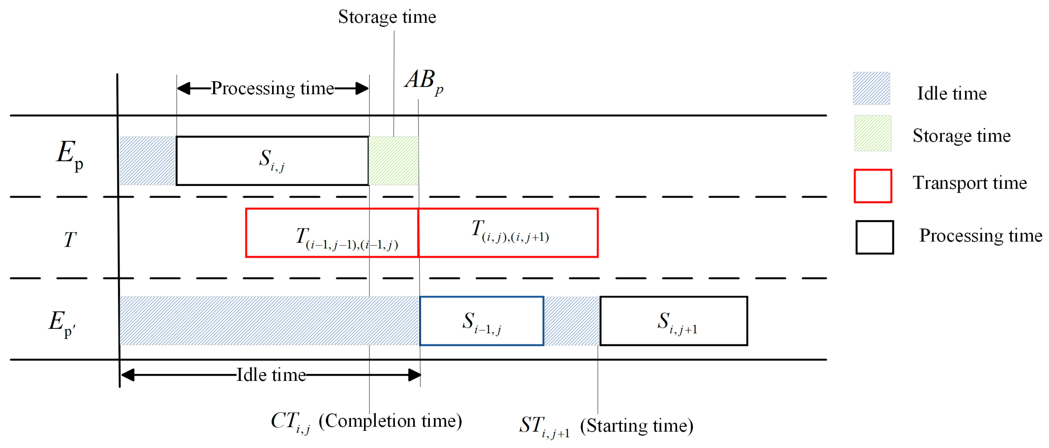
Equation (10) represents the completion time of the subtask at service provider m. The actual start time of the subtask A S T i , j m depends on the actual start time of the task, while the actual start time of the subtask depends on the completion time of the previous subtask C T i , j m and the current service provider’s available time A T m , the earliest time at which the service M can handle the current request for the subtask.
Since each manufacturing service provider in cloud manufacturing is geographically dispersed, the transport time required by the vehicles is non-negligible, so we consider two cases of the number of vehicles, which are finite and infinite. And if the manufacturing service provider completes the sub-tasks if they cannot be transported immediately, they are put into the warehouse for storage. When sub-task S i , j is processed at manufacturing service provider E m , whether its subsequent sub-task S i , j + 1 can start immediately depends on the processing progress of another manufacturing service provider E n , on the one hand, and on the transport time of sub-task S i , j . And when the available time of the vehicle under the manufacturing service provider E m is less than the completion time of the subtask, the subtask is put into the storage area until a free vehicle is available. As shown in Figure 2.
Consequently, a priority transport strategy is considered to minimise transport time. This strategy includes the following: (1) transporting subtasks with services assigned by subsequent subtasks first if immediate initiation is not possible; (2) prioritising subtasks for transportation based on their completion time when either both sub-tasks can start immediately or neither can; (3) otherwise, placing them in the storage area to await transport.
A A i , j = C T i , j 1 + L T i , j , i , j 1     Infinitely A A i , j = max A B p , C T i , j 1 + L T i , j , i , j 1   Limited
Customer satisfaction with total service quality is expressed as the ratio of the actual total quality of completion to the minimum acceptable service to the customer. A higher value means a higher level of satisfaction. The formula is shown in (14).
R S ¯ = i = 1 I m = 1 M j = 1 J α i , j m Q i , j m Q i , j m J T i i = 1 I J T i
By assigning appropriate weights to different factors affecting customer satisfaction, a composite value of SA is calculated to better represent customer satisfaction. The calculation is shown in Equation (15).
S A = m i n w 1 R C ¯ + w 2 R T ¯ + w 3 R S ¯
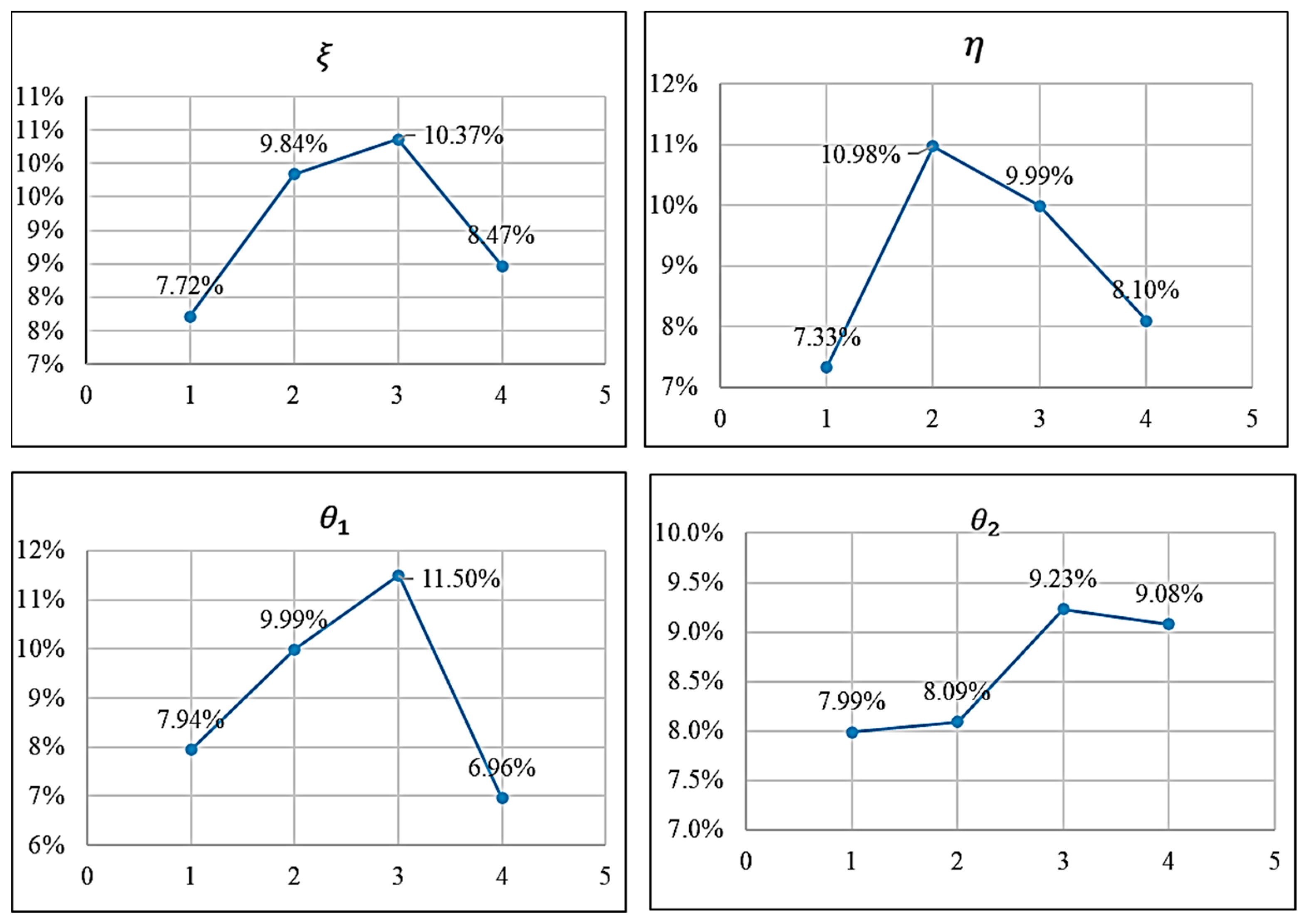
In order to better determine the share of the cost, time, and service quality in customer satisfaction, hierarchical analysis is used. Hierarchical analysis allows for the layering of problems. Depending on the nature of the problem and the objectives to be achieved, the problem is broken down into different components. The interactions and connections between the factors will form an ordered hierarchical model. The relative importance of the hierarchical factors in the model is then expressed quantitatively based on one’s judgement of the objective reality. A comparative judgement matrix was constructed, and the weights for ranking the relative importance of each factor at each level were mathematically determined. Finally, the weights of the relative importance of each factor were comprehensively calculated as the basis for evaluation and selection.
The values of w 1 , w 2 , and w 3 were obtained through the calculation as 0.63, 0.26, and 0.11, and since the evaluation index of service quality is the bigger the better, the value of w 3 is negative for the purpose of unifying the indexes, and the values of w 3 in the final mathematical model are 0.63, 0.26, and −0.11.

3.3. Constraints

(1) The total cost of completion of the assignment cannot be higher than the maximum acceptable cost to the customer.
m = 1 M i = 1 I j = 1 J C C i , j m α i , j m + L C i , j , i , j 1 α i , j m α i , j 1 n C c o n t , i
(2) The total sub-task completion time under each task cannot exceed the latest customer acceptance time.
max C T i , j m + m = 1 M i = 1 I j = 1 J L C i , j , i , j 1 α i , j m α i , j 1 n T c o n t , i
(3) A sub-task can be served by only one enterprise.
m = 1 M α i , j m = 1
(4) The total cost of quality of the assignment cannot be lower than the maximum acceptable quality to the customer.
m = 1 M i = 1 I j = 1 J Q i , j m α i , j m J T i Q c o n t , i
(5) The service attributes that the manufacturing service provider can provide are matched one-to-one with the sub-task attributes in the customer’s order.
R i , j = M m , r   i , j , m ϵ   ( α i , j m = 1 )

4. Improved Three-Stage Genetic Algorithm Design Based on Clustering Algorithm

The model developed in this paper is designed to ensure workload balance while maximising customer satisfaction, so an improved three-stage genetic algorithm is proposed to solve the model. The framework of this research method consists of the Improve 3-Stage Genetic Algorithm (ISGA), which improves the operational efficiency by gradually reducing the search space.
In the first stage, only service allocation and cost constraints are considered. The initial population p is randomly generated based on the attribute consistency principle, and based on the k-means algorithm, the individuals are selected at different clustering centres, and then, the service vectors of each individual are cross-mutated to update the Pareto non-dominated solution set, as well as the non-dominated solution set, according to the Pareto method.
Before starting the second stage, the RTSS heuristic is used to initialise the subtask ordering vectors based on the final population obtained in the first stage, aiming to minimise the idle time based on the progress time of the services and the slack of the subtasks. When iteration η* is the maximum number of iteration times, the success rate of the population is lower than ζ in consecutive iterations, or when the number of iterations reaches θ 1 *, the maximum number of iterations, the first stage is ended and the second stage is started. If both the parent and their descendants either satisfy or do not satisfy the time constraints, then the optimal solution is retained; otherwise, solutions that satisfy the time constraints are retained.
When iterating a maximum of η* maximum iterations, the population’s success rate remains consistently below ζ in consecutive iterations, or when the number of iterations reaches θ 1 + θ 2 * maximum iterations, the third stage begins. The parameters ζ, η, θ 1 , and θ 2 are constant values between 0 and 1, with their specific values detailed in Section 5. Furthermore, in both the first and third stages, a Pareto adaptive method is employed to maintain population diversity and enhance the convergence speed by adjusting the population size based on the performance of descendants. The flow of the improved three-stage genetic algorithm is shown in Figure 3.

4.1. Adaptive Population Size

Pareto introduced the concept of non-dominated solutions for multi-objective problems in 1986. It is defined as follows: suppose for all objectives, f 1 is superior to f 2 ; in that case, we say that f 1 dominates f 2 . If f 1 is not dominated by any other solution, then it is referred to as a non-dominated solution (also known as a non-dominated Pareto optimal solution). Achieving at least one better objective without making any other objective worse is known as Pareto improvement. The Pareto optimal state represents a condition where it is not possible to have more Pareto improvements. Cui et al. [28] proposed the Adaptive Method for Population Size (AMPS) and designed an external archive to store inferior individuals, and the individuals in the external archive still have a chance to enter the next generation. In this paper, we propose a Pareto adaptive population size method; the population size is adjusted according to the dynamic retention of individuals in the current population, which involves the following parameters: minimum population size S N m i n , maximum population size S N m a x , and the current population size SN. The population P consists of a Pareto non-dominated set M and a Pareto dominated set G. The set of Pareto non-dominated solutions includes all Pareto solutions and is continuously updated with each iteration.
In order to maintain the diversity and quality of the population, individuals that are dominant in their parents or offspring will be retained into the next generation. If the parents and offspring do not mutually dominate, the retention rule will change based on the population’s success rate, calculated as SR = SSSN, where SS represents the number of successful searches by individuals in the current population. Generally, if the offspring dominate their parents, the search for offspring is considered successful. If the population’s success rate is high, the population contracts. The success rate of an individual is calculated using the formula
S R i = S C i i t e r i
where S C i is the number of successful searches for individual X i , and i t e r i is the number of iterations for X i . If an individual X i has a low success rate, X i belonging to set G and its descendants X i are often not retained for the next generation; otherwise, X i will be retained. Conversely, if the population’s success rate is low, the population tends to expand. Non-dominated offspring are retained for the next generation. Of course, all population contraction or expansion is based on not exceeding the population size limit. The specific pseudocode is shown in Appendix A.

4.2. Genetic Algorithm

4.2.1. Modes of Coding

For the scheduling optimisation problem, service allocation and subtask sequencing are involved simultaneously. The service allocation problem is to select the appropriate manufacturing service for each subtask, and subtask sequencing is to confirm the processing order of the subtasks from the manufacturing service provider. Therefore, a two-tier coding approach is used. If there are M users, each with I tasks and each with J subtasks, the calculation of the sum of subtasks S can be performed according to Equation (22).
S = m = 1 M i = 1 I j = 1 J s t m n j
The chromosome is encoded in an integer, and the length of the chromosome string is 2 × S. The first part indicates the service assignment, and the change service can process the corresponding subtasks. The second part indicates the processing order of all subtasks. For example, in MS = (2 3 1 2 1 1 3 3 1), the first ‘2’ indicates that the first subtask of task 1 is assigned to the second manufacturing service provider for processing. The second layer is the subtask ordering, where each element represents a subtask of the corresponding task, and the nth occurrence of the same number indicates the nth subtask in the sequence of tasks. For example, for sequences = (1 1 2 1 3 3 2 3), the first ‘1’ represents the first subtask of the first task. The second ‘1’ represents the second subtask of the first task, and the length of the encoding is determined by the number of subtasks. The length of the encoding is determined by the subtask’s. The encoding is 2312133111213323, The service sequence is T 1,1 , M S 2 , T 1,2 , M S 3 , T 2,1 , M S 2 , T 1,3 , M S 1 , T 3,1 , M S 3 , T 3,2 , M S 3 , T 2,2 , M S 1 , T 3,3 , M S 1 which represents the scheduling scheme as shown in Figure 4.

4.2.2. Binary Tournament Selection Method Based on k-Meas Algorithm

Binary tournaments usually randomly select two competitors in the population, and the winner goes to the next generation. However, since there is a probability of selecting similar individuals during the selection process, the k-mean algorithm is combined to improve the diversity of the population. To facilitate the calculation, the objective function value of each individual is standardised, k individuals are randomly selected as the clustering centre, divided into different clusters according to the Euclidean distance between each individual and the cluster, and the clustering centre is constantly updated according to the squared error until it reaches the satisfaction condition. Then, two clusters are randomly selected, and an individual with a minimum Pareto rank and larger crowding distance is selected from any two individuals in each cluster for the next step. The flow of the algorithm is as follows in Appendix B.

4.2.3. Cross-Variation

For service allocation sequences, a two-point crossover operator is used. Two different parents from the current population are selected as the basis for crossover, two crossover points are randomly selected on the chromosomes of the parents, and the segment between the crossover points is copied from one parent to the offspring individual, and the segment outside the crossover points from the other parent is copied to the offspring individual, as shown in Figure 5. Blue numbers indicate genes from parent 1 and red numbers indicate genes from parent 2 in Figure 5.
For subtask ordering sequences, order-based priority-preserving crossover is used. Two different parent individuals from the current population were selected as the basis for crossover, and one or more crossover points were randomly selected in the aligned sequence of parent individuals. The gene segments between the crossover points were copied from one parent individual to the corresponding positions in the offspring, and the remaining blank positions were sequentially complemented by the remaining elements of the other parent individual, as shown in Figure 6. Blue numbers indicate genes from parent 1 and red numbers indicate genes from parent 2 in Figure 6.
For the service assignment sequence, a single point of mutation is used, where an individual from the current population is randomly selected as the subject of the mutation operation to be performed. A randomly selected mutation point in the chromosome of the selected individual, i.e., the location of the gene for which the mutation is to be performed, is re-scheduled to another service based on the mutation rate MR to produce a new offspring. If any infeasible offspring is generated, the available service closest to the currently unavailable service will be reselected and assigned to the corresponding subtask, as shown in Figure 7. Bolded text represents mutated genes and red text represents mutated genes in Figure 7.
For the subtask sequencing sequence, the mutation process will be carried out on the basis of the crossover operator by using the two-point mutation, where an individual is randomly selected from the current population as the object to carry out the mutation operation. Two mutation points, i.e., the gene positions where the mutation is to be performed, will be randomly selected in the chromosome of the selected individual and the two mutation points will be exchanged. The above mutation method avoids the generation of infeasible offspring, as shown in Figure 8. The blue and red numbers in Figure 8 represent the two different mutant genes that were selected.

4.3. Real-Time Task Sequence Scheduling

The purpose of real-time task sequence scheduling is to obtain an initial sub-task sequence based on the first-stage service allocation schedule. This sequence ensures that once the current sub-task processing order is determined, the subsequent sub-tasks become immediately available. During the scheduling process, newly available sub-tasks are sorted based on their slackness, and the sub-task sequencing sequence is updated until all sub-tasks are completed. If the selected sub-tasks have the same slackness, they are sorted randomly. The slackness of sub-tasks represents their urgency, and the calculation method is outlined in Formula (23):
L i , j = T T i , j r t i
where r t i is the total time required to complete the remaining subtasks of the current task according to the given service assignment. To avoid time constraints that cannot be satisfied, all selected subtasks are sorted in ascending order based on their slackness values. Subtasks with the smallest slack value are scheduled first, and subtasks with the same slack value are randomly ordered. The pseudo-code is shown in Appendix C.

5. Case Study

5.1. Description of the Problem

In order to obtain effective parameter combinations and evaluate the performance of the T-SGA, a series of computational experiments was carried out based on four instances. The computer configuration used for these experiments was 8 GB RAM and an Intel(R) Core(TM) i7 CPU @ 1.80 GHz.
In order to test the efficiency of ISGA in multi-objective optimisation solving, six test instances were generated based on different numbers of tasks, sub-tasks, and manufacturing services, shown in Table 3. The ranges of different parameters in the test instances were collected from the company based on the stochastic nature of task execution in the CMfg system. The processing unit time and cost ranged from 10 min to 30 min and $10 to $40, and based on real applications, the unit time and cost were set to range from 10 min to 30 min and $10 to $30. Therefore, considering the confidentiality reasons, the values of these parameters were randomly generated from the scope of the survey. The distance between manufacturing service providers is taken between 100 and 400 km. The average unit logistics cost lc is 5 The average unit logistics time LT is 0.004 days/km.

5.2. Algorithm Parameters and Performance Metrics

5.2.1. Setting Parameters

To obtain a higher-quality solution set with ISGA, it is necessary to determine the values of parameters, such as the population size, ζ, η, θ 1 , and θ 2 . Considering four factor levels and four parameters, a Taguchi orthogonal experiment was employed to determine the optimal parameter combinations. An orthogonal array L 16 (44) was used, and the experiments were conducted using the medium-sized case #03 for comparison. In order to better judge the merits of the parameters, Wang et al. [29] proposed the average response variable (ARV). In each repeated experiment, multiple Pareto nondominated sets were obtained based on different parameter combinations, all Pareto solutions were combined, and Pareto solutions were selected from them to form a new Pareto nondominated set M*. The ratio of the number of solutions belonging to the new nondominated solution set M* under different parameter combinations is calculated; the larger the value, the better the parameter combination. In order to determine the effective initial population size, the ISGA is run independently 20 times on the basis of other parameters with constant values, for which the variation rate is 0.2, the maximum number of iterations is 500, and the difference in each population size is 50. And based on the suggestion of Han et al. [30], the clustering number K is set to 10 to run the ISGA independently 20 times. The ARVs for different parameter combinations are shown in Table 4.
According to the data in the table, the following changes in the ARV for different values of the four parameters are derived, and to better see the changes in the data, the data are represented in Figure 9.

5.2.2. Pareto Front

This paper establishes a multi-objective optimisation model of minimising workload and minimising energy consumption, due to these two optimisation objectives belong to the non-linear relationship, so this paper adopts the method of solving the Pareto-optimal solution set for its calculation, and the image of the Pareto-optimal solution set plotted on the axes of the objective function is the Pareto frontier. In order to better verify the effectiveness of the SGA algorithm, it is compared with the Hybrid Artificial Bee Colony Algorithm (TABC) [31], Modified Genetic Algorithm (MGA) [19], Pareto-based Grouping Discrete Harmony Search algorithm (PGDH) [32], and Multi-objective Particle Warm Optimisation algorithm (MOPSO) [33]
The results of the six random instances are shown in Table 5. From the data in the table, it can be seen that among the solution results of the five algorithms under different algorithms, ISGA takes the best value. Additionally, Figure 10 illustrates that the Pareto frontiers achieved by the ISGA algorithm are superior in comparison to those obtained by the other algorithms. That is, the Pareto solutions obtained by the other four algorithms are almost dominated by the solution set obtained by ISGA.

5.2.3. Evaluation Indicators

In order to verify the effectiveness of the improved algorithm proposed in this paper, the distance with the Lower Bound (DLB), the proximity of the Pareto bound to the Lower Bound, for which the smaller value represents the better solution set, is introduced, adapted from Mansouri et al. [34], and the calculation method is shown in Equations (24) and (25):
D L B W = W i W m i n W m i n Ω
D L B S A = S A i S A m a x S A m a x Ω
Here, Ω denotes the set of all Pareto solutions obtained by the algorithms after 20 runs, and W m i n and S A m a x denote the minimum workload and maximum satisfaction, i.e., the lower bounds of the model solutions obtained by the five algorithms, respectively. W i and S A i denote the ith solution in the algorithms’ Pareto frontiers, where i belongs to Ω. For different problem sizes, the smaller the value of the DLB, the better the set of Pareto solutions obtained by the ISGA. Under different problem sizes, the smaller the value of DLB, the better the set of Pareto solutions it obtains, so it is obvious that ISGA always outperforms the other four algorithms in solving the model, as shown in Table 6.
Due to the non-compliance of the data distribution with the assumptions of a standard t-test, a Robust t-test, also known as the Wilcoxon Signed-Rank Test, was employed. It assesses the differences between our proposed algorithm and the other four algorithms in terms of experimental results. If a p-value is less than 0.05, the differences are considered significant. Table 7 presents the results of the Robust t-test, displaying the corresponding p-values. For most instances, the p-values are below 0.05, indicating significant differences between the ISGA and the other four algorithms. Thus, the effectiveness of the ISGA is further confirmed.
To further assess the efficacy of the ISGA algorithm, this section additionally employs the Inverted Generational Distance (IGD) metric. This metric considers not only the proximity of the generated solutions to the true Pareto front but also the uniformity in the distribution of these solutions. According to the data presented in Table 8, the ISGA significantly outperforms other algorithms in terms of IGD metrics.

5.3. Results Analysis and Discussion

In this subsection, we examine the Pareto solution for the ISGA in ten order tasks. Detailed manufacturing resource information is shown in Table 9 and Table 10. The processing and manufacturing sequences corresponding to partial orders, and the required manufacturing services are shown in Figure 11.
Different automotive parts require different processing services for combined manufacturing. According to the execution process of the cloud platform, after receiving the order information, the cloud platform will pre-process the order, decompose each manufacturing task into multiple sub-tasks with different granularities, and determine its candidate service set. Table 11 shows the processing information after decomposition.
Figure 12 shows the Pareto frontier for cloud manufacturing scheduling optimisation for both the supply and demand sides.
The solution closest to the origin in the Pareto frontier is taken, and its corresponding subtask processing order and the corresponding processing and manufacturing service scheduling scheme are shown in Figure 13. Based on the Pareto solution set, it can be concluded that the range of workloads is between 7.2 and 99.2 min and customer satisfaction is between 0.59 and 0.66. From the manufacturing service provider’s point of view, at the expense of customer satisfaction, the manufacturer can achieve a minimum workload of 7.2 min, which is a 92% reduction in the minimum workload and a significant improvement in resource utilisation. At the same time, every solution in the set of Pareto solutions is satisfying the customer. That is to say, the manufacturing service provider can choose the scheduling solution according to the amount of free resources under the condition of satisfying the demand side of manufacturing services.
Similarly, to better illustrate the necessity of scheduling optimisation research for both supply and demand sides, the ISGA is used for solving the problem, and the optimisation objectives are set to o total completion time, total cost, and total quality, while using the case data. The results of 20 scheduling optimisation solutions are summarised, from which the optimal solution is taken out and a Gantt chart is drawn based on the obtained scheduling. As shown in Figure 14, the blank space between processes indicates that the manufacturer’s processing machine is in an idle state, and comparing the two Gantt charts, it can be seen that the workload is more balanced under the resource scheduling optimisation model oriented towards the supply and demand sides; the resource utilisation rate under the two scenarios is shown in Table 12, and when load balancing is taken into account, the lowest resource utilisation rate of the manufacturing service provider is 71.20%, the highest reaches 93.94%, and the average resource utilisation rate is 76%, while the highest resource utilisation rate of the manufacturer is only 72.56% when load balancing is not considered, and the resource utilisation rate of some manufacturers is less than half, with an average resource utilisation rate of 62.83%. This shows that resource utilisation can be improved when load balancing is considered.

6. Conclusions and Outlook

The research objective of this paper is to solve the optimisation of resource scheduling to satisfy both the supply and demand sides of the service in a cloud manufacturing environment and then to achieve better resource utilisation. Firstly, the demand and supply sides are considered, and the optimisation objectives of minimising load balancing and maximising customer satisfaction are taken as the optimisation objectives, so that the scheduling scheme can meet the demands of both supply and demand sides. Secondly, an improved genetic algorithm is designed, which adopts a staged solution method, while the k-means algorithm is integrated into the selection operator to improve the diversity of the population; a real-time sequential scheduling strategy is adopted, which improves the quality of the understanding. Finally, by comparing and analysing with the other four heuristic algorithms, the effectiveness and efficiency of the ISGA in solving the supply-demand dual-issue coordinated scheduling problem is verified.
This paper lays theoretical foundations and provides empirical insights for multi-objective multi-task scheduling optimisation in cloud manufacturing environments. Nevertheless, given the diversity of cloud manufacturing scenarios, substantial research opportunities remain. Future efforts should encompass a broader array of scheduling objectives, including carbon emissions, water usage, labour costs, and order batching, to address the cloud manufacturing multi-task scheduling challenge more holistically. Additionally, incorporating dynamic factors, such as machine breakdowns, rush orders, and schedule changes, into the scheduling process is crucial, enabling rapid task reassignment and flexible priority adjustments to accommodate evolving production demands.

Author Contributions

Conceptualisation, Q.Z.; Methodology, J.D.; Resources, Y.Z.; Writing—original draft, N.L.; Writing—review and editing, J.Q. All authors have read and agreed to the published version of the manuscript.

Funding

This research received no external funding.

Data Availability Statement

The data are contained within the article, and the corresponding author can be contacted if there are other requests.

Conflicts of Interest

The authors declare no conflicts of interest.

Appendix A. Pseudo-Code for Adaptive Population Size Algorithm

Algorithm A1: Pareto-based adaptive population size method
For i = 1: SN
    If  X i dominated by X i
        Reserve X i into the next generation
    If  X i is dominated by X i
        Reserve X i into the next generation
Else
  Calculate success rate SR of all individuals
  If SR > rand // shrink the population
    Calculate success rate s r i of the ith individual
      If  X i ϵ G && s r i < rand && SN>  S N m i n
        SN = SN − 1
      End if
  Else // expand the population
      If SN < S N m a x
          Reserve X i into the next generation and SN = SN + 1
      End if
End for
    Update M and G

Appendix B. Clustering Algorithm Kmeans Pseudo-Code

Algorithm A2: Procedure of k-means cluster in selection operator
Begin
  Normalised the objective function of each individual p
   Choose   Kindividuals   randomly   as   the   centre   of   clusters ,   set   i t e r = 1 ,   E 0 = 0
  While  i t e r C m a x i t e r
      Calculate the Euclidean distance between the individuals and K centres
      Assign each individual to a cluster based on the smallest Euclidean distance.
  •       Calculate   the   sum   of   the   squared   errors   E i t e r = p = 1 s o p k = 1 K z p k f p ¯ μ k 2 ,
  •       Where   μ k   denotes   objective   function   vector   of   the   k th   cluster   centre   and   sop = size   of   population .   z p k = 1 ,   if   individual   p   in   the   cluster   C k ,   else   z p k = 0 .
  If  i t e r > 1
        If  E i t e r = E i t e r 1
          break.
        Else
           Update   its   centre   μ k .
        Endif
  Endif
   i t e r = t e r + 1 16.
  Endwhile
End

Appendix C. Real-Time Task Sequence Scheduling Pseudo-Code

Algorithm A3: Real-Time sequence scheduling
While  h u = 1 U K u // h is the total number of sequenced subtasks
    If the subtasks are newly available at the current time
        Select the newly available subtasks
        Calculate the laxity of the selected subtasks
        Sequence the selected subtasks according to the laxity value
        If two or more selected subtasks have the same laxity value
            Sequence the selected subtasks that have the same laxity value randomly
        End if
        Add the sequence record to the subtask sequence vector
       h = h + δ // δ is the number of selected subtasks at each time
End while

References

  1. Rashidifar, R.; Bouzary, H.; Chen, F.F. Resource Scheduling in Cloud-Based Manufacturing System: A Comprehensive Survey. Int. J. Adv. Manuf. Technol. 2022, 122, 4201–4219. [Google Scholar] [CrossRef]
  2. Bouzary, H.; Chen, F.F.; Krishnaiyer, K. Service Matching and Selection in Cloud Manufacturing: A State-of-the-Art Review. Procedia Manuf. 2018, 26, 1128–1136. [Google Scholar] [CrossRef]
  3. Liu, B.; Zhang, Z. QoS-Aware Service Composition for Cloud Manufacturing Based on the Optimal Construction of Synergistic Elementary Service Groups. Int. J. Adv. Manuf. Technol. 2017, 88, 2757–2771. [Google Scholar] [CrossRef]
  4. Goodarzi, E.V.; Houshmand, M.; Valilai, O.F.; Ghezavati, V.; Bamdad, S. Manufacturing Cloud Service Composition Based on the Non-Cooperative and Cooperative Game Theory. In Proceedings of the 2020 IEEE International Conference on Industrial Engineering and Engineering Management (IEEM), Singapore, 14–17 December 2020; pp. 1122–1125. [Google Scholar]
  5. Qian, C.; Zhang, Y.; Liu, Y.; Wang, Z. A Cloud Service Platform Integrating Additive and Subtractive Manufacturing with High Resource Efficiency. J. Clean. Prod. 2019, 241, 118379. [Google Scholar] [CrossRef]
  6. Valizadeh, S.; Fatahi Valilai, O.; Houshmand, M. Flexible Flow Line Scheduling Considering Machine Eligibility in a Digital Dental Laboratory. Int. J. Prod. Res. 2020, 58, 6513–6531. [Google Scholar] [CrossRef]
  7. Jian, C.F.; Wang, Y. Batch Task Scheduling-Oriented Optimization Modelling and Simulation in Cloud Manufacturing. Int. J. Simul. Model. 2014, 13, 93–101. [Google Scholar] [CrossRef]
  8. Yang, D.; Liu, Q.; Li, J.; Jia, Y. Multi-Objective Optimization of Service Selection and Scheduling in Cloud Manufacturing Considering Environmental Sustainability. Sustainability 2020, 12, 7733. [Google Scholar] [CrossRef]
  9. Zeynivand, M.; Ranjbar, H.; Radmanesh, S.-A.; Fatahi Valilai, O. Alternative Process Routing and Consolidated Production-Distribution Planning with a Destination Oriented Strategy in Cloud Manufacturing. Int. J. Comput. Integr. Manuf. 2021, 34, 1162–1176. [Google Scholar] [CrossRef]
  10. Hu, Y.; Zhu, F.; Zhang, L.; Lui, Y.; Wang, Z. Scheduling of Manufacturers Based on Chaos Optimization Algorithm in Cloud Manufacturing. Robot. Comput.-Integr. Manuf. 2019, 58, 13–20. [Google Scholar] [CrossRef]
  11. Li, W.; Zhu, C.; Yang, L.T.; Shu, L.; Ngai, E.C.-H.; Ma, Y. Subtask Scheduling for Distributed Robots in Cloud Manufacturing. IEEE Syst. J. 2017, 11, 941–950. [Google Scholar] [CrossRef]
  12. Tong, H.; Zhu, J. A Novel Method for Customer-Oriented Scheduling with Available Manufacturing Time Windows in Cloud Manufacturing. Robot. Comput.-Integr. Manuf. 2022, 75, 102303. [Google Scholar] [CrossRef]
  13. Akbaripour, H.; Houshmand, M.; Van Woensel, T.; Mutlu, N. Cloud Manufacturing Service Selection Optimization and Scheduling with Transportation Considerations: Mixed-Integer Programming Models. Int. J. Adv. Manuf. Technol. 2018, 95, 43–70. [Google Scholar] [CrossRef]
  14. Zhou, J.; Yao, X. A Hybrid Approach Combining Modified Artificial Bee Colony and Cuckoo Search Algorithms for Multi-Objective Cloud Manufacturing Service Composition. Int. J. Prod. Res. 2017, 55, 4765–4784. [Google Scholar] [CrossRef]
  15. Delaram, J.; Valilai, O.F. A Mathematical Model for Task Scheduling in Cloud Manufacturing Systems Focusing on Global Logistics—ScienceDirect. Procedia Manuf. 2018, 17, 387–394. [Google Scholar] [CrossRef]
  16. Zhang, W.; Ding, J.; Wang, Y.; Zhang, S.; Xiong, Z. Multi-Perspective Collaborative Scheduling Using Extended Genetic Algorithm with Interval-Valued Intuitionistic Fuzzy Entropy Weight Method. J. Manuf. Syst. 2019, 53, 249–260. [Google Scholar] [CrossRef]
  17. Zheng, H.; Feng, Y.; Tan, J. A Hybrid Energy-Aware Resource Allocation Approach in Cloud Manufacturing Environment. IEEE Access 2017, 5, 12648–12656. [Google Scholar] [CrossRef]
  18. Zhou, L.; Zhang, L.; Fang, Y. Logistics Service Scheduling with Manufacturing Provider Selection in Cloud Manufacturing. Robot. Comput.-Integr. Manuf. 2020, 65, 101914. [Google Scholar] [CrossRef]
  19. Li, F.; Zhang, L.; Liao, T.W.; Liu, Y. Multi-Objective Optimisation of Multi-Task Scheduling in Cloud Manufacturing. Int. J. Prod. Res. 2019, 57, 3847–3863. [Google Scholar] [CrossRef]
  20. Zhou, L.; Zhang, L.; Horn, B.K.P. Collaborative Optimization for Logistics and Processing Services in Cloud Manufacturing. Robot. Comput.-Integr. Manuf. 2021, 68, 102094. [Google Scholar] [CrossRef]
  21. Wu, Q.; Xie, N.; Zheng, S. Integrated Cross-Supplier Order and Logistic Scheduling in Cloud Manufacturing. Int. J. Prod. Res. 2022, 60, 1633–1649. [Google Scholar] [CrossRef]
  22. Helo, P.; Phuong, D.; Hao, Y. Cloud Manufacturing—Scheduling as a Service for Sheet Metal Manufacturing. Comput. Oper. Res. 2019, 110, 208–219. [Google Scholar] [CrossRef]
  23. Ahn, G.; Hur, S. Multiobjective Real-Time Scheduling of Tasks in Cloud Manufacturing with Genetic Algorithm. Math. Probl. Eng. 2021, 2021, 1305849. [Google Scholar] [CrossRef]
  24. Jafarnejad Ghomi, E.; Masoud Rahmani, A.; Nasih Qader, N. Service Load Balancing, Task Scheduling and Transportation Optimisation in Cloud Manufacturing by Applying Queuing System. Enterp. Inf. Syst. 2019, 13, 865–894. [Google Scholar] [CrossRef]
  25. Li, F.; Liao, T.W.; Zhang, L. Two-Level Multi-Task Scheduling in a Cloud Manufacturing Environment. Robot. Comput.-Integr. Manuf. 2019, 56, 127–139. [Google Scholar] [CrossRef]
  26. Yuan, M.; Cai, X.; Zhou, Z.; Sun, C.; Gu, W.; Huang, J. Dynamic Service Resources Scheduling Method in Cloud Manufacturing Environment. Int. J. Prod. Res. 2021, 59, 542–559. [Google Scholar] [CrossRef]
  27. Shi, Y.; Luo, L.; Guang, H. Research on Scheduling of Cloud Manufacturing Resources Based on Bat Algorithm and Cellular Automata. In Proceedings of the 2019 IEEE International Conference on Smart Manufacturing, Industrial & Logistics Engineering (SMILE), Hangzhou, China, 20–21 April 2019; pp. 174–177. [Google Scholar]
  28. Cui, L.; Li, G.; Zhu, Z.; Lin, Q.; Wen, Z.; Lu, N.; Wong, K.-C.; Chen, J. A Novel Artificial Bee Colony Algorithm with an Adaptive Population Size for Numerical Function Optimization. Inf. Sci. 2017, 414, 53–67. [Google Scholar] [CrossRef]
  29. Wang, L.; Wang, S.; Liu, M. A Pareto-Based Estimation of Distribution Algorithm for the Multi-Objective Flexible Job-Shop Scheduling Problem. Int. J. Prod. Res. 2013, 51, 3574–3592. [Google Scholar] [CrossRef]
  30. Han, J.; Kamber, M.; Pei, J. Methods. In Data Mining: Concepts and Techniques; Elsevier: Amsterdam, The Netherlands, 2012; pp. 443–495. ISBN 978-0-12-381479-1. [Google Scholar]
  31. Li, J.; Pan, Q. Solving the Large-Scale Hybrid Flow Shop Scheduling Problem with Limited Buffers by a Hybrid Artificial Bee Colony Algorithm. Inf. Sci. 2015, 316, 487–502. [Google Scholar] [CrossRef]
  32. Gao, K.Z.; Suganthan, P.N.; Pan, Q.K.; Chua, T.J.; Cai, T.X.; Chong, C.S. Pareto-Based Grouping Discrete Harmony Search Algorithm for Multi-Objective Flexible Job Shop Scheduling. Inf. Sci. 2014, 289, 76–90. [Google Scholar] [CrossRef]
  33. Abdullah, M.; Al-Muta’a, E.A.; Al-Sanabani, M. Integrated MOPSO Algorithms for Task Scheduling in Cloud Computing. J. Intell. Fuzzy Syst. 2019, 36, 1823–1836. [Google Scholar] [CrossRef]
  34. Mansouri, S.A.; Aktas, E.; Besikci, U. Green Scheduling of a Two-Machine Flowshop: Trade-off between Makespan and Energy Consumption. Eur. J. Oper. Res. 2016, 248, 772–788. [Google Scholar] [CrossRef]
Figure 1. Cloud manufacturing flowchart.
Systems 12 00133 g001
Figure 2. Scheduling instructions under vehicle restrictions.
Systems 12 00133 g002
Figure 3. Flowchart of the improved three-stage genetic algorithm.
Systems 12 00133 g003
Figure 4. Modes of coding.
Systems 12 00133 g004
Figure 5. Two-point crossover.
Systems 12 00133 g005
Figure 6. Order-based priority-preserving crossover.
Systems 12 00133 g006
Figure 7. Single-point mutation.
Systems 12 00133 g007
Figure 8. Two-point mutation.
Systems 12 00133 g008
Figure 9. ARVs for different values.
Systems 12 00133 g009
Figure 10. Pareto frontiers for different algorithms under different arithmetic cases.
Systems 12 00133 g010
Figure 11. Order processing sequence.
Systems 12 00133 g011
Figure 12. Case Pareto frontier for supply and demand sides.
Systems 12 00133 g012
Figure 13. Supply and demand bilateral scheduling optimisation results Gantt chart.
Systems 12 00133 g013
Figure 14. Gantt chart of optimisation results without considering load balancing scheduling.
Systems 12 00133 g014
Table 1. Summary of research objectives.
Demand SideSupply Side
AuthorYearCostTimeQuality of ServiceCustomer
Satisfaction
Energy
Consumption
Workloads
Li et al. [11]2017
Akbaripour et al. [13]2017
Zhou et al. [14]2017
Delaram et al. [15]2018
Zhang et al. [16]2019
Zheng et al. [17]2019
Qian et al. [5]2019
Zhou et al. [18]2020
Li et al. [19]2020
Zhou et al. [20]2021
Wu et al. [21]2022
Tong et al. [12]2022
Table 2. Related symbols and meanings.
NotationHidden Meaning
T i Task i = 1, 2, 3…I
ITotal number of tasks
J T i Number of subtasks in task i
S T i , j Subtask j of task i,j = 1, 2, 3…J
R i , j Attributes of the jth subtask of task i
E m Manufacturer m = 1, 2, 3…M
M m , r Attributes of services provided by manufacturer E m
P C i , j m Processing cost of sub-task j of task i at manufacturer m
S C i , j m Installation cost of subtask j of task i at manufacturer m
C C i , j m Manufacturing cost of sub-task j of task i at manufacturer m
P T i , j m Processing time of task i’s subtask j at manufacturer m
S T i , j m Subtask j of task i’s installation time at manufacturer m
Q i , j m Quality of sub-task j of task i at manufacturer m
T C Cost per unit distance travelled
T T Time per unit distance travelled
d m , n Distance from manufacturer m to manufacturer n
A S T i , j m Start time of subtask j of task i at manufacturer m
C T i , j m Completion time of sub-task j of task i at manufacturer m
A T m Available time at manufacturer m
P S T i , j m Preset start time of task i’s subtask j at manufacturer m
α i , j m Whether sub-task j of task i is processed at manufacturer m or not
C c o n t , i Maximum acceptable cost for task i
T c o n t , i Latest acceptable time for task i
A B p Earliest available time for vehicle at E p
Q c o n t , i Minimum acceptable product quality for task i
WTotal average workload
R C ¯ Weighted cost satisfaction
R T ¯ Weighted time satisfaction
R S ¯ Weighted quality satisfaction
w i Weights of different attributes in satisfaction
α i , j m 1 if subtask S T i , j is processed by E m ; 0 otherwise
Table 3. Test case information.
CaseTotal Number of TasksRange of Number of SubtasksTotal Number of SubtasksNumber of Manufacturing Services
151–5183
2101–7495
3153–7765
4204–812710
5404–825415
6604–838120
Table 4. ARVs under orthogonal experiments.
Serial Numberξη θ 1 θ 2 ARV
111115.06%
212229.61%
3133312.64%
414443.55%
521238.09%
6221412.04%
723419.61%
824329.61%
9313411.12%
1032439.61%
1133128.09%
12342112.64%
1341425.06%
14423112.64%
1543249.61%
1644136.58%
Table 5. Pareto-optimal solutions for different algorithms.
WorkloadSatisfaction
ISGAMGAMOPSOABCHSISGAMGAMOPSOABCHS
12843.246.841.656.80.6360.6390.6470.6530.724
28.8127.611.226.40.5550.5770.5740.5780.701
35.632.42010600.5260.5920.5620.5820.632
421.291.614041.22400.5880.6420.670.5920.700
5103256.12301374280.6210.7190.7130.6710.765
6545.3703.9549.1628.68410.7240.8680.84730.76310.901
Table 6. DLB of different algorithms in different cases.
WorkloadSatisfaction
ISGAMGAMOPSOABCHSISGAMGAMOPSOABCHS
11.78464.0789.4966.8119.1010.0640.0790.080.0940.205
23.0592.2567.8065.1596.9560.0490.090.110.0830.313
33.72810.7657.43111.88917.2630.0210.1490.0670.0590.213
43.1447.29816.0246.02619.2070.0310.1340.1370.0390.21
51.6253.0843.7692.05226.37290.0170.1980.1460.0900.267
60.99101.89052.05240.81182.93200.09310.2913 0.22980.20900.2830
Table 7. Robust t-test results.
#01#02#03#04#05#06
MGA1.249 × 10−50.00280890.012.558 × 10−50.01992.58 × 10−5
MOPSO0.001220.0012890.0020.011980.01993.25 × 10−5
ABC0.00610.015510.0105.01 × 10−60.00130.0009
HS0.01460.014690.02501.104 × 10−53.14 × 10−81.91 × 10−8
Table 8. IGD values under different algorithms.
IGD#01#02#03#04#05#06
ISGA0.02270.01240.88603.48190.00590.01079
MGA2.62110.01325.15839.93308.39726.90664
MOPSO5.93940.04442.733525.111923.50350.68788
ABC0.02170.04381.23245.25280.58770.0230
HS10.87180.77019.546225.364976.565228.71873
Table 9. Manufacturer and manufacturing resource information.
ManufacturersServiceTime/minProcessing Cost/$Set Cost/$Quality (%)
1turn12291592
drilling33172486
soldered28181995
planning19201694
2bores23232082
soldered17182295
turn35151992
3punch18181789
mill26172395
soldered34172194
4planning12271692
turn26112283
drilling38202594
5bores36232495
planning16182398
soldered20241992
Table 10. Distance between manufacturers.
km12345678910
10355.4245.5272.320.2126.255.210.819.3170.3
2355.40100.221.5153.9200.224.515.4148.9298.1
3245.5100.20292.660.228.773.222.221.118.4
4272.321.5292.60113.5175.8178.1301.6156.9279.3
520.2153.960.2113.5041.616.512118.616
6126.2200.228.7175.841.6019.663.192.4186.2
755.224.573.2178.116.519.6016.648.932.5
810.815.422.2301.612163.116.60102.764.3
919.3148.921.1156.918.692.448.9102.70136.1
10170.3298.118.4279.316186.232.564.3136.10
Table 11. Scheduling task information.
TaskNumber of SubtasksSubtask
14Valve/Crankcase/Connecting rod/Oil pan
23Gear housing/Oil pan/EGR passage
34Connecting rod/Oil pan/Gear housing/EGR passage
46Gear housing/Oil pan/EGR passage/Valve/Crankcase/Clutch housing
54Gear housing/Clutch housing/EGR passage/Valve
67Gear housing/Oil pan/Valve/Crankcase/Clutch housing/Connecting rod
73Crankcase/Connecting rod/Oil pan
86Gear housing/Clutch housing/EGR passage/Valve/Crankcase/Oil pan
95Gear housing/Connecting rod/Valve/Crankcase/Clutch housing
107Crankcase/Clutch housing/EGR passage/Valve/Gear housing/Oil pan
Table 12. Whether to consider load balancing resource utilisation comparison.
Consider Load BalancingDo Not Consider Load Balancing
Task1234512345
Load Time148107144148146155100134142165
Total Boot Time157.5180.4202.2203176.6234.7243.7185.4228227.4
Resource Utilisation93.9%59.3%71.2%72.9%82.6%66.%41.%72.2%62.3%72.5%
Average Utilisation76.00%62.83%
Disclaimer/Publisher’s Note: The statements, opinions and data contained in all publications are solely those of the individual author(s) and contributor(s) and not of MDPI and/or the editor(s). MDPI and/or the editor(s) disclaim responsibility for any injury to people or property resulting from any ideas, methods, instructions or products referred to in the content.

