Abstract
Considering the characteristics of both quality and quantity losses in fresh produce as well as the existence of spot markets, optimal retailer ordering, pricing, and freshness-keeping decisions through the single ordering policy (firm ordering only or option ordering only) and the mixed ordering policy (firm ordering and option ordering simultaneously) are constructed based on option contracts and analyzed for the retailer under different ordering policies. The results show that there is a unique optimal pricing, ordering, and freshness-keeping decision under all three ordering policies, but there is no joint decision. The optimal freshness-keeping and retail price under the mixed ordering policy are lower than those under the option ordering only but higher than those under the firm ordering only. When only a single order can be placed, the retailer’s optimal ordering policy is determined by demand risk. When all three ordering policies are available, the optimal ordering policy for the retailer is the mixed ordering policy. A spot market will weaken the role of option contracts in mitigating supply chain risks, and the larger the risk, the more significant the role of the spot market.
1. Introduction
Fresh produce refers to products that have a short shelf life and are prone to decay due to changes in the environment and external physical factors, such as vegetables, fruits, meats, eggs, seafood, etc. Due to their perishable characteristic, fresh produce faces many issues during transportation, including quality drop and quantity loss, resulting in high circulation loss rates and causing significant damage to retailers and suppliers [1,2,3]. The average rate of circulation losses in the fresh product industry is alarmingly high in China, standing at 25–30%, leading to annual losses of more than RMB 150 billion, which are mainly due to ineffective cold chain preservation measures [4,5]. This rate is more than twice as high as that in developed Western economies [6]. These massive losses in circulation do not satisfy the increasing expectations of customers who are becoming more conscious of the freshness and quality of fresh produce [7,8]. Therefore, reducing the circulation losses of fresh produce and improving their quality and freshness level have become significant challenges for fresh produce supply chains.
Supply chain contracts, such as buyback, revenue sharing, and quantity discount contracts, have been validated by academic researchers as effective methods to mitigate the risk of stochastic demand in supply chains [9,10,11]. In recent years, fresh produce retailers have increasingly adopted option contracts, especially those that combine pure call options with wholesale prices, to hedge risks, such as demand and supply uncertainty, as well as price volatility [4,12]. Option contracts are derivative instruments that give the holder the right, but not the obligation, to buy or sell a particular item at a predetermined price within a specified period. Therefore, call option contracts not only mitigate the risk of uncertain demand from the retailer and ensure supply but also alleviate the production burden on the supplier and the potential for under- or over-production. Option contracts have seen widespread application in industries, including the fashion, IT, semiconductors, and electricity sectors [13]. For example, China Telecom procures products worth more than RMB 100 billion annually from its suppliers through wholesale price and call option contracts [4]. Hewlett-Packard procures over 35% of its components through option contracts [14]. Nike uses option contracts to hedge against expected but unconfirmed future transactions with third-party suppliers [15]. In recent years, an increasing number of agricultural supply chain members have turned to option contracts as a means of hedging against the risks of demand uncertainty and purchase price fluctuations. For instance, in Hainan province, China, several flower operating companies offer flower options for customers around the world [4]. In Ishikawa, Japan, buyers such as traditional fresh stores and restaurants have been ordering vegetables from an agricultural agency established by local farmers through option contracts since 2008 [16].
With option contracts, the retailer must not only trade-off the impacts on their own profit between overage and underage, between excessive freshness-keeping and insufficient freshness-keeping, and between low pricing and high pricing, but also trade-off in relation to the high costs of purchasing against the benefits of increased flexibility. If the retailer orders more through option contracts and less through wholesale price contracts, the underage cost may be low and flexibility may be high, but if market demand is also high, the purchase cost will increase. If the retailer orders more through wholesale price contracts and less through option contracts, the purchase cost will be low, the overage cost may be high, and flexibility may be low. Freshness-keeping efforts present a higher challenge for the retailer when making ordering, pricing, and freshness-keeping decisions with option contracts. The retailer must balance not only the flexibility of option availability and option ordering costs but also the level of freshness-keeping efforts and preservation costs. Therefore, retail price and order quantity, as well as the level of freshness-keeping efforts, need to be decided to maximize the retailer’s profits. The following key issues will be explored:
- (1)
- How do fresh produce retailers make optimal pricing, ordering, and freshness-keeping decisions simultaneously in scenarios with freshness-keeping efforts and option contracts?
- (2)
- How do spot markets influence a fresh produce retailer’s optimal decisions considering option contracts and freshness-keeping efforts?
- (3)
- What are the conditions in which single ordering and mixed ordering are more advantageous for to retailer?
In this paper, we creatively introduce option contracts as a financial derivative and spot markets into fresh produce supply chains while considering freshness-keeping efforts and obtain some novel insights that are different from previous similar studies. First, we obtain optimal ordering, pricing, and freshness-keeping decisions for the retailer with option contracts in a fresh produce supply chain that considers both quality drop and quantity loss. Second, in the above context, we investigate the optimal decisions for the retailer when they use single ordering and mixed ordering policies, respectively, and systematically compare the effects of the different ordering policies on the retailer’s profits. Third, we explore the effects of demand risk, contract parameters, circulation losses, and spot market price on retailer ordering, pricing, freshness-keeping decisions, and maximum expected profits. This study combines financial derivatives with fresh produce supply chains, which provides new application scenarios for the theory and expands the research scope of pricing and newsvendor problems in the context of fresh produce, which will help to improve the efficiency of fresh produce circulation and increase the ability of fresh produce sellers to resist risks, in order to help the stable and efficient development of fresh produce supply chains.
The rest of the paper has been structured in the following manner. Section 2 presents a review of the relevant literature. Section 3 provides a description of the model and a set of assumptions. Section 4 and Section 5 present the optimal ordering, pricing, and freshness-keeping decisions for retailers in the case of single ordering and mixed ordering policies, respectively. Section 6 presents the analysis results of numerical examples and provides related management inspirations. Section 7 discusses and concludes this paper and proposes possible directions for further research.
2. Literature Review
There are three main streams in the literature that are relevant to our study, which include the management of supply chains for deteriorating products, the operational management of supply chains considering freshness-keeping efforts, and the use of option contracts to hedge supply chain risks.
2.1. Management of Supply Chains for Deteriorating Products
The value of fresh produce deteriorates significantly over time at a rate that is highly dependent on temperature and humidity [17]. Therefore, the supply chain management of deteriorating products, especially fresh produce, faces huge challenges. Extensive research has been conducted by many academics on the problem of ordering and pricing deteriorating products. Cai et al. [18] demonstrated the relationship between the optimal selling price and optimal inventory level for deteriorating products. Many scholars have researched the issues relating to the ordering or pricing of perishable goods from different perspectives [19,20,21,22]. The abovementioned scholars only examined the ordering or pricing decisions, while other scholars have investigated joint ordering and pricing decisions. Qin, Wang and Wei [2] and Rabbani et al. [23] considered the pricing and ordering problems related to fresh produce with quality and physical quantity deterioration simultaneously to seek the maximum total system profit. Additionally, the coordination of supply chains for deteriorating products has been investigated by scholars through the application of revenue sharing contracts [24,25,26].
2.2. Operational Management of Freshness-Keeping Efforts
There is a large body of literature on the operational management of fresh produce supply that considers freshness-keeping efforts. Cai, Chen, Xiao and Xu [1] pointed out that fresh products suffer from quantity losses and quality drops (where quality refers to freshness) during transportation and that the freshness of fresh products at the time of arrival in the target market affects market demand. Preservative technologies have recently gained significant attention from researchers due to their potential to preserve the quality of deteriorating goods. Dye and Hsieh [27] aimed to maximize total profit per unit of time by searching for optimal schedules for replenishment and investment strategies in preservation technology. Liu et al. [28] conducted research on how information sharing affects supply chain equilibrium decisions when the supplier is responsible for maintaining the freshness of a product. Some scholars have designed a coordination mechanism for fresh produce supply chains with freshness-keeping efforts. Zheng et al. [29] designed a fresh-keeping cost-sharing contract and a fresh-keeping cost- and revenue-sharing contract to coordinate fresh product supply chains. Mohammadi et al. [30] developed a novel coordination mechanism that not only reduces the perishability of fresh products but also increases the profitability of supply chain members. Some scholars have researched fresh produce supply chains with outsourced logistics and cold-chain service levels [31,32,33,34,35]. Their findings suggest that freshness maintenance services offered by third-party logistics service providers (TPLSPs) have a significant impact on the performance of the fresh produce supply chains and each member’s decision-making process. Consequently, they proposed a set of incentives to promote coordination among the members of the supply chain based on their respective assumptions.
2.3. Supply Chain Contracts with Options
Options contracts are receiving a lot of attention from researchers as an effective instrument for hedging supply chain risks. Numerous scholars have studied the optimal ordering, pricing, and production decisions of the retailer/manufacturer based on call, put, and bidirectional option contracts, and demonstrated that option contracts not only benefit all parties in the supply chain but can also coordinate the supply chain and achieve Pareto improvements [15,36,37,38,39,40]. Some scholars have investigated the ordering, pricing, and coordination strategies of supply chains with option contracts when supply chain members are risk-averse based on different scenarios [41,42,43,44,45]. Some researchers have considered supply chain management with option contracts under random yields. Luo and Chen [46], Luo et al. [47], and Luo et al. [48] studied the optimal production decisions and ordering policies of supply chain members considering random yields and spot markets based on call, put, and bidirectional option contracts, respectively, and investigated the coordination mechanisms. Random yields are usually studied in combination with spot markets. There are also some researchers who have studied supply chain management with option contracts while considering spot markets. Fu et al. [49] and Zhao et al. [50] studied combined pricing and portfolio procurement with options considering spot markets, and designed an option mechanism for supply chain coordination. The study of option contracts in supply chain management has received little attention from scholars in regard to customer returns. Wang, Chen and Chen [13], Wang et al. [51], and Wang et al. [52] investigated how customer returns affect newsvendor firms’ decisions regarding the optimal ordering and pricing of three contracts: call, put, and bidirectional options, respectively.
As far as we can ascertain, there has been relatively little research on fresh produce supply chains with option contracts. Wang and Chen [4,6,53] investigated optimal ordering decisions and optimal pricing strategies based on call, put, and bidirectional option contracts, respectively, for retailers in fresh produce supply chain considering circulation losses. Jia and Wang [54] explored the utilization of option contracts, including call, put, and bidirectional options, in fresh produce supply chains with freshness-keeping efforts. Chen et al. [55] studied the multi-period joint order and pricing decisions of fresh produce retailers based on option contracts. However, the abovementioned literature fails to consider the simultaneous impact of both quantity losses and quality degradation on the market demand for fresh produce. Additionally, it does not consider how freshness-keeping efforts affect optimal decisions for fresh produce supply chains with spot markets.
To our knowledge, few scholars have studied retailer ordering, pricing, and freshness-keeping decisions in fresh produce supply chains with option contracts and spot markets. Compared with the literature review, this paper makes the following contributions: First, this paper introduces option contracts and spot markets to the fresh produce supply chain with freshness-keeping efforts and investigates the retailer’s ordering, pricing, and freshness-keeping decisions. Second, this paper compares and analyzes the effects of single ordering and mixed ordering policies on the retailer’s optimal decisions to help supply chain members make more rational decisions.
3. Model Description and Assumptions
This article studies retailer ordering, pricing, and freshness-keeping decisions in a single sales season based on stochastic demand depending on retail prices and the freshness of fresh produce. The fresh produce supplier offers a call option contract to the retailer, who can place orders through firm ordering (ordered through wholesale price contracts) and/or call options. Each unit call option gives the retailer the right to purchase one unit of fresh produce from the supplier at the option exercise price after observing market demand, with the retailer’s call option exercise quantity not exceeding the option order quantity. The supplier promises to guarantee supply, meaning that the supply quantity is not less than the retailer’s total order quantity (the sum of firm order quantity and call option order quantity). In addition to the retail market, there is also a fresh produce spot market that can adjust market supply and demand. Spot market prices are random variables that are independent of individual company demand and are only affected by total market demand (Luo et al. [47]).
The game order of the model is as follows: before the start of the sales season, the supplier simultaneously provides wholesale price contracts and call option contracts to the retailer; based on the wholesale price, option price, and the exercise price of fresh produce set by the supplier, the retailer issues a single order or a mixed order to the supplier combined with past sales data and expectations of market demand. At the beginning of the sales season, the supplier delivers a firm quantity of fresh produce to the retailer, who then undertakes freshness-keeping efforts and transports them to the target market. After the start of the sales season, based on the actual market demand observed, which depends on the retail price and freshness, the retailers exercise call options according to the actual market demand and the survival quantity of fresh produce transported to the target market and takes freshness-keeping measures during transportation. For unmet market demand, the retailer can meet it through spot purchases in the spot market. Since the spot market has preservation facilities, such as cold storage, the fresh produce purchased in the spot market by the retailer do not require preservation. Due to the perishability of fresh produce, unsold products by the retailer after the end of the sales season have no salvage value. The notations used in this article are shown in Table 1.

Table 1.
The table shows notations and descriptions.
Superscripts represent single ordering and mixed ordering policies, respectively. Superscripts represent the firm ordering and option ordering policies in a single ordering policy, respectively. Superscript * denotes the optimal decision.
According to Wang and Chen [56], the additive stochastic demand is assumed to be , where ( is the potential market demand, is the freshness sensitivity factor, and is the retail price sensitivity factor, , , ); the random variable follows a truncated normal distribution, with standard deviation mean , . In order to assure that positive demand is possible for some range of and , according to Petruzzi and Dada [57], we define that . The assumption is that the retailer is rational, with the goal of maximizing expected profit. To ensure the scientific validity and rationality of the model, the other related assumptions are as follows:
Assumption 1.
Suppose .
This assumption is to ensure that the retailer will prioritize ordering call options from the supplier, rather than purchasing fresh produce in the spot market.
Assumption 2.
Suppose .
This assumption is to ensure that the retailer make firm order and option order.
Assumption 3.
Suppose ; .
Assumption 3 indicates that the greater the freshness-keeping efforts made by the retailer, the higher the freshness of fresh produce, and the higher the freshness-keeping cost per unit of fresh produce. As freshness-keeping efforts increase, the rate of increase in freshness of fresh produce will slow down, while the rate of increase in freshness-keeping costs will accelerate, which is in line with the freshness-keeping characteristics of fresh produce.
Assumption 4.
When there is an existing spot market, regardless of the actual spot price , the retailer will first exercise the call option, and then purchase the remaining amount from the spot market after the exercise of the call option.
Assumption 5.
When there is an existing spot market, the exercise price of call options is , meaning that when , the retailer exercises the option with ; when , the retailer exercises the option with .
Let , , .
4. Single Ordering Policy
This section considers the basic model in which the single ordering policy of the retailer’s firm ordering policy only and options ordering policy only to study the ordering, pricing, and freshness-keeping decisions of the retailer.
4.1. Firm Ordering Only
First, study the basic model of the retailer firm ordering only and not ordering call options. The profit function of the retailer with firm ordering only is as follows:
The first term is the sales revenue of fresh produce, the second term is the firm ordering and freshness-keeping costs of fresh produce, and the third term is the cost of purchasing fresh produce from the spot market when the firm order quantity cannot meet market demand.
Define , where is the stocking factor (Petruzzi and Dada [57]) or the riskless leftovers (Wang and Chen [56]). When , there is a surplus of fresh produce; when , the retailer needs to purchase fresh produce from the spot market to meet market demand. Substituting into Equation (1), Equation (1) can be rewritten as follows:
Defining , . The retailer’s expected profit under firm ordering only is as follows:
where
Equation (3) demonstrates that the expected profit consists of the riskless profit minus the expected loss from uncertainty. Equation (4) represents a riskless profit function for a given retail price and freshness-keeping effort, where is equivalent to . Equation (5) represents a loss function designed to evaluate the expected surplus loss of units of fresh produce when is too high and the additional procurement cost paid for units of fresh produce from the spot market when is too low. All proofs for both propositions and corollaries are provided in Appendix A.
Lemma 1.
When the retailer uses firm ordering only, for a given , there exists a unique optimal retail price that maximizes the retailer’s expected profit and
.
Lemma 1 shows that in the case of a spot market and firm ordering only, the optimal pricing decision of the retailer is unique, and the retailer’s optimal retail price is independent of the ordered quantity.
Lemma 2.
When the retailer uses firm ordering only, for a given , there exists a unique optimal freshness-keeping effort that maximizes the retailer’s expected profit and satisfies
Lemma 2 shows that optimal retailer freshness-keeping efforts are related to factors such as wholesale price, retail price, freshness, order quantity, demand uncertainty, and circulation losses.
Lemma 3.
When the retailer uses firm ordering only, for a given , there exists a unique optimal total order quantity that maximizes the retailer’s expected profit and .
Based on Lemma 1, Lemma 2, and Lemma 3, the retailer’s optimal ordering, pricing, and freshness-keeping decisions in the case of the firm ordering policy can be determined, and these are presented in Proposition 1.
Proposition 1.
When the retailer uses firm ordering only and there is a spot market available, the retailer’s optimal ordering, pricing, and freshness-keeping decisions is to sell units of fresh produce at retail price and at freshness-keeping effort , where is the unique on that satisfies .
Proposition 1 indicates that in the case of retailer firm ordering policies, there exists a unique optimal ordering, pricing, and freshness-keeping decision that maximizes the retailer’s expected profit. Meanwhile, the optimal total order quantity, optimal retail price, and optimal freshness-keeping effort of the retailer are related to factors such as demand uncertainty, the freshness of fresh produce, cost parameters, and circulation losses.
4.2. Option Ordering Only
Now study the basic model in the case of only using retailer option ordering. When , the retailer’s expected profit in the case of option ordering only is as follows:
The first term is the sales revenue derived from fresh produce, the second term is the option ordering cost, the third term is the cost of exercising call options and the freshness-keeping of fresh produce, and the fourth term is the cost of purchasing fresh produce from the spot market when the option order quantity cannot meet market demand.
When , the retailer’s expected profit in the case of option ordering only is as follows:
The meaning of each term in Equation (8) is the same as that in Equation (7).
Due to the fact that , it follows that . Let and . Then, the profit function of the retailer with option ordering only is as follows:
Define , where is the stocking factor. When , there is a surplus call option; when , the retailer needs to purchase fresh produce from the spot market to meet market demand. Substituting into Equation (9), Equation (9) can be rewritten as follows:
Defining , . The retailer’s expected profit in the case of option ordering only is as follows:
where
Equation (11) demonstrates that the expected profit consists of the riskless profit minus the expected loss from uncertainty. Equation (12) represents a riskless profit function for a given retail price and freshness-keeping effort, where is equivalent to . Equation (13) is a loss function designed to evaluate the expected surplus loss of units of call option when is too high and the additional procurement cost paid for units of fresh produce from the spot market when is too low.
Lemma 4.
In the case of retailer option ordering only, for a given , there exists a unique optimal retail price that maximizes the retailer’s expected profit and .
Lemma 4 shows that when there is a spot market and option ordering only, the optimal pricing decision of the retailer is unique, and the retailer’s optimal retail price is independent of the ordered quantity.
Lemma 5.
In the case of retailer option ordering only, for a given , there exists a unique optimal freshness-keeping effort that maximizes the retailer’s expected profit and satisfies
Lemma 5 shows that optimal freshness-keeping efforts of the retailer are related to factors such as wholesale price, retail price, freshness, order quantity, demand uncertainty, and circulation losses.
Lemma 6.
In the case of retailer option ordering only, for a given , there exists a unique optimal total order quantity
that maximizes the retailer’s expected profit and .
Based on Lemma 4, Lemma 5, and Lemma 6, optimal retailer ordering, pricing, and freshness-keeping decisions in relation to option ordering policy can be determined, and these are presented in Proposition 2.
Proposition 2.
In the case of retailer option ordering only and an available sot market, optimal retailer ordering, pricing, and freshness-keeping decisions is to sell units of fresh produce at retail price and at freshness-keeping effort , where is the unique on that satisfies .
Proposition 2 indicates that under the retailer option ordering policy, there exists a unique optimal ordering, pricing, and freshness-keeping decision that maximizes the retailer’s expected profits. Meanwhile, the optimal retailer total order quantity, optimal retail price, and optimal freshness-keeping efforts are related to factors such as demand uncertainty, the freshness of fresh produce, cost parameters, and circulation losses.
5. Mixed Ordering Policy
We now analyze the optimal decisions made by the retailer in the case of a mixed ordering policy with simultaneous firm ordering and option ordering. Since , decision is equivalent to decision (. In the same Equation (9), the profit function of the retailer under mixed ordering when considering the spot market is as follows:
The sales revenue is represented by the first term, and the second term is the firm ordering and freshness-keeping costs of fresh produce. The third term is the option ordering cost, the fourth term is the cost of exercising call options and the freshness-keeping of fresh produce when the firm order quantity cannot meet market demand, and the fifth term is the cost of purchasing fresh produce from spot markets after exercising a call option that did not meet market demand.
Define , where is the stocking factor. When , there is a surplus of fresh produce; when , there is a surplus call option; when , the retailer needs to purchase fresh produce from a spot market to meet market demand. Substituting into Equation (15), Equation (15) can be rewritten as follows:
Defining , , . The retailer’s expected profit in the case of mixed ordering policy is as follows:
where
Equation (17) demonstrates the expected profit consists of the riskless profit minus the expected loss from uncertainty. Equation (18) is a riskless profit function for a given retail price and freshness-keeping effort, where is equivalent to . Equation (19) is a loss function designed to evaluate the expected surplus loss of units of fresh produce and units of call option when and is too high and the additional procurement cost paid for units of fresh produce from the spot market when is too low.
Lemma 7.
When the retailer uses a mixed ordering policy, for a given , there exists a unique optimal retail price that maximizes the retailer’s expected profit and .
Lemma 7 shows that in the case of spot market availability and option ordering only, the optimal pricing decision of the retailer is unique, and the retailer’s optimal retail price is independent of the ordered quantity.
Lemma 8.
When the retailer uses a mixed ordering policy, for a given , there exists a unique optimal freshness-keeping effort that maximizes the retailer’s expected profit and satisfies
Lemma 8 shows that the optimal freshness-keeping efforts of the retailer are related to factors such as wholesale price, retail price, freshness, order quantity, demand uncertainty, and circulation losses.
Lemma 9.
When the retailer uses a mixed ordering policy, for a given , and when , there exists a unique optimal option order quantity
and a unique optimal total order quantity that maximizes the retailer’s expected profit and .
Based on Lemma 7, Lemma 8, and Lemma 9, optimal retailer ordering, pricing, and freshness-keeping decisions in the case of the option ordering policy can be determined, and these are presented in Proposition 3.
Proposition 3.
When the retailer uses a mixed ordering policy and there is a spot market available, the retailer’s optimal ordering, pricing, and freshness-keeping decisions is to sell units of fresh produce at retail price and at freshness-keeping effort , where is the unique on that satisfies .
Proposition 3 indicates that in the case of a retailer using a mixed ordering policy, there exists a unique optimal ordering, pricing, and freshness-keeping decisions that maximize the retailer’s expected profit. Meanwhile, the optimal total order quantity, optimal retail price, and optimal freshness-keeping efforts of the retailer are related to factors such as demand uncertainty, freshness of fresh produce, cost parameters, and circulation losses.
6. Numerical Examples
In order to visualize the nature of the important propositions in the paper and to further reveal the effects of demand risk, contract price parameters, circulation losses, and spot market prices on the three ordering policies and to elucidate further managerial implications, numerical analyses are conducted in this section.
The market demand function is known to be ; thus, let the market demand parameter , , ; the random variable follows a truncated normal distribution with standard deviation mean , such that , , and . Assuming that the freshness function of fresh produce is (, ), where is the initial freshness with a value of , and is the sensitivity coefficient of freshness to freshness-keeping efforts, it is easy to obtain that , , and , all of which are in accordance with the previous assumptions and are consistent with the actual situation, thus . Assuming that the freshness cost function for fresh produce is (, ), where is the sensitivity coefficient of freshness-keeping efforts to freshness-keeping cost, and a larger indicates a higher cost required for the same freshness-keeping effort, it is easy to obtain that , and , all of which are in accordance with the previous assumptions and are consistent with the actual situation, thus . Changes in demand risk (the standard deviation of is ), wholesale price , option price , exercise price , circulation losses , and spot market price mean represent different decision scenarios.
6.1. Selection of Optimal Ordering Policy
Let , , , , and . The results are shown in Table 2.
Table 2.
The table shows the optimal decisions and maximum expected profit for retailers in the case of different ordering policies.
By analyzing Table 2, the following conclusions can be summarized.
Result 1.
, ; ; .
Compared to firm ordering only with a single ordering policy, a mixed ordering policy can increase supply flexibility by reducing firm order quantities; compared to option ordering only with a single ordering policy, mixed ordering can reduce ordering costs by reducing option order quantities. Result 1 shows that a mixed ordering policy can decrease the risk of high costs that the retailer bears when replenishing from a spot market.
Result 2.
.
Higher ordering costs for fresh produce lead to higher potential loss costs for the retailer. Therefore, the rational retailer will choose a higher level of freshness-keeping effort to avoid suffering greater freshness losses. Result 2 indicates that the freshness-keeping effort for fresh produce are positively correlated with ordering cost.
Result 3.
.
When both ordering cost and freshness-keeping costs are high, the retailer will set higher retail price to ensure their own profit levels. Therefore, the optimal retail price for a mixed ordering policy is higher than for firm ordering only but lower than for option ordering only.
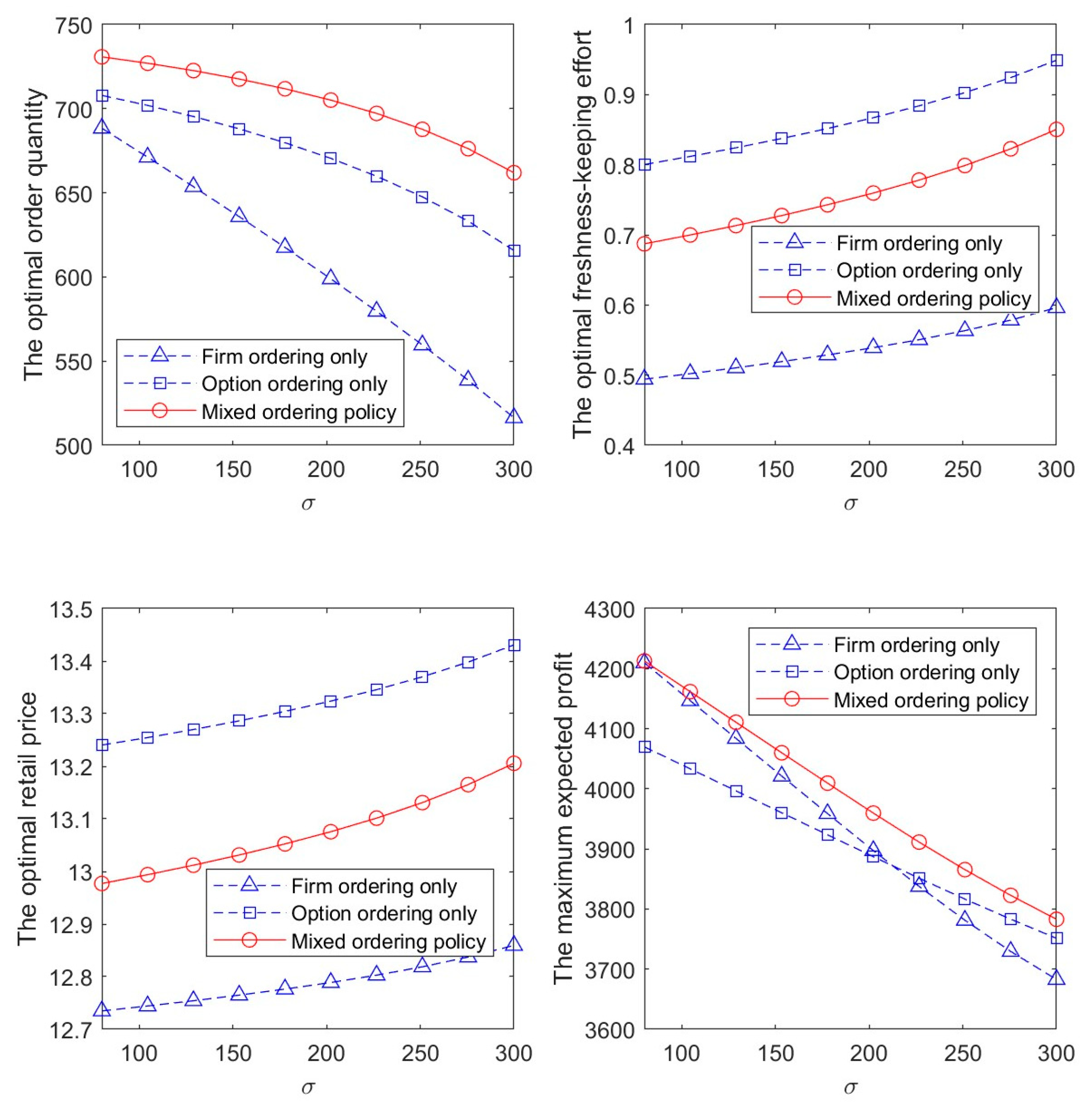
Demand risk (the variation of standard deviation ) is one of the important ways of characterizing the uncertainty of market demand. Let , , , , and , and with the change of (), we can further derive the optimal decisions of a retailer under different market demand risk conditions, thereby providing corresponding management insights.
Figure 1 describes the effects on the optimal retailer decision and maximum expected profit when facing different demand risks under two single ordering policies (firm ordering only and option ordering only) and in the case of a mixed ordering policy. By analyzing Figure 1, Remark 1–2 can be concluded.
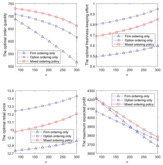
Figure 1.
The figure shows the effects of different demand risks on the optimal decisions and maximum expected profit of the retailer.
Remark 1.
The optimal order quantity for the retailer is a decreasing function of market demand risk, and the optimal order quantity when using a mixed ordering policy is greater than the optimal order quantity for two single ordering policies.
From Figure 1, with increasing demand risk, the retailer will gradually reduce their order quantities. This is contrary to the research conclusions of Wang and Chen [56]. This is because Wang and Chen [56] did not consider the existence of spot markets. In this study, when the market risk is high and there is a spot market available for replenishment to deal with uncertain demand risks, the retailer will choose to bear higher spot purchase costs instead of ordering more to deal with market demand uncertainty risks.
Remark 2.
Optimal freshness-keeping efforts and optimal retail price are both increasing functions of market demand risk.
From Figure 1, when demand risk is high, the retailer will undertake greater freshness-keeping efforts to enhance the freshness levels of fresh produce in order to increase market demand; due to the significant increase in the freshness-keeping cost and spot purchase cost for the retailer, the retailer will raise the optimal retail price to ensure their profit levels.
Result 4.
The retailer’s maximum expected profit is a decreasing function of demand risk. The relationship of the maximum expected profit between firm ordering only and option ordering only depends on demand risk, i.e., when demand risk is low, firm ordering is better than option ordering; when demand risk is high, option ordering is better than firm ordering. When all three ordering policies are available, the optimal ordering policy for the retailer is a mixed ordering policy.
According to Remark 1–2, an increase in demand risk will lead to a decrease in order quantity, an increase in order cost, and an increase in retail price. All of these factors will reduce the retailer’s expected profits. When demand risk is low, the main role of a mixed ordering policy is to reduce order cost, and at this time, the firm ordering part of a mixed ordering policy plays a role; when market risk is relatively high, the main role of mixed ordering is to reduce market risk, and at this time, the option ordering part plays a role. Compared to option ordering only, mixed ordering can reduce ordering cost; compared to firm ordering only, mixed ordering can increase supply flexibility and effectively reduce losses due to market uncertainty risks. Therefore, the optimal ordering policy for the retailer is that of mixed ordering.
6.2. Effects of Contract Parameters
- (1)
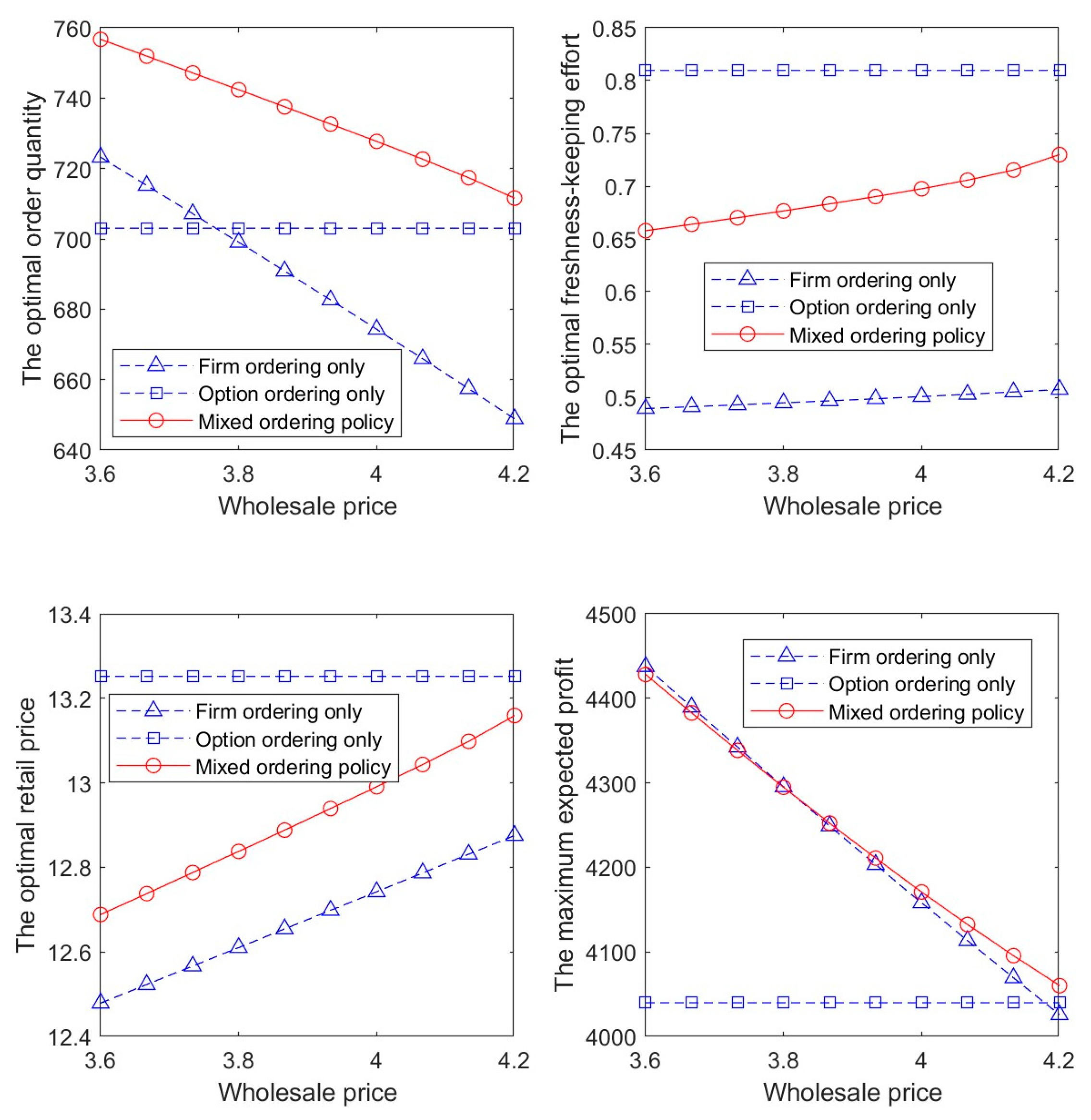
- Effects of wholesale price
Let , , , , and ; with the change of (), the effects of wholesale prices on optimal retailer decisions and maximum expected profit are shown in Figure 2.

Figure 2.
The figure shows the effects of wholesale price changes on optimal decisions and maximum expected profits in relation to the retailer.
Figure 2 describes the effects on the retailer’s optimal decisions and maximum expected profit when the wholesale price changes in the case of two single ordering policies (firm ordering only and option ordering only) and in the case of a mixed ordering policy. By analyzing Figure 2, Remark 3 can be concluded.
Remark 3.
In the case of a mixed ordering policy and a firm ordering policy, the optimal total order quantity and maximum expected profit of the retailer are decreasing functions of the wholesale price, and the optimal freshness-keeping effort and retail price are increasing functions of the wholesale price.
From Figure 2, with the increase in wholesale price, the retailer’s ordering costs for firm ordering only and for the firm ordering part, which makes up the bulk of the mixed ordering policy, increase significantly; therefore, the retailer reduces the ordered quantity; higher ordering costs will prompt the retailer to put more effort into freshness-keeping to reduce freshness loss; therefore, retailers have to raise retail prices to maintain their profit levels. However, reduced ordering quantities, increased freshness-keeping costs, and increased retail prices will all lead to a decrease in the expected profits of the retailer.
- (2)
- Effects of option price
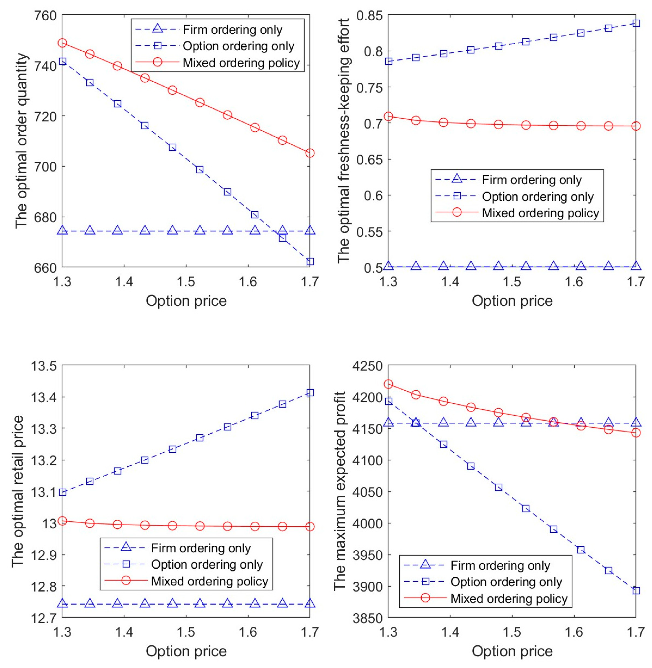
Let , , , , and ; with the change of (), the effects of option price on the optimal retailer decisions and maximum expected profit are shown in Figure 3.
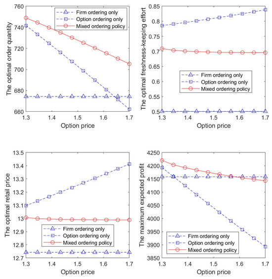
Figure 3.
The figure shows the effects of option price changes on optimal decisions and maximum expected profits in relation to the retailer.
Figure 3 describes the effects on the retailer’s optimal decisions and maximum expected profit when the option price changes in the case of two single ordering policies (firm ordering only and option ordering only) and in the case of a mixed ordering policy. By analyzing Figure 3, Remark 4 can be concluded.
Remark 4.
In the case of a mixed ordering policy and option ordering policy, the optimal total order quantity and maximum expected profit of the retailer are decreasing functions of the option price; in the case of a mixed ordering policy, the optimal freshness-keeping effort and retail price are decreasing functions of the option price, whereas the optimal freshness-keeping effort and retail price are increasing functions of the option price in the case of an option ordering policy.
From Figure 3, with the increase in option price, the retailer’s ordering costs for the case of option ordering only and for the option ordering part, which makes up of the mixed ordering policy, increase significantly. The retailer who only adheres to option ordering will reduce their order quantity and undertake greater freshness-keeping efforts to reduce losses due to spoilage, and this increased cost will force the retailer to raise retail prices, leading to a decrease in expected profits. The retailer who uses mixed ordering will reduce the option ordering part in favor of increasing the firm ordering part to reduce the total order quantity. The increase in the firm ordering part will decrease the total order cost, thereby slightly reducing the level of effort in terms of freshness-keeping. Therefore, the retailer will slightly lower their retail price to stimulate market demand. However, a decrease in order quantity will increase the probability of the retailer going to a spot market for high-cost replenishment, and the decrease in freshness level will also lead to a decrease in the retailer’s expected profit.
- (3)
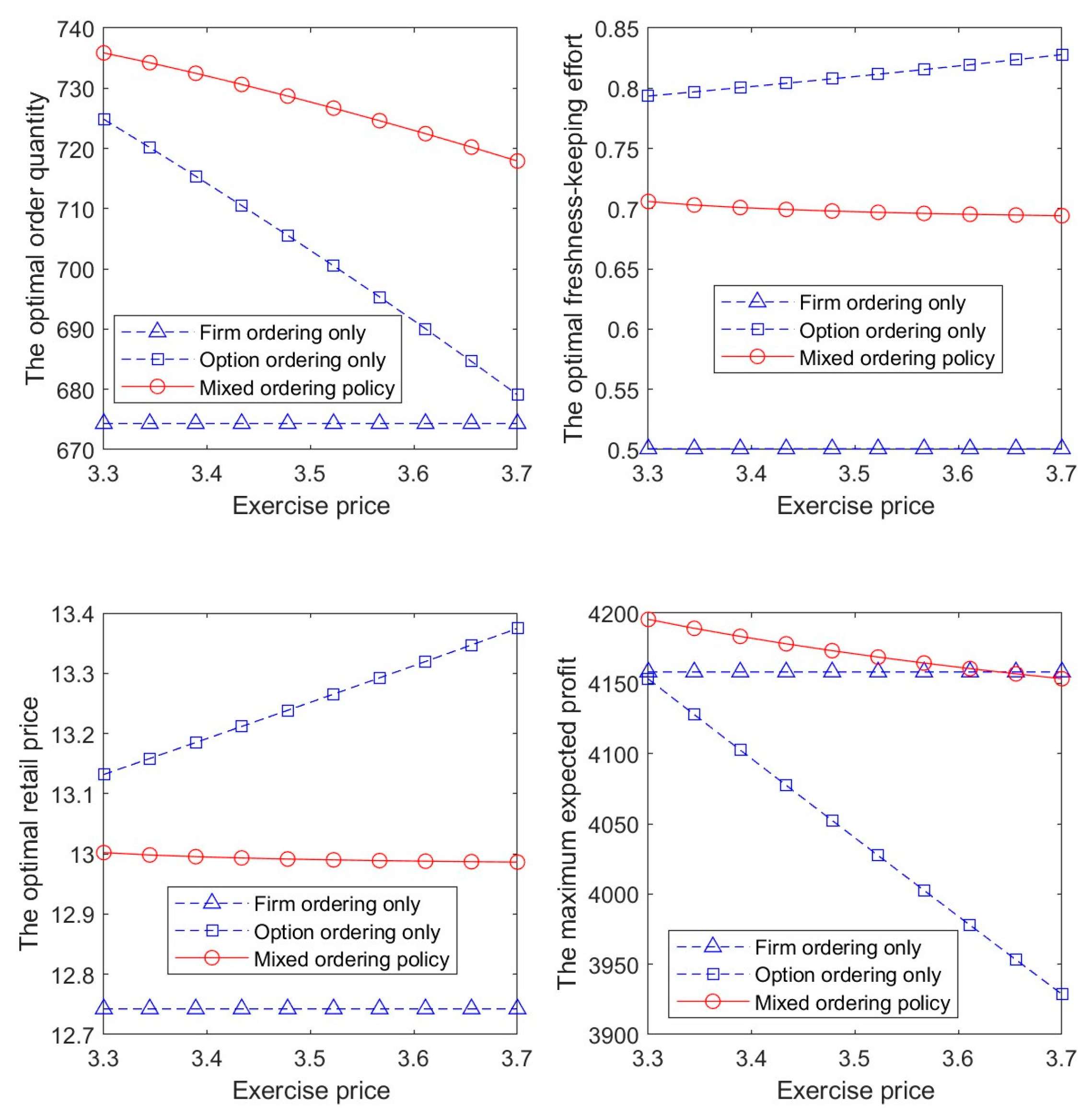
- Effects of exercise price
Let , , , , and ; with the change of (), the effects of exercise price on the retailer’s optimal decisions and maximum expected profit are shown in Figure 4.
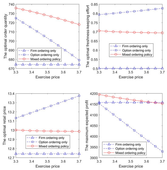
Figure 4.
The figure shows the effects of exercise price changes on optimal decisions and maximum expected profits in relation to the retailer.
Figure 4 describes the effects on the retailer’s optimal decisions and maximum expected profit when the exercise price changes in the case of two single ordering policies (firm ordering only and option ordering only) and in the case of a mixed ordering policy. By analyzing Figure 4, Remark 5 can be concluded.
Remark 5.
In the case of a mixed ordering policy and option ordering policy, the optimal total order quantity and maximum expected profit of the retailer are decreasing functions of the exercise price; in the case of a mixed ordering policy, the optimal freshness-keeping effort and retail price are decreasing functions of the exercise price, whereas the optimal freshness-keeping effort and retail price are increasing functions of the exercise price in the case of an option ordering policy.
The reasons for Remark 5 are the same as for Remark 4.
6.3. Effects of Exogenous Parameter
- (1)
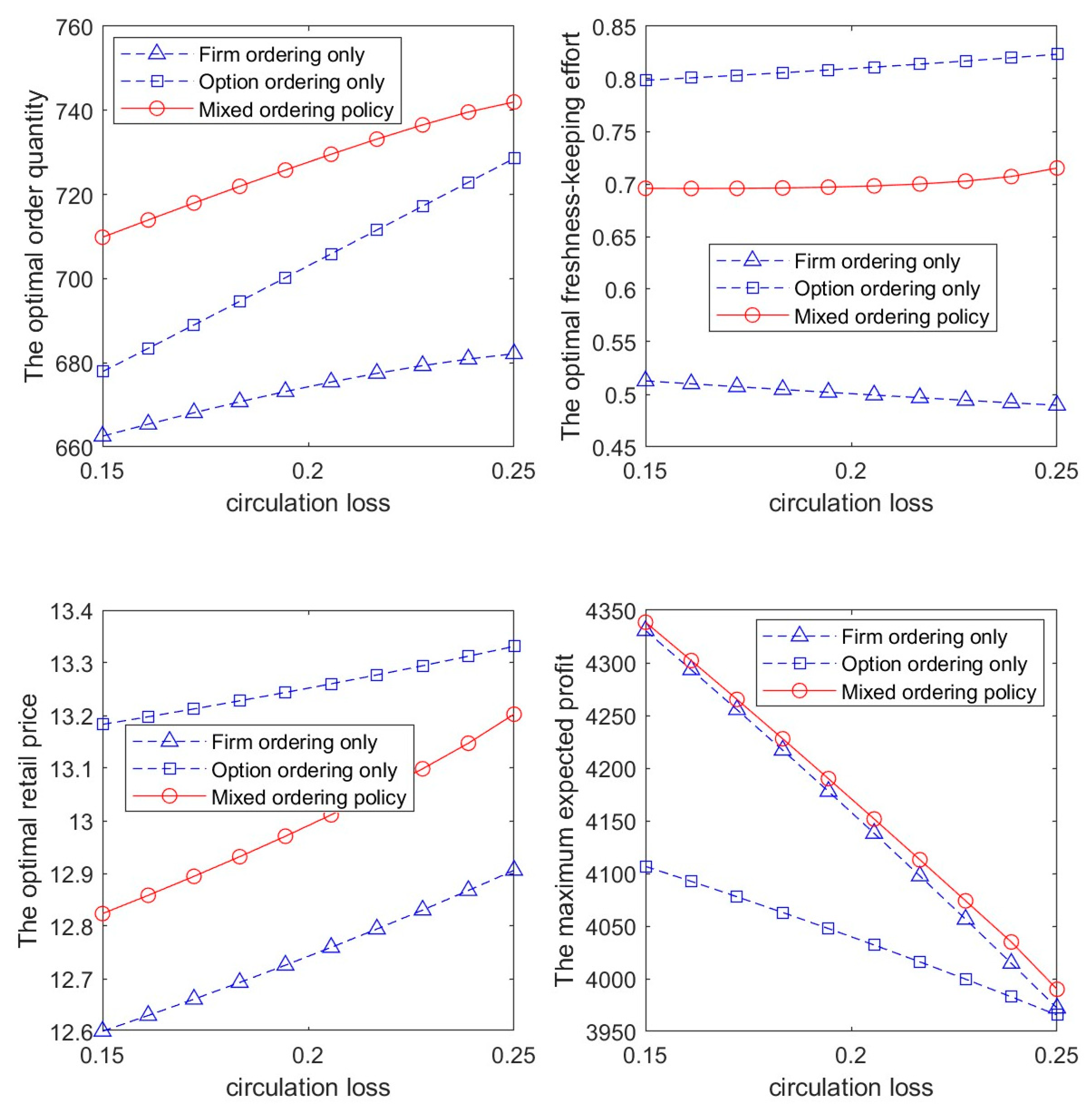
- Effects of circulation losses
Let , , , and ; with the change of (), the effects of circulation losses on the retailer’s optimal decisions and maximum expected profit are shown in Figure 5.
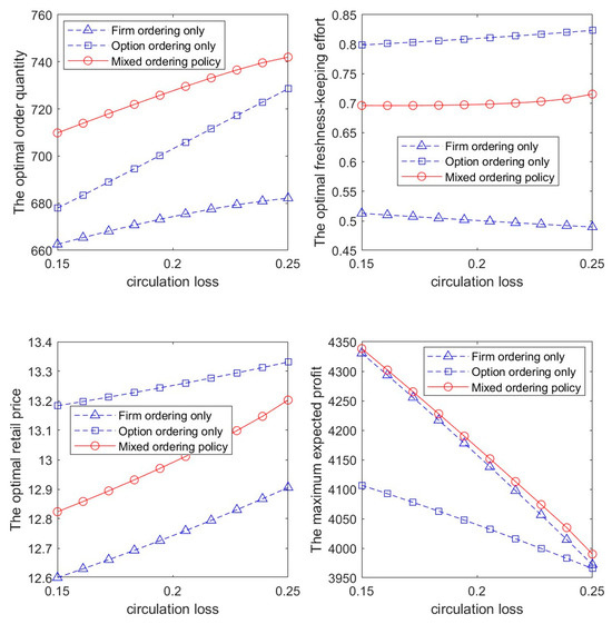
Figure 5.
The figure shows the effects of different circulation losses on the optimal decisions and maximum expected profit in relation to the retailer.
Figure 5 describes the effects on the retailer’s optimal decisions and maximum expected profit when facing different circulation losses in the case of two single ordering policies (firm ordering only and option ordering only) and in the case of mixed ordering policy. By analyzing Figure 5, Remark 6 can be concluded.
Remark 6.
The optimal total order quantity and optimal retail price of the retailer are increasing functions of circulation losses, while the maximum expected profit is a decreasing function of circulation losses. Freshness-keeping effort is an increasing function of circulation losses in the case of mixed ordering and option ordering only policies, and freshness-keeping effort is a decreasing function of circulation losses in the case of a firm ordering only policy.
From Figure 5, regardless of which ordering policy is chosen, with the market demand unchanged and increasing circulation losses, the retailer must increase their order quantity to meet market demand, and the retailer’s ordering cost will increase times. Therefore, the retailer will raise retail prices to compensate for the profit losses caused by the increase in costs.
With increasing circulation losses, for a policy with relatively low order cost, as in firm ordering only, the retailer will reduce freshness-keeping efforts; however, a policy with relatively high order costs, as in the case of option ordering only, will prompt the retailer to increase freshness-keeping efforts to reduce losses. The increase in retail price will reduce market demand, thereby reducing the retailer’s expected profit.
- (2)
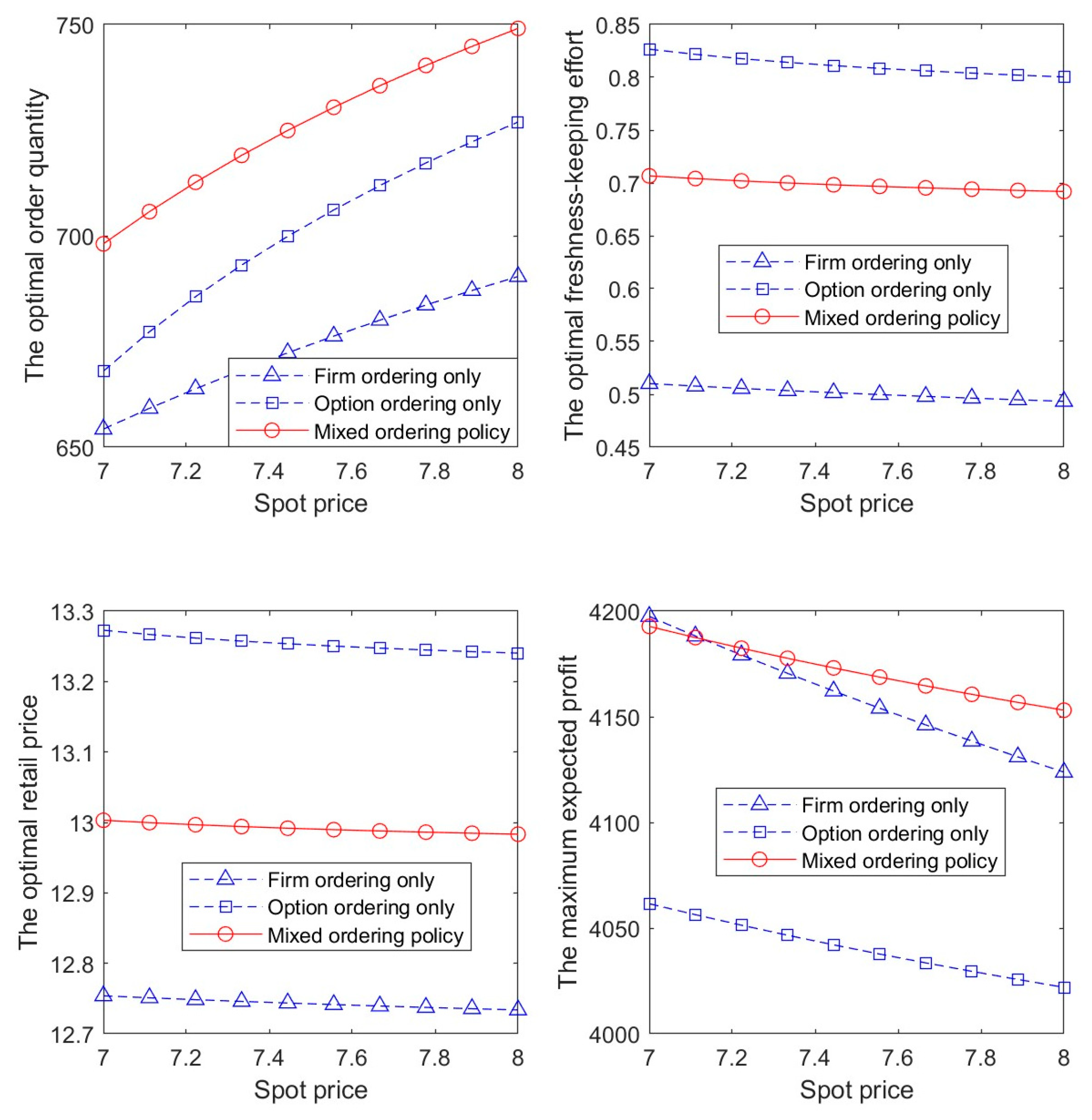
- Effects of spot price
Let , , , and ; with the change of (), the effects of spot price on the retailer’s optimal decisions and maximum expected profit are shown in Figure 6.
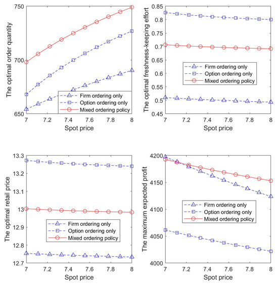
Figure 6.
The figure shows the effects of spot price changes on the optimal decisions and maximum expected profits of a retailer.
Figure 6 describes the effects on the retailer’s optimal decisions and maximum expected profit when spot price changes occur in the case of two single ordering policies (firm ordering only and option ordering only) and in the case of a mixed ordering policy. By analyzing Figure 6, Remark 7 can be concluded.
Remark 7.
The retailer’s optimal total order quantity is an increasing function of the spot price, while the optimal freshness-keeping effort, optimal retail price, and maximum expected profit are decreasing functions of the spot price.
From Figure 6, the spot price is generally higher than the sum of the ordering and freshness-keeping costs. As the spot price rises, retailers often increase their order quantity from the supplier to hedge against the risk of rising spot market prices in order to meet market demand and avoid additional cost losses from spot purchases. The spot price does not directly affect the retailer’s freshness-keeping decisions, but the increase in ordering cost due to increased order quantity forces the retailer to reduce their freshness-keeping efforts. In order to sell more fresh produce inventory, the retailer will slightly reduce the retail price to stimulate market demand. However, higher inventory, slightly lower retail price, and higher spot purchase costs will all lead to a decrease in the retailer’s expected profit.
6.4. Managerial Implications
Based on the results drawn from the numerical example, the following managerial implications are proposed to help fresh produce retailers hedge market demand risk and increase their expected profits.
- (1)
- The retailer should improve the accuracy of demand risk forecasting to optimize inventory management. Market demand risk will significantly affect the retailer’s optimal decisions and expected profits. Therefore, retailers should achieve accurate forecasting of fresh produce market demand and inventory optimization based on the data of past sales, information relating to customer behaviors and preferences, and external market conditions, in order to optimize their inventory to reduce profit losses due to stockouts of fresh produce or food waste due to unsold products.
- (2)
- The retailer should adjust ordering policies dynamically according to the external environment. Firstly, retailers should select the supplier that offers quantity flexibility contracts when ordering to obtain the ability to hedge market demand risk, such as the option contracts studied in this paper. Secondly, retailers should choose their ordering policy more accurately according to the prediction of the market demand risk, such as that shown in Result 4: when the supplier only offers a single ordering policy and the demand risk is low, the retailer should choose a wholesale price contract with lower ordering costs; when the demand risk is higher, the retailer should choose quantity flexibility contracts that can hedge the risk. Thirdly, the retailer should also consider the impact of spot markets on their optimal decisions when ordering.
- (3)
- The retailer should undertake moderate freshness-keeping efforts in relation to their fresh produce to increase expected profit. Freshness-keeping efforts are an important means of ensuring the freshness of fresh produce, reducing circulation losses, and increasing the expected profits of the retailer. However, due to the typical characteristics of fresh produce and the high cost of freshness-keeping efforts, retailers should weigh the extent to which the freshness-keeping costs increase marginal profit in order to maximize their expected profit.
7. Conclusions and Discussion
From the perspective of the double losses of fresh produce and retailers replenishing from spot markets, this article constructs the ordering, pricing, and freshness-keeping decisions in the case of single ordering policies and mixed ordering policies based on option contracts and analyzes the effects of relevant parameters on the optimal decisions and maximum expected profit. The main conclusions include the following:
- (1)
- Under the different retailer ordering policies, there are unique optimal pricing, ordering, and freshness-keeping decisions, but there is no joint decision. A fresh produce retailer can develop optimal pricing, ordering, and freshness-keeping decisions, respectively to maximize expected profit and satisfy market demand by using different ordering policies.
- (2)
- The retailer’s optimal order quantity in a mixed ordering policy is greater than that of each of the two single ordering policies; the retailer’s optimal order quantity is a decreasing function of demand risk and contract parameters, and an increasing function of circulation losses and spot price. The retailer should adopt a mixed ordering policy to achieve a higher optimal total ordering quantity, while also paying attention to the impact of factors such as demand risk, contract parameters, circulation losses, and spot prices on the ordering quantity in order to flexibly adjust the ordering quantity, effectively manage inventory risk, and enhance market competitiveness.
- (3)
- The retailer’s optimal retail price in the case of a mixed ordering policy is lower than that of option ordering only and higher than that of firm ordering only; the retailer’s optimal retail price is an increasing function of demand risk and circulation losses, and a decreasing function of spot price. A mixed ordering policy can take into account the cost advantages of a firm ordering policy and the flexibility of an option ordering policy, while also paying attention to external factors, such as demand risks, circulation losses, and spot prices, in order to improve the adaptability and market competitiveness of pricing strategies, ensuring the optimal balance between risk management and cost control.
- (4)
- Optimal retailer freshness-keeping efforts in the case of a mixed ordering policy is lower than that of option ordering only and higher than that of firm ordering only; optimal retailer freshness-keeping is an increasing function of demand risk and circulation losses, and a decreasing function of spot price. The retailer should adjust their level of freshness-keeping effort according to different ordering policies to ensure a balance between the flexibility in an options ordering policy and the cost advantages in a firm ordering policy. At the same time, sensitivity to demand risk should be increased, freshness-keeping efforts should be strengthened to cope with uncertainty, and freshness-keeping effort inputs should be moderately reduced when spot prices are high to optimize cost-effectiveness and risk management.
- (5)
- The retailer’s maximum expected profit is a decreasing function of demand risk, contract parameters, circulation losses, and spot price. If the supplier only offers a single ordering policy, when market demand risk is low, firm ordering only is better than option ordering only; when market demand risk is high, option ordering only is better than firm ordering only. If the supplier offers both a single ordering policy and a mixed ordering policy, the optimal ordering policy for the retailer is a mixed ordering policy. When pursuing maximum expected profit, the retailer should fully consider key factors such as demand risk, contract parameters, circulation losses, and spot market price, and flexibly adjust their ordering policies accordingly.
- (6)
- Compared to the situation where replenishment cannot be carried out using spot markets, the presence of spot markets will affect the retailer’s ordering, pricing, and freshness-keeping decisions, while weakening the role of option contracts in managing supply chain risks; the greater the market demand risk, the more significant the role of the spot market. Spot markets provide additional supply channels and price references for the retailer; therefore, the retailer should closely monitor spot price dynamics and incorporate them as part of their supply chain risk management strategy to enhance market adaptability and competitiveness.
Further research can be expanded from the following perspectives. First, this study investigates the management decisions of fresh produce retailers when there is a single period and a single channel, and subsequent research can be extended to multiple periods and dual channels. Second, subsequent research can be conducted on the production decisions of fresh produce suppliers facing random yield and supply chain coordination strategies. Third, this study assumes that the retailer is risk-neutral, and subsequent studies can investigate some irrational retailer decision-making behaviors through a more realistic theoretical model based on different retailer risk attitudes.
Author Contributions
Conceptualization, D.J. and C.W.; methodology, D.J. and C.W.; software, D.J. and X.C.; formal analysis, D.J. and X.C.; investigation, D.J. and X.C.; writing—original draft preparation, D.J.; writing—review and editing, X.C.; supervision, C.W.; funding acquisition, C.W. All authors have read and agreed to the published version of the manuscript.
Funding
This research was partly supported by the National Natural Science Foundation of China (No. 71972136), and Sichuan Science and Technology Program (No. 2022JDTD0022).
Institutional Review Board Statement
Not applicable.
Informed Consent Statement
Not applicable.
Data Availability Statement
Data are contained within the article.
Acknowledgments
The authors would like to thank the editor and the anonymous reviewers for their valuable comments.
Conflicts of Interest
The authors declare that there are no conflicts of interest regarding the publication of this paper.
Appendix A
Proof of Lemma 1.
For given , , . Then, for given , is concave with respect to . Let , the retailer’s optimal retail price can be obtained. This completes the proof. □
Proof of Lemma 2.
For , , . According to Assumption 3, it can be known that ; . Therefore, obviously, there is . Then, for , is concave with respect to , so there exists a unique optimal freshness-keeping effort that maximizes the expected profit of the retailer. Let , the retailer’s optimal freshness-keeping effort satisfies Equation (6) and can be obtained. This completes the proof. □
Proof of Lemma 3.
For , , . Then, for , is concave with respect to . Therefore, there exists a unique optimal firm order quantity that maximizes the expected profit of the retailer, and , where is the unique on that satisfies . This completes the proof. □
Proof of Proposition 1.
According to Lemma 3, let , can be obtained, i.e., is the unique on that satisfies . Therefore, the retailer’s optimal order quantity at firm ordering only is . This completes the proof. □
Proof of Lemma 4.
The proof of Lemma 4 is similar to the proof of Lemma 1. □
Proof of Lemma 5.
The proof of Lemma 5 is similar to the proof of Lemma 2. □
Proof of Lemma 6.
The proof of Lemma 6 is similar to the proof of Lemma 3. □
Proof of Proposition 2.
According to Lemma 3, let , can be obtained, i.e., is the unique on that satisfies . Therefore, the retailer’s optimal order quantity at option ordering only is . This completes the proof. □
Proof of Lemma 7.
The proof of Lemma 7 is similar to the proof of Lemma 1. □
Proof of Lemma 8.
The proof of Lemma 8 is similar to the proof of Lemma 2. □
Proof of Lemma 9.
For , , ; , . Additionally, , , . When , . Then, the Hessian matrix is a negative definite. Then, for , is the joint concave function with respect to and . Therefore, there exists a unique optimal option order quantity and total order quantity that maximizes the retailer’s expected profit, and , where is the unique on that satisfies . This completes the proof. □
Proof of Proposition 3.
Substitute and into , we can get ; . According to Lemma 3, let , ; let , . Substitute the latter equation into the former, can be obtained, namely, is the unique on that satisfies . This completes the proof. □
References
- Cai, X.Q.; Chen, J.; Xiao, Y.B.; Xu, X.L. Optimization and Coordination of Fresh Product Supply Chains with Freshness-Keeping Effort. Prod. Oper. Manag. 2010, 19, 261–278. [Google Scholar]
- Qin, Y.Y.; Wang, J.J.; Wei, C.M. Joint pricing and inventory control for fresh produce and foods with quality and physical quantity deteriorating simultaneously. Int. J. Prod. Econ. 2014, 152, 42–48. [Google Scholar] [CrossRef]
- Yang, C.Y.; Feng, Y.H.; Whinston, A. Dynamic Pricing and Information Disclosure for Fresh Produce: An Artificial Intelligence Approach. Prod. Oper. Manag. 2022, 31, 155–171. [Google Scholar] [CrossRef]
- Wang, C.; Chen, X. Option pricing and coordination in the fresh produce supply chain with portfolio contracts. Ann. Oper. Res. 2017, 248, 471–491. [Google Scholar] [CrossRef]
- Gu, B.J.; Fu, Y.F.; Ye, J. Joint optimization and coordination of fresh-product supply chains with quality-improvement effort and fresh-keeping effort. Qual. Technol. Quant. Manag. 2021, 18, 20–38. [Google Scholar] [CrossRef]
- Wang, C.; Chen, X. Fresh produce price-sitting newsvendor with bidirectional option contracts. J. Ind. Manag. Optim. 2022, 18, 1979–2000. [Google Scholar] [CrossRef]
- Herbon, A.; Khmelnitsky, E. Optimal dynamic pricing and ordering of a perishable product under additive effects of price and time on demand. Eur. J. Oper. Res. 2017, 260, 546–556. [Google Scholar] [CrossRef]
- Jin, C.Y.; Levi, R.; Liang, Q.; Renegar, N.; Springs, S.; Zhou, J.H.; Zhou, W.H. Testing at the Source: Analytics-Enabled Risk-Based Sampling of Food Supply Chains in China. Manag. Sci. 2021, 67, 2985–2996. [Google Scholar] [CrossRef]
- Zhao, Y.X.; Choi, T.M.; Cheng, T.C.E.; Sethi, S.P.; Wang, S.Y. Buyback contracts with price-dependent demands: Effects of demand uncertainty. Eur. J. Oper. Res. 2014, 239, 663–673. [Google Scholar] [CrossRef]
- Hu, B.Y.; Feng, Y. Optimization and coordination of supply chain with revenue sharing contracts and service requirement under supply and demand uncertainty. Int. J. Prod. Econ. 2017, 183, 185–193. [Google Scholar] [CrossRef]
- Zheng, Q.; Zhou, L.; Fan, T.J.; Ieromonachou, P. Joint procurement and pricing of fresh produce for multiple retailers with a quantity discount contract. Transp. Res. Part E-Logist. Transp. Rev. 2019, 130, 16–36. [Google Scholar] [CrossRef]
- Yang, L.; Tang, R.H.; Chen, K.B. Call, put and bidirectional option contracts in agricultural supply chains with sales effort. Appl. Math. Model. 2017, 47, 1–16. [Google Scholar] [CrossRef]
- Wang, C.; Chen, J.; Chen, X. Pricing and order decisions with option contracts in the presence of customer returns. Int. J. Prod. Econ. 2017, 193, 422–436. [Google Scholar] [CrossRef]
- Chen, X.; Wan, N.N.; Wang, X.J. Flexibility and coordination in a supply chain with bidirectional option contracts and service requirement. Int. J. Prod. Econ. 2017, 193, 183–192. [Google Scholar] [CrossRef]
- Biswas, I.; Avittathur, B. Channel coordination using options contract under simultaneous price and inventory competition. Transp. Res. Part E-Logist. Transp. Rev. 2019, 123, 45–60. [Google Scholar] [CrossRef]
- Zhuo, W.Y.; Shao, L.S.; Yang, H.L. Mean-standard deviation analysis of option contracts in a two-echelon supply chain. Eur. J. Oper. Res. 2018, 271, 535–547. [Google Scholar] [CrossRef]
- Blackburn, J.; Scudder, G. Supply Chain Strategies for Perishable Products: The Case of Fresh Produce. Prod. Oper. Manag. 2009, 18, 129–137. [Google Scholar] [CrossRef]
- Cai, X.Q.; Feng, Y.; Li, Y.J.; Shi, D. Optimal pricing policy for a deteriorating product by dynamic tracking control. Int. J. Prod. Res. 2013, 51, 2491–2504. [Google Scholar] [CrossRef]
- Albrecht, W.; Steinrucke, M. Coordinating continuous-time distribution and sales planning of perishable goods with quality grades. Int. J. Prod. Res. 2018, 56, 2646–2665. [Google Scholar] [CrossRef]
- Chen, X.; Wu, S.Y.; Wang, X.J.; Li, D. Optimal pricing strategy for the perishable food supply chain. Int. J. Prod. Res. 2019, 57, 2755–2768. [Google Scholar] [CrossRef]
- Xu, C.; Fan, T.J.; Zheng, Q.; Song, Y. Contract selection for fresh produce suppliers cooperating with a platform under a markdown-pricing policy. Int. J. Prod. Res. 2021, 61, 3756–3780. [Google Scholar] [CrossRef]
- Mamoudan, M.M.; MohammadNazari, Z.; Ostadi, A.; Esfahbodi, A. Food products pricing theory with application of machine learning and game theory approach. Int. J. Prod. Res. 2022, 1–21. [Google Scholar] [CrossRef]
- Rabbani, M.; Zia, N.P.; Rafiei, H. Joint optimal dynamic pricing and replenishment policies for items with simultaneous quality and physical quantity deterioration. Appl. Math. Comput. 2016, 287, 149–160. [Google Scholar] [CrossRef]
- Rahdar, M.; Nookabadi, A.S. Coordination mechanism for a deteriorating item in a two-level supply chain system. Appl. Math. Model. 2014, 38, 2884–2900. [Google Scholar] [CrossRef]
- Zhang, J.X.; Liu, G.W.; Zhang, Q.; Bai, Z.Y. Coordinating a supply chain for deteriorating items with a revenue sharing and cooperative investment contract. Omega-Int. J. Manag. Sci. 2015, 56, 37–49. [Google Scholar] [CrossRef]
- Panda, S.; Modak, N.M.; Cardenas-Barron, L.E. Coordination and benefit sharing in a three-echelon distribution channel with deteriorating product. Comput. Ind. Eng. 2017, 113, 630–645. [Google Scholar] [CrossRef]
- Dye, C.Y.; Hsieh, T.P. An optimal replenishment policy for deteriorating items with effective investment in preservation technology. Eur. J. Oper. Res. 2012, 218, 106–112. [Google Scholar] [CrossRef]
- Liu, M.L.; Dan, B.; Zhang, S.G.; Ma, S.X. Information sharing in an E-tailing supply chain for fresh produce with freshness-keeping effort and value-added service. Eur. J. Oper. Res. 2021, 290, 572–584. [Google Scholar] [CrossRef]
- Zheng, Q.; Ieromonachou, P.; Fan, T.J.; Zhou, L. Supply chain contracting coordination for fresh products with fresh-keeping effort. Ind. Manag. Data Syst. 2017, 117, 538–559. [Google Scholar] [CrossRef]
- Mohammadi, H.; Ghazanfari, M.; Pishvaee, M.S.; Teimoury, E. Fresh-product supply chain coordination and waste reduction using a revenue-and-preservation-technology-investment-sharing contract: A real-life case study. J. Clean. Prod. 2019, 213, 262–282. [Google Scholar] [CrossRef]
- Cai, X.Q.; Chen, J.; Xiao, Y.B.; Xu, X.L.; Yu, G. Fresh-product supply chain management with logistics outsourcing. Omega 2013, 41, 752–765. [Google Scholar] [CrossRef]
- Wu, Q.; Mu, Y.P.; Feng, Y. Coordinating contracts for fresh product outsourcing logistics channels with power structures. Int. J. Prod. Econ. 2015, 160, 94–105. [Google Scholar] [CrossRef]
- Yu, Y.L.; Xiao, T.J. Pricing and cold-chain service level decisions in a fresh agri-products supply chain with logistics outsourcing. Comput. Ind. Eng. 2017, 111, 56–66. [Google Scholar] [CrossRef]
- Song, Z.L.; He, S.W. Contract coordination of new fresh produce three-layer supply chain. Ind. Manag. Data Syst. 2019, 119, 148–169. [Google Scholar] [CrossRef]
- Yu, Y.L.; Xiao, T.J.; Feng, Z.W. Price and cold-chain service decisions versus integration in a fresh agri-product supply chain with competing retailers. Ann. Oper. Res. 2020, 287, 465–493. [Google Scholar] [CrossRef]
- Gomez-Padilla, A.; Mishina, T. Supply contract with options. Int. J. Prod. Econ. 2009, 122, 312–318. [Google Scholar] [CrossRef]
- Zhao, Y.X.; Wang, S.Y.; Cheng, T.C.E.; Yang, X.Q.; Huang, Z.M. Coordination of supply chains by option contracts: A cooperative game theory approach. Eur. J. Oper. Res. 2010, 207, 668–675. [Google Scholar] [CrossRef]
- Zhao, Y.X.; Ma, L.J.; Xie, G.; Cheng, T.C.E. Coordination of supply chains with bidirectional option contracts. Eur. J. Oper. Res. 2013, 229, 375–381. [Google Scholar] [CrossRef]
- Liu, Z.Y.; Chen, L.H.; Li, L.; Zhai, X. Risk hedging in a supply chain: Option vs. price discount. Int. J. Prod. Econ. 2014, 151, 112–120. [Google Scholar] [CrossRef]
- Fu, X.; Dong, M.; Han, G.H. Coordinating a trust-embedded two-tier supply chain by options with multiple transaction periods. Int. J. Prod. Res. 2017, 55, 2068–2082. [Google Scholar] [CrossRef]
- Chen, X.; Hao, G.; Li, L. Channel coordination with a loss-averse retailer and option contracts. Int. J. Prod. Econ. 2014, 150, 52–57. [Google Scholar] [CrossRef]
- Basu, P.; Liu, Q.D.; Stallaert, J. Supply chain management using put option contracts with information asymmetry. Int. J. Prod. Res. 2019, 57, 1772–1796. [Google Scholar] [CrossRef]
- Xu, X.S.; Chan, F.T.S.; Chan, C.K. Optimal option purchase decision of a loss-averse retailer under emergent replenishment. Int. J. Prod. Res. 2019, 57, 4594–4620. [Google Scholar] [CrossRef]
- Fan, Y.H.; Feng, Y.; Shou, Y.Y. A risk-averse and buyer-led supply chain under option contract: CVaR minimization and channel coordination. Int. J. Prod. Econ. 2020, 219, 66–81. [Google Scholar] [CrossRef]
- Liu, Z.Y.; Hua, S.Y.; Zhai, X. Supply chain coordination with risk-averse retailer and option contract: Supplier-led vs. Retailer-led. Int. J. Prod. Econ. 2020, 223, 107518. [Google Scholar] [CrossRef]
- Luo, J.R.; Chen, X. Risk hedging via option contracts in a random yield supply chain. Ann. Oper. Res. 2017, 257, 697–719. [Google Scholar] [CrossRef]
- Luo, J.R.; Zhang, X.L.; Wang, C. Using put option contracts in supply chains to manage demand and supply uncertainty. Ind. Manag. Data Syst. 2018, 118, 1477–1497. [Google Scholar] [CrossRef]
- Luo, J.R.; Chen, X.; Wang, C.; Zhang, G.X. Bidirectional options in random yield supply chains with demand and spot price uncertainty. Ann. Oper. Res. 2021, 302, 211–230. [Google Scholar] [CrossRef]
- Fu, Q.; Zhou, S.X.; Chao, X.L.; Lee, C.Y. Combined Pricing and Portfolio Option Procurement. Prod. Oper. Manag. 2012, 21, 361–377. [Google Scholar] [CrossRef]
- Zhao, Y.X.; Choi, T.M.; Cheng, T.C.E.; Wang, S.Y. Supply option contracts with spot market and demand information updating. Eur. J. Oper. Res. 2018, 266, 1062–1071. [Google Scholar] [CrossRef]
- Wang, C.; Chen, J.; Chen, X. The impact of customer returns and bidirectional option contract on refund price and order decisions. Eur. J. Oper. Res. 2019, 274, 267–279. [Google Scholar] [CrossRef]
- Wang, C.; Chen, J.; Wang, L.L.; Luo, J.R. Supply chain coordination with put option contracts and customer returns. J. Oper. Res. Soc. 2020, 71, 1003–1019. [Google Scholar] [CrossRef]
- Wang, C.; Chen, X. Joint order and pricing decisions for fresh produce with put option contracts. J. Oper. Res. Soc. 2018, 69, 474–484. [Google Scholar] [CrossRef]
- Jia, D.; Wang, C. Option Contracts in Fresh Produce Supply Chain with Freshness-Keeping Effort. Mathematics 2022, 10, 1287. [Google Scholar] [CrossRef]
- Chen, X.; Wang, C.; Jia, D.; Bai, Y. Multi-period pricing and order decisions for fresh produce with option contracts. Ann. Oper. Res. 2023, 335, 79–110. [Google Scholar] [CrossRef]
- Wang, C.; Chen, X. Optimal ordering policy for a price-setting newsvendor with option contracts under demand uncertainty. Int. J. Prod. Res. 2015, 53, 6279–6293. [Google Scholar] [CrossRef]
- Petruzzi, N.C.; Dada, M. Pricing and the Newsvendor Problem: A Review with Extensions. Oper. Res. 1999, 47, 183–194. [Google Scholar] [CrossRef]
Disclaimer/Publisher’s Note: The statements, opinions and data contained in all publications are solely those of the individual author(s) and contributor(s) and not of MDPI and/or the editor(s). MDPI and/or the editor(s) disclaim responsibility for any injury to people or property resulting from any ideas, methods, instructions or products referred to in the content. |
© 2024 by the authors. Licensee MDPI, Basel, Switzerland. This article is an open access article distributed under the terms and conditions of the Creative Commons Attribution (CC BY) license (https://creativecommons.org/licenses/by/4.0/).