Abstract
The Northern Gulf of Mexico hosts a severe dead zone, an oxygen-depleted area spanning 1,618,000 hectares, threatening over 40% of the U.S. fishing industry and causing annual losses of USD 82 million. Using a System Dynamics (SD) approach, this study examined the Mississippi–Atchafalaya River Basin (MARB), a major contributor to hypoxia in the Gulf. A dynamic model, developed with Vensim software version 10.2.1 andexisting data, represented the physical, biological, and chemical processes leading to eutrophication and simulated dead zone formation over time. Various policies were assessed, considering natural system variability. The findings showed that focusing solely on nitrogen control reduced the dead zone but required greater intensity or managing other inputs to meet environmental goals. Runoff control policies delayed nutrient discharge but did not significantly alter long-term outcomes. Extreme condition tests highlighted the critical role of runoff dynamics, dependent on nitrogen load relative to flow volume from upstream. The model suggests interventions should not just reduce eutrophication inputs but enhance factors slowing down the process, allowing natural denitrification to override anthropogenic nitrification.
1. Introduction
Dead zones are regions in oceans and large lakes with deficient oxygen levels. These areas possess a condition known as hypoxia. Hypoxia occurs when the concentration of dissolved oxygen (D.O.) in water drops to 2 mg of O2 per liter or less. In these situations, aquatic plants and animals relocate to areas with higher oxygen levels. If the D.O. levels plummet below 0.5 mL O2 per liter, water bodies become incapable of supporting aquatic life.
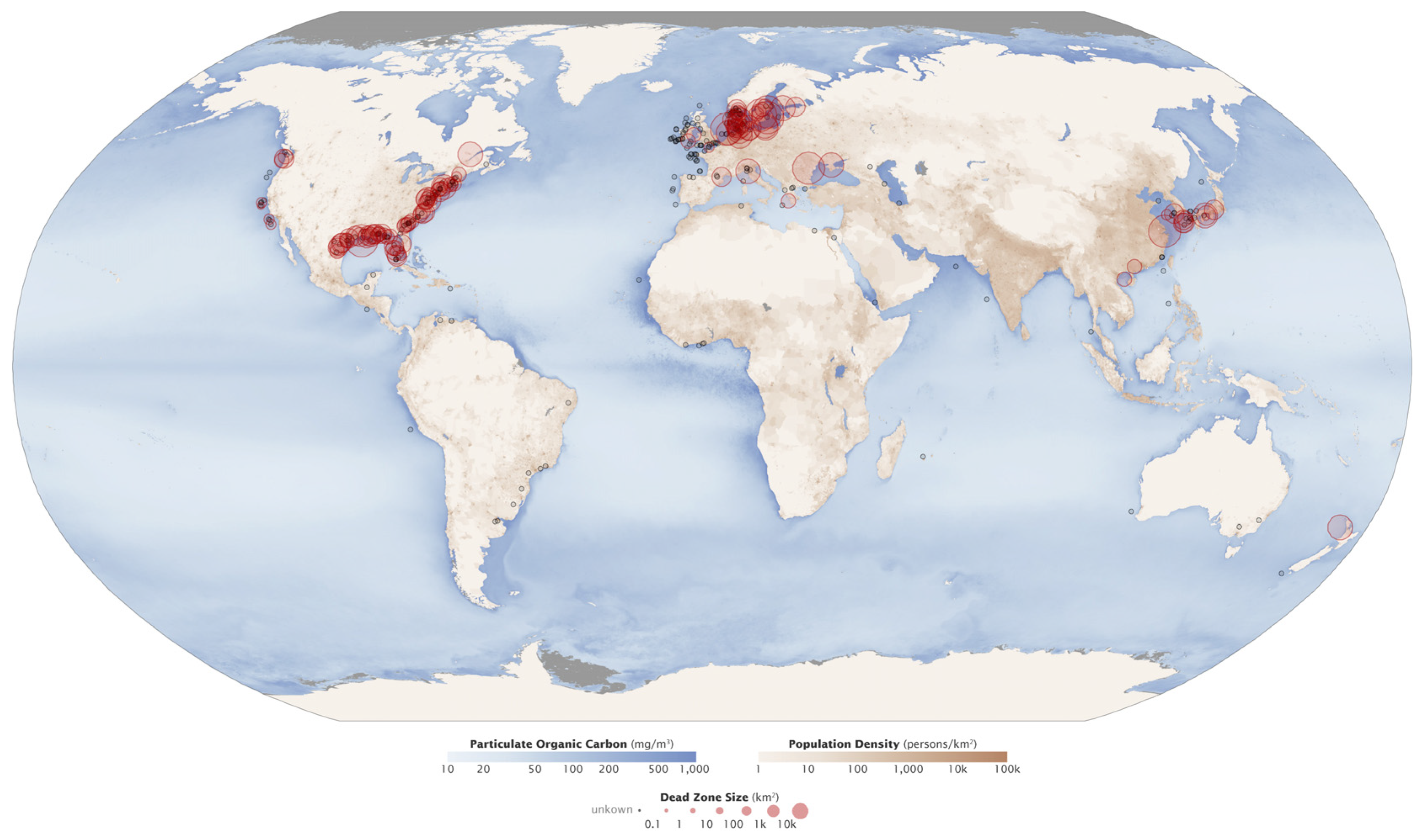
While dead zones can occur naturally [1], the most notorious recent cases have originated from man-made nutrient sources such as treatment plants, sewage, farms, or lawns [2]. In the Mississippi–Atchafalaya River Basin (MARB), many excess nutrients are released from sources such as these and are eventually transported into the Northern Gulf of Mexico (Figure 1). Algal blooms then take place, using nutrients and depleting oxygen in the water. This process is known as eutrophication and is the culprit for the creation of the dead zone found in the Gulf of Mexico [3]. Other marine hypoxic zones exist in the rest of the world (Figure 2), including the coasts of Northeast Asia, Northern Europe, the Mediterranean Sea, and others [4].

Figure 1.
Map illustrating the extent of the Mississippi–Atchafalaya River Basin and its contributing rivers [5].
This study examines interactions between sources of water and nitrogen leading to the process of eutrophication. They are two vital components in eutrophication that lead to hypoxic area emergence [6]. The interplay between the two elements was represented in this study for the specific case of the Mississippi–Atchafalaya River Basin (MARB) by implementing it in the Vensim software version 10.2.1 package. Vensim is a tool used for building, analyzing, and simulating models to understand system behavior over time. Official EPA reports and the prior literature regarding the case were used as the foundation for calibrating the model and determining its inputs with their respective proportions.
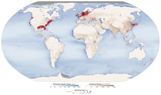
Figure 2.
Map highlighting hypoxic areas in different regions of the world. Red circles show the location and size of different aquatic dead zones as of 2008. Black dots show dead zones of unknown size [7].
Figure 2.
Map highlighting hypoxic areas in different regions of the world. Red circles show the location and size of different aquatic dead zones as of 2008. Black dots show dead zones of unknown size [7].
Our modeling approach aimed to gain insights into how nitrogen is transported via surface water and runoff in different parts of the MARB and improve managerial recommendations at different levels. System Dynamics (SD) was the modeling method used in this study. Models created using SD seek to analyze complex systems by focusing on their structure, behavior, and interactions over time. Unlike traditional modeling methods that often emphasize detailed knowledge of specific individual components, SD focuses on the broader dynamics that arise from the interactions between these components. This approach allows us to uncover and address the underlying factors contributing to systemic issues that are often overlooked in other models [8].
Models built using SD are comprised of feedback loops, stocks, and flows [9,10]. These elements represent the relationships and dependencies within a system. Feedback loops can be either reinforcing or balancing. Reinforcing loops leads to the growth or amplification of a certain effect. Balancing loops counteract change to stabilize the system. Stocks represent accumulations of resources, materials, or information. Flows are connected to stocks and determine the rates at which their accumulations change over time. These elements are used in SD to simulate interactions to provide insights into how changes in one part of a system can be the cause of outcomes elsewhere [10,11].
The utilization of the SD method allowed for the exploration of the processes leading to eutrophication and the formation of the dead zone in the Northern Gulf of Mexico with a perspective that prioritizes system-wide behavior over specific component details. This tradeoff allows us to observe and account for the interplay of factors such as nutrient runoff, water flow, and biological processes at a basin scale. This approach ultimately provided a means to understanding how policy interventions might mitigate the formation of the dead zone over extended periods.
The Vensim software version 10.2.1 successfully translates the concepts rooted in SD into a simulation that captures the interplay between the role of inputs, variables that may vary seasonally, and the effect of potential intervention policies. An initial base model was created as a control. Different scenarios were then created as the treatment groups by manipulating specific parameters of the base model. Data derived from simulating such treatments allowed a comparison of outcomes in terms of the resulting area of the dead zone in square kilometers. By observing the contrasting results of the dead zone area, we can better explain the variability in the extension of the dead zone in the Gulf of Mexico in recent years. The slightly volatile but steadily growing area of the dead zone leaves a question as to what extent is human activity the culprit for expansion or contraction in a given year (Figure 3A). The study also seeks to explain how the proportions and weights of the influences of varying amounts of water and nutrients (specifically nitrogen) act upon the system (Figure 3B). This research represents a specific application of a method that has already found use across different contexts including business, health care, and environmental modeling.
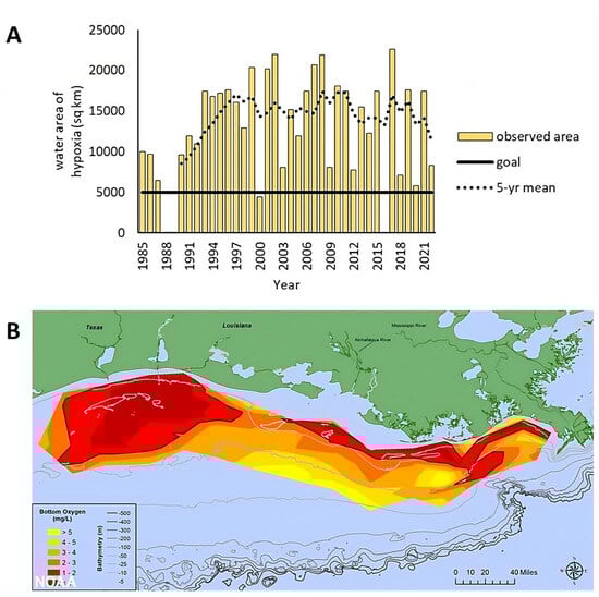
Figure 3.
Behavior over time of the Gulf of Mexico dead zone (A) (data replicated from [1]). Map of the dead zone in the Northern Gulf of Mexico (B), depicting varying oxygen concentration levels, which are inversely correlated to nitrogen loading [12].
The simulation analysis spans multiple decades—a necessary duration for observing the effects of different strategic policies beyond their immediate consequences. The subsequent sections provide a detailed breakdown of the modeling process and the application model to better understand the system dynamics ongoing within the MARB. The outcomes of the different simulations carried out are presented and the insights derived from them are each delineated in their respective segment.
2. Materials and Methods
As mentioned previously, SD represents a methodological approach and can be applied via Vensim as a simulation tool tailored for the detailed modeling of dynamic and complex systems. It can illustrate and account for the self-reinforcing mechanisms that characterize systems such as that of the MARB and the dead zone of the Gulf of Mexico. An initial change in a component of the system influences others, which in turn triggers a series of chain reactions that may either amplify or attenuate the metric sought to be modified by the initial perturbation of the system. The SD approach also observes that alterations in a system do not manifest in isolation; instead, it comprehends the inherent interdependencies within systems. Recognition of the role of delays in SD also acknowledges that many systems do not exhibit immediate reactions to perturbations. The importance of observations consistently made through time can capture the true behavior of a system and is underscored by the emphasis made on the existence of delays.
Self-regulating systems are omnipresent in societies, organizations, and nature. They are particularly observable in ecological and social systems that accumulate stocks of essential variables that are vital to a system’s operation. A form of effective SD application can be found when addressing complex environmental issues. The leverage of using SD to address problems of this nature resides in that they usually involve biological, chemical, and physical processes that are variable. Causal relationships between processes in nature are often unperceivable at a surface level. Addressing such issues will frequently demand efforts beyond isolated interventions at the localized levels. SD can inform decision-making by contributing to a more holistic understanding of the influence of their actions in a system and the interconnections within it.
Interactions within a system are expressed as feedback loops in SD. For example, hypothetically, a very adverse year where the dead zone may have caused a significant economic loss on a certain year, which may have incited an increase in efforts to control nutrient leaching from agriculture, in turn leading to higher consumer prices as a result of higher costs proceeding from regulations, exacerbating the initial economic stress that triggered the first action. Feedback loops with delays and impacts originating from different directions and variables can result in nonlinear, unforeseen behavior. In essence, feedback mechanisms’ unpredictability can give rise to unintended consequences, even when policy decisions initially appear to be rational [13].
The method used in SD is considered reliable for evaluating the control of intricate environmental systems. It has been successfully applied to agricultural development [14] and water resource management [9,15]. This method employs a framework that allows us to account for and examine the consequences of intricate dynamic interactions within a system. It encompasses the influence of feedback mechanisms, allowing the assessment of policies considering their broad systemic consequences. Systems are illustrated in SD by transcribing causal loops into stock and flow diagrams that allow for simulation via Vensim. These diagrams effectively represent the accumulations (stocks) and the rates of change (flows) integral to a system’s function.
An SD stock and flow model mimics the behavior systems via iterative step-wise mathematical integration, where variable values at a given time (t) progress with each time step and feedforward to inform model calculations at the following time (t + 1). Inputs and outputs flowed through the system and were updated for each time step. A yearly time step was used in this study. Many key processes, including nutrient runoff from agriculture, seasonal weather patterns, and the resulting algal blooms, follow significant annual cycles. The rate of recurrence of such events makes it logical to analyze and predict the system’s behavior annually.
The MARB stock and flow model created in this study (Figure 4) encompasses separate sections. The left side of the figure illustrates the subsystem of water flow, detailing how water is conveyed from the upper MARB, passing through various branches before ultimately being discharged into the Gulf. The right side represents a load of nitrogen collected at different parts of the depicted channels, acting in parallel to the left side to simulate the stocks of nitrogen being washed down until reaching the Gulf. This set of two main subsystems includes the main river channels and tributaries, capturing the complexity of water movement through different regions of the basin. It also incorporates factors such as rainfall and conveyance time of flow, providing a comprehensive view of the hydrological processes at play. By accurately representing these water flow dynamics, the model helps in understanding the temporal and spatial variations in water discharge and its impact on the downstream regions, including the Gulf of Mexico.
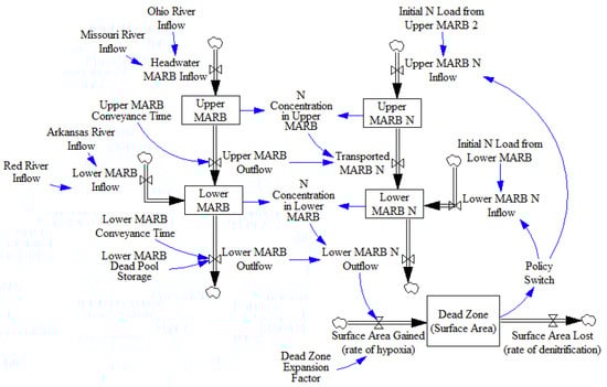
Figure 4.
Simplified sketch of Vensim base model for the MARB basin system. In the diagram, a rectangle represents a stock, while an arrow depicts the flow of either entering or leaving the stock. Blue arrows connect variables and other factors represented in simplified forms in this sketch that influence the state of the stocks and flows.
To simplify the arrangement of the streams in the model, the various channels that make up the Mississippi–Atchafalaya River Basin (MARB) have been amalgamated into two consolidated sets of stocks and flows, categorized as Upper and Lower MARB, respectively. In the model, the Upper MARB stock is composed of the headwaters of the Ohio and Missouri rivers. The Arkansas and Red rivers contribute to the Lower MARB section. This consolidation facilitates the modeling process by reducing the complexity inherent in representing each channel. A cumulative flow was assigned based on the reviewed flow regimes of the channels belonging to the upper and lower sections of the MARB, ensuring that the model accurately reflects the aggregate water movement through these segments. By grouping the channels into these two sets, the model can effectively capture the overall dynamics of water flow within the basin while maintaining a manageable level of detail for analysis and simulation purposes. This approach enables a clearer understanding of how water is distributed and transported across the MARB, ultimately impacting the discharge into the Gulf of Mexico.
The volume of flow from each of the sources is determined by the combination of two parameters. The surface area and the annual precipitation depth will determine the annual flow from a given source in the model. The surface area is a fixed value based on existing knowledge about the drainage area of each contributing stream. Precipitation can be subject to change; it may be left as a fixed average value throughout a simulation but it can also be assigned a randomized property so that it may yield a different input in every time step. For the tests conducted in the study, rainfall was held constant using the precipitation data recorded in the year 2017, which was used as a baseline.
The complete MARB management model also involves significant detail for nitrogen within the system. The concentration of nitrogen being transported along the MARB is represented on the right-hand side in Figure 4. The load of nitrogen being transported is proportional to what would need to be allocated in each of the streams to deliver the nitrogen corresponding to the average area of the dead zone since it began being recorded annually. The ratio of nitrogen to area of the dead zone used to estimate said average was based on the latest official nitrogen discharge estimates corresponding to the recorded dead zone conditions of the year 2017.
The two sets of stocks and flows on each side of the model allowed for the accurate representation of the concentration of nitrogen being transported in conjunction with the flow of water. This approach is known as co-flow in SD. A co-flow can be used to model two variables that possess different units and characteristics but are transported simultaneously. The two columns that compose the co-flow in this model enable us to track the flow of water and the associated movement of nitrogen at the same time while accounting for the variables that affect each of the elements separately.
The lower section of the model is a simple stock and flow section which contains the key metric observed by the model, the dead zone surface area. Using the latest data available at the time (2017), a ratio of conversion which we called the Dead Zone Expansion Factor was used to estimate the additional square kilometers added to the dead zone area for a given load of nitrogen discharged during a year. The result of said conversion results in the annual addition of hypoxic square kilometers to the dead zone. This addition accumulates alongside the existing area of dead zone which is represented by a stock in the model. The true remaining square kilometers of the dead zone at the stock in a year would then be determined by the subtraction of the dead zone surface area lost per year. This loss is the product of the total dead zone multiplied by the natural rate of denitrification, constrained by the natural limit of how much area can cease to be hypoxic during a year. The natural dead zone surface area loss was estimated to represent how much area would cease to be hypoxic in the hypothetical scenario in which zero nutrients were discharged into the gulf. The value for denitrification was adjusted to calibrate the model to a near-equilibrium condition.
We adapted the model to examine the consequences of nitrogen and flow control (reduction) strategies in managing nutrient sources and stream flow along the MARB. The model evaluated the factors influencing the extension or reduction of the dead zone area under different scenarios. Treatments used to represent said management changes focused on manipulating total annual discharges of water and amounts of nitrogen concentration. Notably, the main aim of the model is not to replicate historical patterns of dead zone areas in the Gulf of Mexico but to assess the effects of varying inputs, both artificial and naturally occurring, that impact the key elements of the system which are water and nitrogen.
The values within the structure described earlier were determined by a series of functions and equations embedded in each of the stocks, flows, and auxiliary variables (Appendix A Table A1). Settings were established in the Vensim program to regulate several aspects of how these values and structures behave during simulation. The structure, values, and equations discussed here refer to the base scenario of this study; some specifications were modified to test different treatment scenarios on the model. The duration of the simulation elapsed 50 years (50 time steps in the simulation). The extent to which endogenous and exogenous variables were added to describe the system defined the model boundaries (Table 1).

Table 1.
Model characteristics. Boundaries of the model were laid out in terms of duration (temporal) and concepts included (conceptual). From the concepts included, those classified as exogenous variables were those that influence the system without being caused by the system itself. Endogenous variables originate within the model itself and were explained by the internal relationships of the model.
In the water section of the model, all inflows into the stocks were calculated through multiplication. As described earlier, this multiplication comprises the surface area (square meters) and precipitation depth (meters) variables for each major contributing river in the MARB, yielding flow inflow rates in the MARB in cubic meters per year and volume of water in the Upper and Lower MARB systems in cubic meters. The content of all stocks, whether accumulating water, nitrogen, or square kilometers of dead zone, is the product of their initial value, plus that (net gain/loss) resulting from their inflows and outflows.
When cubic meters per year flow from one stock to another, they were regulated by a multiplier representing conveyance time. Any cubic meter value from the flow ismultiplied by the value of conveyance time. A value of 1 implies that a full flow amount will go through, while an amount between 0 and 1 means that only a fraction will flow during a given year. Conveyance time is set as a dimensionless unit value per year (dmnl/year). This approach helps in accurately simulating the temporal dynamics of water movement, ensuring that the model realistically represents how water flows through the various channels and subsystems before ultimately discharging out of the MARB system into the gulf.
To account for nitrogen load dynamics, the nitrogen concentration variable was calculated through a division equation involving the volumes of both water and nitrogen. The kilograms of nitrogen accumulated in stocks were divided by the volume of water present in the corresponding sections of the MARB (Upper or Lower). The units in this concentration were then expressed as kilograms per cubic meter. This resulting concentration value acts as a multiplier that defines how much nitrogen will be transported from the Upper MARB into the Lower MARB and ultimately the Gulf of Mexico. This arrangement ensures that the nitrogen load is accurately represented as it moves through the different parts of the MARB system.
The Lower MARB Dead Pool Storage auxiliary variable acts as a physical constraint to ensure that water can only flow with a minimum volume. This variable was given a value of 500 million cubic meters to account for a realistic measure given the dimensions of the basin. It would then be used as part of the function “IF THEN ELSE (Lower MARB > Lower MARB Dead Pool Storage, Lower MARB*Conveyance Time in Lower MARB, 0)”. The function instructs the model that the regular flow function (a product of the cubic meters flowing multiplied by conveyance time value) can only be executed if the minimum flow value requirement is met.
The Lower MARB outflow reaches the gulf by multiplying the nitrogen being carried by the water by the Dead Zone Expansion Factor. The value of this variable is in the units of square kilometers divided by kilograms of nitrogen (km2/kg). It was set as 0.00562564, which is the ratio representing how many square kilometers of the dead zone would be created by every kilogram of nitrogen added. Such an estimate was based on the nitrogen discharge and extension of the dead zone in the year 2017. This unit conversion variable is multiplied by the final load of nitrogen entering the Gulf, effectively converting kilograms of nitrogen into square kilometers of the dead zone.
2.1. Experimental Simulations
Some policies considered to address issues of marine hypoxic areas have included reducing point and nonpoint sources of nitrogen. The creation of buffers, man-made wetlands, and restoration of natural wetlands are other known attempts to alleviate the problem. Such interventions aim to reduce nitrate and phosphorus entering the Gulf of Mexico by 20% [16]. Achieving this goal within the stated time (year 2025 as stated by the Gulf of Mexico Hypoxia Task Force) seems unlikely, but even if it is attainable, there is little certainty of what benefit it would be in terms of reducing the area of the dead zone. The SD approach seeks to understand the structure that drives the creation of hypoxic areas and how interventions such as these could influence them. Differences were also observed when testing the sensitivity of the model with scenarios set up to simulate occurring factors that affect the dead zone formation. The scenarios used for testing the Vensim model were categorized as follows and discussed in detail below:
- Base run.
- Extreme conditions tests.
- No Water Condition.
- Permanent Severe Flood Condition.
- Sensitivity tests.
- Low Nitrogen Concentration.
- High Nitrogen Concentration.
- Low Nitrogen and High Runoff.
- High Nitrogen and Low Runoff.
- Low Nitrogen and Low Runoff.
- Management decisions and policy analysis tests.
- Control Policy for Nitrogen.
- Control Policy for Water.
- Integrated Approach Policy.
The SD framework applied to Vensim allows for the study of potential future outcomes resulting from different policies and hypothetical assumptions. All simulations were conducted under identical conditions, except for specific initial input values being modified according to the test scenario in question used the experimental treatment. The different test options yielded a compilation of data during all of the time steps of the simulation. The results suggest that conventional interventions (e.g., reduction of nitrogen use, runoff control) can improve the situation to an extent but will not achieve stated environmental goals. Results suggested an area of opportunity to search for higher leverage elsewhere in the system. Readers most interested in the simulation results and discussion may wish to proceed to the next section (Section 3 Results). For readers interested in model testing and validation used to build confidence in the model before alternative management decision and policy analysis tests, we describe these steps of the modeling process in Section 2.2.
2.2. Model Validation
Validation is a vital component that establishes an SD model’s reliability and credibility. The validation process is designed to test whether the model can faithfully reproduce the behavior of the system and respond accurately to changes in input conditions, such as variations in nitrogen load and runoff pattern in this case. A series of tests were conducted to build confidence in the model used for this study. In an SD model, tests aim to compare the model to empirical reality to either corroborate or refute the model in question [8,17]. The tests used to evaluate this particular model were the following:
- Structure verification.
- Parameter verification.
- Extreme conditions verification.
2.2.1. Structure Verification
Structure verification involves comparing the model’s structure directly with the structure of the authentic system it aims to represent. The model must align with established knowledge about the system’s components and interactions to pass this test. This process often includes reviewing the model’s assumptions and comparing them to documented processes and relationships found in the existing literature. The initial structure verification is based on the model developer’s expertise and understanding of the system. It is then extended to incorporate insights from experts and stakeholders with direct experience concerning the real system being modeled.
The model used to represent the structure of the system being studied was simplified to isolate nitrogen and water as the subject of study. Different known characteristics of the system were taken into consideration to maintain a realistic arrangement of the stocks and flows, and how variables and inputs interact with them. The elements of the structure of the model that were verified for validity were the following:
- Upper/Lower MARB separation.
- Co-flow layout.
- Concentration factor link.
- Role of delay.
- Calibration for existing nitrogen in stocks and dead zone area.
- Constraints (Lower MARB Dead Pool Storage).
The structure of the model aimed to account for the vast geographical extension of the MARB by splitting the main two sets of stocks and flows into halves corresponding to an upstream section and one downstream. Within the boundaries of the model, this distinction allows for needed changes within these sections to be represented separately. Doing so is a reasonable measure despite the simplification employed in this study because the MARB extends through various state lines (political boundaries), climates, terrain characteristics, and other traits which were all sources of potential causes for inputs to change in the system in these two separate areas of the basin.
The co-flow layout also contributes to the model validation in that it recognizes that the volume of water flowing through the MARB is independent of the nitrogen being carried in it. A co-flow structure allowed us to determine the numerical inputs for water and nitrogen separately while also allowing them to move through the system simultaneously. Allowing this was important to validate the structure because it reflects the independent nature of the factors that lead to the accumulation of the inputs in question (precipitation, agricultural practices, agricultural inputs costs, etc.). Even though most of these factors were not modeled explicitly, the co-flow structure recognized their pervasiveness in the system to the point that stocks and flows representing water and nitrogen had to remain different until they were translated into a hypoxic area in the gulf.
A crucial factor that reinforces confidence in the model is the existence of the nitrogen concentration variables (N concentration in Upper MARB and N concentration in Lower MARB). They aid inaccurately representing the dynamics of this particular system and incorporate a real-world interaction that allows nitrogen to be transported. Nitrogen levels fluctuate in response to changes in levels of water flow. Having this element in the model enables a representation of this source of change by being a factor that can either ultimately enhance or restrict the rapidness of nitrogen discharge depending on the water available in comparison to the nitrogen in the system.
The delay element in the structure is another way the model is aligned with realistic behavior. In the model, conveyance time was represented by auxiliary variables (conveyance time in Upper MARB and conveyance time in Lower MARB). By doing so, we added a component in the structure that accounted for the natural hinderances for the flow of water. Delays in this system also represent the fact that changes in upstream conditions do not have an immediate effect downstream, and neither do the lower parts of the MARB affect the gulf instantaneously. The confidence in the temporal dynamics of this system is therefore enhanced through the structure of this model.
The structure of the model recognizes that the extension of the dead zone is not contingent solely on the annual transport of nitrogen. A certain area was already produced from the previous year’s algal bloom. This aspect is reflected in the structure through the initial area of dead zone variable that conditions the starting content of the area of dead zone stock. Similarly, nitrogen would have already been present (dissolved) along different sections of the MARB before a new load is transported for the next year from the headwaters and lower sections. This is accounted for partly through delays (conveyance time), but also by the initial value variables (initial Upper MARB nitrogen and initial Lower MARB nitrogen). The base model aimed to simulate the formation of an average dead zone (to records dating back to the earliest date of 1985) using the average nitrogen discharge. Taking this into account, the values for the initial area of the dead zone and the initial nitrogen in the Upper and Lower MARB stocks were calibrated so that the average size of the dead zone would be created with the system being near equilibrium. More details about the validity of the parameters themselves are discussed further.
Finally, the model has an integrated restriction (Lower MARB Dead Pool Storage) that limits the outflow of water if the volume is below a specific threshold. While the primary purpose of this variable was to allow extreme scenario testing (another validation discussed later), it also aids in mimicking realistic hydrologic restrictions. When water levels are too low, they fail to maintain the necessary hydraulic head required for downstream flow, leading to a dead pool state. The structure of the model is then able to capture a wider array of scenarios by adhering to realistic constraints.
2.2.2. Parameter Verification
In verifying the parameters of SD models, it must be ensured that each parameter aligns with real-world data and observations. This process involves the revision of both the conceptual and numerical accuracy of parameters, ensuring they reflect the complexities of nutrient runoff, water flow, and the resulting area of the dead zone as a result of biological interactions at the gulf and within the MARB. Conceptual correspondence is also crucial when assessing parameter validity. It involves evaluating whether parameters paired with each component of the SD model (stocks, flows, feedback loops, etc.), have a clear analog in the real-world system.
The parameters used in this model were based on recorded data regarding the extent of the dead zone, annual discharge of nitrogen, annual volume of flow from the MARB, and the formulation of the Dead Zone Expansion Factor. The empirical information collected was used as the foundation to calculate how much of each input was needed in each section of the model. The equations used in the array of stock, flows, and variables contained within the model were determined to have real-life behavior. All of these components used the average recorded size of the dead zone as a central reference.
A crucial element of the model that must be validated is the variable which is the Dead Zone Expansion Factor. This single auxiliary variable is the link between the discharge of nitrogen in a given year and the additional square meters that were added via a flow to the stock which is the total area of the dead zone. For this variable to be validated, the data originated for the pivotal year of 2017 were used. This year marked a record in the area of the dead zone, where the annual discharge was also outstandingly high per a National Oceanic and Atmospheric Administration report for this year. By dividing the recorded area of the dead zone in 2017 (22,729.74 square kilometers) by the documented discharge of nitrogen in the same year (165,000,000 kg), a ratio was obtained to explain how many square kilometers were yielded with a given amount of nitrogen deposited into the gulf. Using this data, the dead zone expansion variable is justified, under the assumption that an existing concentration of nitrogen is already present from the prior year.
Due to the complex hydrology of the MARB, determining where specific amounts of nutrients and water flow come from among its interconnected river systems is a complex task. The average volume of flow was evenly distributed among the delineated sections of flows from the model for each respective parameter. There was a total of five sources of volumes of water:
- Headwater MARB volume of flow.
- Ohio River inflow.
- Missouri River inflow.
- Arkansas River inflow.
- Red River inflow.
The average volume of discharge per second of the MARB was used as a reference to distribute the water parameters in the system. The recorded 16,792 cubic meters per second [18] were scaled to a per-year rate and split into the five sources that feed into the model’s Upper and Lower MARB sections.
For the distribution of nitrogen, the average annual discharge of nitrogen was used to match the calculated annual volume of discharge of water. The said average was obtained by using the annual record of the size of the dead zone recorded since 1985 [19], calculating the corresponding amount of nitrogen that must have been discharged into the gulf to yield its extension. The ratio utilized in the Dead Zone Expansion Factor variable was also used for this calculation due to a lack of record availability for all of the years and consistency. With all years having an estimated nitrogen discharge, an average amount of 104,318,881 kg was determined. This mass of discharge would then produce a total of 14,370.549 square kilometers, which would in turn become the annual outcome the base case model would be calibrated to. The mass of nitrogen was split into the two sources of nitrogen in the model (Initial N Load in Upper MARB and Initial N Load in Lower MARB) to produce said outcome.
2.2.3. Extreme Conditions Verification
Evaluating the effect of extreme conditions on the modeled system is also crucial for assessing the validity of the SD model and understanding its alignment with real system behavior. This test involves inputting extreme variable combinations into the model, allowing the observation of potential nonlinearities—scenarios where outputs change disproportionately to the inputs. This approach is instrumental in identifying model flaws, such as missing key variables that prevent unrealistic outcomes in the real world and may not have been visible while working exclusively within “normal” parameters. Passing the extreme conditions test also enables the exploration of input effects that go beyond historical levels, thus allowing the model to test policy interventions that fall outside the existing norms and assumptions. This method of validation enhances the robustness of the model, providing insights into how the system might behave under unconventional circumstances.
The model used in this study was validated from the perspective of extreme conditions via the no-water condition and permanent severe flood condition scenarios. These two were intended to provide insights to further understand the issue of the dead zone in the gulf by exposing the system to parameters that have yet to be seen or were beyond feasible replication in real life. But they also provide a means to further validate the model.
The no-water condition scenario underscores the fundamental role of water as a means to deliver the nutrients of nitrogen to the gulf and to cause eutrophication. A complete absence of water, irrespective of the amount of nitrogen inputted into the system, completely inhibits the preservation of the dead zone and its further expansion. After the existing volume of water in the basin dries out in the system past a certain threshold, the area of the dead zone begins to decline sharply. Given what is understood about pollutant transport in marine areas, this hypothetical scenario with no water flow is consistent with what would happen in the real world, affirming that the model is not confined to producing logical behavior only within known regions of conditions.
The constant flooding condition was the opposite extreme and highlighted the capability of the model to be consistent with real-world behavior by acknowledging nitrogen as the pivotal factor for dead zone creation. The excessive precipitation variables input in the model did accelerate the transport of the nutrient compared to the baseline case, but the extension of the dead zone did not reach a level beyond the baseline level. This behavior is consistent with the idea that more runoff and water flow would be able to carry more of a given amount of nutrients faster, but the resulting expansion of the dead zone will still be contingent on the total nitrogen available. Omitting the fact that additional runoff would cause a myriad of other pollutants to be carried, the behavior from this extreme condition stays consistent with what is known of nitrogen as the pollutant being studied in isolation.
3. Results
The results of the multiple scenario test simulations carried out by the model are presented in this section. The analysis of the outputs of the model focuses on the annual dead zone area. The base model output reflected average real-world conditions and the expected behavior over time under a variety of treatments. Extreme conditions tests involved a complete shutoff of water and severe flooding to highlight the model’s sensitivity. They served as a reality check as to whether the behavior would be reasonable compared to expectations of what would happen in the real world should unrealistic conditions take place hypothetically. Other tests which evaluated sensitivity explored the effect of different amounts of nitrogen inputs. These tests demonstrated that higher nitrogen concentrations led to a larger dead zone area, while lower concentrations resulted in a reduced area. The resulting behavior was in line with expectations. A series of three policy simulation tests were conducted to observe the effect of an intervention while the system is in motion and the area of the dead zone is used as a symptom to trigger a management response. It involved a 20% reduction in nitrogen inputs and a 20% reduction in flows in comparison to the base case. The 20% figure represented the goal of nutrient reduction planned for the year 2025 by the Gulf of Mexico Hypoxia Task Force.
3.1. Base Run Results
The base run simulation resulted in the baseline of comparison for all other simulations. Its output shows realistic behavior in that it is in line with the recorded average area of the dead zone (Figure 5). All parameters, inputs, equations, and delays in the model were calibrated to create said output considering the reference data regarding nitrogen discharge in different years and the respective area of the dead zone recorded. The result is the average area of dead zone of ~14,300 square kilometers being sustained. The behavior assumes that no further changes in nitrogen inputs or water flow occur throughout fifty years, and all other conditions remain constant.

Figure 5.
Base model results. The simulation produces the expected behavior (total hypoxic area) over time to serve as a baseline for comparison.
The behavior of the base model does not intend to reflect real-world fluctuations in the area of the dead zone over time. It captures the average trend of real-world behavior, which has been a net increase since the 1980s according to available records. The initial dip observed in the graph of the base model run is due to denitrification temporarily reducing the dead zone’s area at the start of the simulation (i.e., the dip of ~100 square kilometers occur due to the model is not initialized at equilibrium). The values of the denitrification variables (denitrification rate and the maximum area that can cease to be hypoxic in 1 year) were determined by calibrating the model to near-equilibrium given the average area of the dead zone and the average nitrogen discharge due to lack of data regarding this phenomenon.
Achieving an equilibrium start would have been unnecessary for this study, yet it is essential to acknowledge this initial behavior to clarify that it does not significantly affect the results shown by the scenarios. After the initial year, the model demonstrates that the dead zone’s area increases at varying rates until it eventually stabilizes around an equilibrium state. The near-equilibrium shown aligns with the historical average size of the dead zone. The primary focus of the model is to capture the long-term dynamics and interactions within the system given a set of conditions and using known data.
3.2. Extreme Conditions Test Results
The model was made to experience a complete shutoff of water inputs flowing into the system as part of the No Water Condition test. It was one of the two extreme conditions tests (Figure 6). The treatment was achieved by assigning the value of 0 to all precipitation depth variables. The results of completely turning off all water inflows to the water-centric stock and flow section of the model resulted in a drastic decrease in the area of the dead zone after a delay of about 15 years. After this time, a sharp decrease in the area of the dead zone took place. The area then continued to shrink at a decreasing rate until it approached an extension close to 350 square kilometers by year 50.
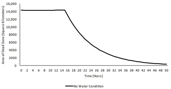
Figure 6.
No Water model results. The graph depicts the initial area of the dead zone changing across time under the synthetic scenario where no water flows through the basin, all other variables remaining constant.
Extreme conditions tests were not intended to reflect real-life events but to simulate logical behavior outside known boundaries of inputs based on the existing knowledge about the system. The model structure allows nitrogen to be delivered to the Gulf and contribute to the dead zone as long as sufficient water flows through the system. Initially, water is supplied from the water stocks, but when precipitation is deactivated for the test, the stocks eventually become depleted. Consequently, the area of the dead zone gradually shrinks due to de-nitrification, as no additional nitrogen is added. Once the water runs out, nitrification ceases because there are no means for nitrogen to be transported to the Northern Gulf of Mexico. This scenario is represented in the model by the Lower MARB Dead Pool Storage variable, which halts water discharge when the inflow is less than 500 million cubic meters due to insufficient elevation.
In the second extreme conditions test, we simulated the opposite scenario through the Permanent Severe Flood Condition test. The scenario was set by tripling the precipitation inputs and halving the conveyance time to represent the flooding scenario. The result was a temporary sharp increase in the area of the dead zone during the first two years. At the end of the 50 years, the model exhibited a consistently lower resulting area of dead zone that closely resembled the average shown in the base case run (Figure 7). This increase was due to the rapid initial transportation of the existing nitrogen load into the Northern Gulf of Mexico, which, combined with the additional annual load of nitrogen, contributed to the sharp increase in dead zone area. It can be inferred from this simulation run that the model allows the additional water to increase the area of the dead zone consistently in the long term only if additional nitrogen is available for transport.
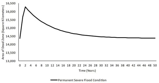
Figure 7.
Permanent Severe Flood Condition model results. The graph depicts the initial area of the dead zone changing across time under the synthetic scenario where an excessive amount of water flows through the basin in comparison to the base model. All other variables, including nitrogen load, remain constant.
3.3. Sensitivity Test Results
For the sensitivity test simulation, we assessed the model’s response to varying nitrogen concentration inputs and volume of flow inputs. A total of five (5) simulations were conducted: one with reduced nitrogen input (Figure 8), another with increased nitrogen input (Figure 9), and three (3) combinations of these two inputs with different levels of water volume. These simulations were compared to each other, as well as to the base model run. A fundamental goal of conducting this series of tests was to uncover the weight of each of the two key inputs of the system (nitrogen and water) and whether combinations of changes in these would incur changes distinct from those occurring independently.
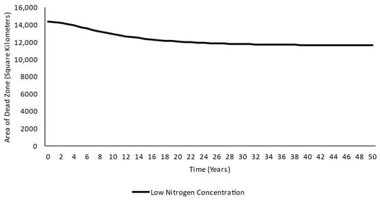
Figure 8.
Low nitrogen input model results. The graph depicts the initial area of the dead zone changing across time under the synthetic scenario where nitrogen discharge from the basin is permanently reduced in comparison to the base model, with all other variables remaining constant.
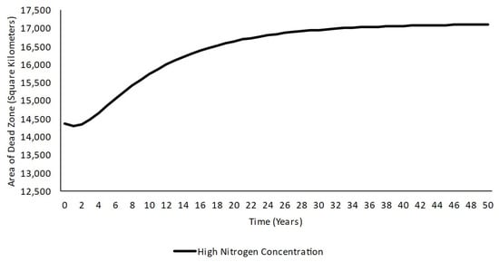
Figure 9.
High nitrogen input model results. The graph depicts the initial area of the dead zone changing across time under the synthetic scenario where nitrogen discharge from the basin is permanently increased in comparison to the base model, with all other variables remaining constant.
The first sensitivity test assessed the area of the dead zone with a low nitrogen input (Figure 8). The scenario was achieved by removing 10,000.000 kg of nitrogen from each of the two sources in the model. The resulting behavior was that the dead zone area initially decreased its size steadily. The reduction rate eventually began to slow down and eventually leveled off within the first ten years. The result was a reduction of ~2700 square kilometers from the dead zone compared to the base run scenario.
In the second sensitivity test, the response to a high nitrogen input was assessed (Figure 9). The scenario was achieved by adding 10,000.000 kg of nitrogen from each of the two sources in the model. The behavior exhibited was a smooth increase in the dead zone area starting in year two. The area of the dead zone eventually leveled off near year 50 after exhibiting growth followed by transition to equilibrium (i.e., increased at a decreasing rate). Holding other factors constant, higher nitrogen input led to a significantly larger dead zone, amounting to a change in similar proportion to the low nitrogen test (~2700 square kilometers), this time representing an increase compared to the base case. These results confirm the model’s consistency when inputs were deliberately modified in either direction.
To evaluate the weight of nitrogen inputs in the area of the dead zone compared to the effect of the volume of flow in the MARB, a combination of two sensitivity adjustments was used for three additional simulation runs. A low nitrogen and low runoff scenario were achieved via reduced precipitation variables to the tune of 25%, combined with the same reduction of nitrogen as the Low Nitrogen Concentration test. The result was virtually identical to the other two tests, but a sharp decrease in the area dead zone was observed during the first 10 years, momentarily exceeding the net decrease seen by year 50 (Figure 10).
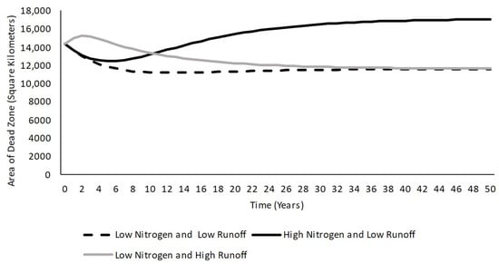
Figure 10.
Low nitrogen and low runoff/high nitrogen and low runoff/low nitrogen and high runoff results. Different combinations of simultaneous inputs were used to test the sensitivity of the model. For runoff conditions (high or low), water inputs were modified ±25%. Nitrogen inputs were modified in the same ways as the previous high/low nitrogen scenarios (±10,000,000 kg).
Combining the high nitrogen setup with the previously described reduced runoff created other distinct results. The shape of the resulting graph was similar to that of the High Nitrogen Condition trial. However, the reduced runoff had the effect of delaying the increase in the dead zone (Figure 10). For example, by year 10, the area of the dead zone in this scenario was ~2552 square kilometers smaller than the one yielded when nitrogen was the only input modified. By the end of the 50 years, the area was still marginally smaller by ~56.
The final combination for the sensitivity testing was low nitrogen paired with high runoff. The result after 50 years is almost identical as the area yielded by the Low Nitrogen Condition scenario is only ~6 square kilometers greater. The greatest distinction could be observed in the first three years, where the area of the dead zone in this scenario momentarily increases. This behavior can be explained by the increased water that has initially overwhelmed (carrying additional nitrogen existing in the model since time step 0) the capacity of the Gulf to remove hypoxia naturally. The area of the dead zone eventually decreased as no additional nitrogen was inputted, leading to the almost identical decline experienced by the simpler version of the sensitivity test. As expected, the combination that yielded the smallest area of dead zone was the low nitrogen and low runoff pairing.
3.4. Management Decisions and Policy Analyses Test Results
For the policy test simulations, the model was configured to evaluate the impact of implementing control policies aimed at reducing nitrogen and water inputs by 20% compared to the base model’s nitrogen inputs, mimicking real-world environmental goals. The control policy’s effects were evaluated without a starting dead zone area to evaluate the behavior of the system when a response is conditioned for a specific threshold and the effect of the timeliness of said response. The policy scenarios were put together by adding a new variable that would receive feedback from the dead zone surface area variable and would exert an effect on nitrogen, water, or both, once a specific threshold of area of dead zone was surpassed. Here, we use a threshold value set at 12,949.94 square kilometers. This figure resembles the average hypoxic area we have observed in the real world in recent years and has prompted multiple organizations to devise strategies to address the issue. Upon activation, the control policy resulted in a cumulative twenty percent reduction in MARB nitrogen inputs, water, or both, leading to changes in the area of the dead zone at different points of the simulation depending on the policy tested (Figure 11).
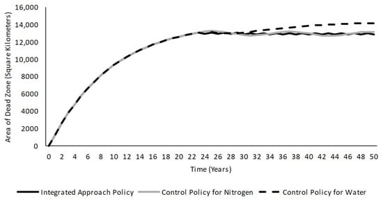
Figure 11.
Control policy vs. no control policy results. The no control policy (black) represents the simulation output given the conditions of the base model without intervention. The control policy (grey) shows the impact of a restrictive policy that controls the transport of nitrogen after a specific threshold of hypoxic area is surpassed.
The first policy test evaluates the reduction of nitrogen by 20%, reflecting Hypoxia Task Force objectives. Achieving such a goal is realistic when taking on certain tradeoffs. A reduction in nitrogen can be achieved through various means. For example, caps or taxes on fertilizer use, runoff mitigation, or potential price increases in raw materials used in synthetic fertilizers. The model represented these possibilities using a switch equation embedded in an auxiliary variable named “policy switch”. As mentioned previously, it was connected to all nitrogen input inflows. This switch acts as a multiplier in equations estimating nitrogen transport before it enters any stock. It remains off unless the dead zone area exceeds 12,949.94 square kilometers, at which point the multiplier (0.80) is applied to every nitrogen source via the IF THEN ELSE function. The multiplication then represents a 20% decrease in the original nitrogen inputs. The result was a containment of the dead zone within an area near the threshold value.
The second and third policy tests evaluated a similar response but reducing runoff and a combination of nitrogen and runoff, respectively. The same policy switch variable and equation were used, the only difference being the variables it was connected to (water, nitrogen-related, or both). The result of the water control policy was a greater dead zone area compared to the ones produced by the other two policies. The trajectory of the graph also indicated that the area of the dead zone was still increasing by year 50, hinting that it would eventually reach over 14,000 square kilometers. The Integrated Approach Policy proved to be the most effective, producing an area of dead zone ~1507 square kilometers smaller than in the base run and ~292 square kilometers smaller than the second-best policy (Control Policy for Nitrogen). The Integrated Approach Policy and the Control Policy for Nitrogen effectively inhibited the area of the dead zone from reaching the predetermined level it should have obtained given the default state of the system, while the Control Policy for Water only delayed the expansion of the dead zone.
3.5. Overall Results
The overall outcome reveals that focusing on specific control efforts, such as reducing nitrogen or runoff, is effective to an extent limited by their respective conditioning factors within the system. The model’s behavior under varying nutrient and water inputs, including extreme scenarios, offers insights into the extent of the effectiveness of different approaches, including combining them. For instance, nutrient suppression can have a significant impact in the long term while other variables remain constant, but its benefits can be negated by increased runoff in the short run, making the approach seem ineffective at first glance and more likely to be abandoned. Conversely, runoff suppression within realistic levels may initially reduce the dead zone area, but this positive effect may be eventually reversed in the case that the annual nutrient loads remain the same or increase. The extreme scenario simulations illustrated hypothetical situations where the dead zone could be significantly reduced or eliminated, serving as references for the system’s behavior when pushed to its limits and illustrating possible results from parameters not conceived in the real world yet. Results from the SD model suggest that an integrated strategy is needed to maximize the effectiveness of efforts to control and reduce the area of the dead zone. Policy tests specifically underscore the importance of the timeliness of reaction; the approach was successful at halting the dead zone expansion but would have been more effective had the threshold been set at a lower level and activated the policy at an earlier time.
4. Discussion
The SD approach used to assess the formation of the dead zone in the Gulf of Mexico has already been employed in other studies seeking to understand environmental management issues and the effect of different interventions via simulations using Vensim. For example, Collins et al. used an SD model to explore how interactions between physical and political systems in forest fire management interact to influence the effect of different policies that implicate the allocation of resources to fire suppression or fire prevention in the forests of Portugal [20]. However, no prior work has been published where SD was used to study the dead zone of the Gulf, to the best of our knowledge.
The insights from the various simulations stemming from the model highlight how devising interventions for controlling the area of the dead zone is challenging due to the scale of the MARB and the extent of time that must pass for results to be visible. Model results underscored the benefits of balanced, integrated approaches when discussing the suppression of nitrogen and runoff along the basin. The timeliness of interventions also proved to be crucial in policy tests which, while effective, would have been of higher leverage if used when the dead zone was still smaller in this specific set of simulations. Among the ‘feasible’ scenarios, the dead zone could be reduced and have its size contained, but limited to reaching desired environmental goals.
Based on model results, barring the extreme scenario tests, neither reduced nitrogen nor runoff from major watersheds achieve the known official goal of reducing the dead zone to less than 5000 square kilometers by 2025. However, it can be inferred from the model that reduction of nitrogen and runoff may still allow a substantial reduction of the dead zone compared to recent levels, namely that seen during its peak in 2017. Model results suggest that other factors that influence the formation of the dead zone should be studied beyond nitrogen, which was the isolated variable that was observed in this case. Based on model behaviors, more violent reductions exclusively on the inputs examined could reduce the dead zone to desired levels. However, the feasibility of said reductions may be constrained to economic and social tradeoffs, as well as technical limitations.
When planning potential interventions, it is crucial to consider the nearly unchangeable constraints of the MARB that were highlighted in the model used in this study. Synthetic nitrogen sources are vital for modern food production and security [21]. Efforts to reduce the dead zone should not compromise essential agricultural production. The Midwest, which encompasses most of the MARB, is a highly productive agricultural region, producing 65% of the United States’ corn and soybeans. Interventions must strike a balance to achieve net gains between fisheries, tourism, and recreation in the Gulf of Mexico, as well as food and economic security in the Midwest.
Fortunately, incentives to seek solutions of this nature do exist. Over half of the streams in the United States are negatively impacted in terms of water quality due to the increasing usage of fertilizer [22]. The Midwest particularly faces the issue of frequent flooding as a result of excessive precipitation and sometimes snowmelt [23] that further aggravate the leaching of nutrients with the soil having a limited capacity for retention. Integrated approaches, such as nutrient management, are examples of methods where progress can be attained in both nutrient and runoff reduction. Nutrient management can be described as “the science and art directed to link soil, crop, weather, and hydrologic factors with cultural, irrigation, and soil and water conservation practices to achieve the goals of optimizing nutrient use efficiency, yields, crop quality, and economic returns, while reducing off-site transport of nutrients” [24]. Buffer strips, nutrient recycling, and irrigation management are some examples of practices that can be part of a nutrient management-based strategy
The model’s causal relationships align with existing literature and insights from professionals monitoring the Gulf’s dead zone. It is important to recognize that SD models do not provide statistically precise estimates, with typical accuracy seldom exceeding 40% [25]. These models illustrate the proportion and direction of outcomes resulting from observable processes within a system. They also serve as a tool to evaluate the impact of managerial decisions across multiple interconnected areas. While the visual representations in the model display specific numerical scales, these figures should not be taken as exact values. Instead, the numerical outputs were meant to explain and test the directional relationships between variables. Engaging with experts and conducting fieldwork that integrates into a Vensim SD model could enhance the accuracy and predictive value of the data.
Although SD is a valuable tool for understanding complex system behaviors, it has limitations due to its reliance on deterministic causal processes. Real-world systems, particularly in environmental management, are influenced by significant uncertainties, primarily stemming from human interventions. These interventions continuously interact with systems to alter their trajectories. As a result, a deterministic simulation model, which depends on fixed relationships among political, social, and physical factors, cannot fully capture the evolving dynamics of a system influenced by numerous unaccounted-for factors. This inherent limitation underscores the importance of considering uncertainties and external variables when using SD models for policy and decision-making in environmental management.
This study does not consider the economic implications of runoff suppression, nitrogen suppression, and marine life loss from the dead zone. While the policies defined might reduce the parameters leading to dead zone creation, pursuing this objective might conflict with broader system goals, such as agricultural economic stability and urban development demands. This paper does not incorporate incentives resulting from the system’s economic state and its stakeholders. The perceived success of a strategy in real life may depend not only on restoring or conserving ecosystem services but also on the economic returns they generate. Future research on the MARB could develop a model that includes socio-economic factors alongside the environmental system already modeled in this paper. One of SD’s strengths is its ability to expand model boundaries to incorporate other subsystems. However, expanding the system’s scope must be carefully balanced against the potential loss of specificity in individual components.
5. Conclusions
The sensitivity and policy tests allowed us to draw several key inferences. It is clear that exclusively reducing nitrogen, whether through regulations, practice adoption, or technological advancement, does reduce the area of the dead zone substantially. However, the effect is insufficient to reduce it to the desired levels soon, specifically to the less than 5000 square kilometers that is the goal of the EPA Hypoxia Task Force. Policies tested in this study tend to halt further expansion or minimize growth relative to the average but do not reverse the accumulation of hypoxic square kilometers throughout the simulation enough to get to the desired levels. Similarly, reducing the water flow from the basin alone only delays the inevitable transport of pollution into the Gulf if the discharge of nitrogen is unchanged. This change delays the peak dead zone area but does not prevent the dead zone from expanding if nitrogen levels are the same or higher. A reduction in the volume of flow is one of the few scenarios that would stop dead zone formation altogether. This scenario is highly unlikely in the real-life MARB system. The model also showed that a hypothetical total absence of water or an unrealistically low nitrogen concentration would reduce the dead zone.
This model offers new insights into the phenomenon of hypoxic area formation. The SD approach was used to devise a method to quantify the causes and effects among stocks and variables of different inputs (nitrogen and water). The approach could translate the interaction of variables and use them to estimate the area of the dead zone across extended periods. We were able to recreate realistic behavior in a model focusing on nitrogen and water as the system’s main drivers. This approach made way for a variety of scenarios to be adapted to the model to gain feedback on the potential effects of real-world interventions. Our observations from simulated scenarios indicate that the area of the dead zone can be reduced and controlled under specific limitations. Additionally, the model set a foundation that can be expanded upon to incorporate other contributing elements to the dead zone, such as other nutrients or economic influences or interactions.
Author Contributions
Conceptualization, L.M.-V., J.L. and K.G.; methodology, L.M.-V., J.L. and K.G.; software, L.M.-V., J.L. and K.G.; validation, L.M.-V.; formal analysis, L.M.-V., J.L. and K.G.; investigation, L.M.-V., J.L. and K.G.; resources, B.T. and A.A.; data curation, L.M.-V.; writing—original draft preparation, L.M.-V., J.L. and K.G.; writing—review and editing, L.M.-V., B.T. and A.A.; visualization, L.M.-V.; supervision, L.M.-V.; project administration, L.M.-V.; funding acquisition, B.T. and A.A. All authors have read and agreed to the published version of the manuscript.
Funding
This work was partially supported by United States Department of Agriculture’s Research and Extension Experiences for Undergraduates Grant No. 2020-67037-30652 and the National Science Foundation’s Center for Research Excellence in Science and Technology (CREST) Award No. 1914745.
Data Availability Statement
Data is contained within the article.
Conflicts of Interest
The authors declare no conflicts of interest.
Appendix A
Table A1.
Table of equations. Note that the variables Lower MARB Dead Pool Storage and policy switch variables, including their presence on equations, were included only in the no water condition and control policy implementation condition tests, respectively. The mention of these variables is marked with an asterisk (*) on the table of equations. Inputs that change for specific tests are also specified on the Equation column.
| Variable | Type | Equation | Units |
|---|---|---|---|
| Arkansas River | Flow | Default: Arkansas River precip Depth*Arkansas River Surface Policy test (water and integrated) equation: (Arkansas River precip Depth*Arkansas River Surface)*Policy Switch | m*m*m/Year |
| Arkansas River Precip Depth | Auxiliary variable | Default: 0.5 Permanent Severe Flood Condition test equation: 1.5 No Water Condition test equation: 0 Sensitivity Low Water tests equation: 0.25 Sensitivity High Water tests equation: 0.75 | m/Year |
| Arkansas River Surface | Auxiliary variable | 2.12 × 10¹¹ | m*m |
| Conveyance Time in Lower MARB | Auxiliary variable | 0.5 Permanent Severe Flood Condition test equation: 1 Sensitivity Low Water tests equation: 0.25 Sensitivity High Water tests equation: 0.75 | Dmnl/Year |
| Conveyance Time in Upper MARB | Auxiliary variable | Permanent Severe Flood Condition test equation: 1 Sensitivity Low Water tests equation: 0.25 Sensitivity High Water tests equation: 0.75 | Dmnl/Year |
| Dead Zone Expansion Factor | Auxiliary variable | 1.47364 × 10⁻⁵ | Square Kilometers/Kilograms |
| Dead Zone Surface Area | Stock | INTEG (Surface Area Gained-Surface Area Lost, Initial Area of dead zone) | Square Kilometers |
| De-nitrification Rate | Auxiliary variable | 0.1 | Dmnl/Year |
| FINAL TIME | Model setting | 50 | Year |
| Headwater MARB Inflow | Inflow | Headwater MARB Volume of flow | m*m*m/Year |
| Headwater MARB Precipitation Depth | Auxiliary variable | Default: 0.5 Permanent Severe Flood Condition test equation: 1.5 No Water Condition test equation: 0 | m/Year |
| Headwater MARB Surface Area | Auxiliary variable | 2.12 × 10¹¹ | m*m |
| Headwater MARB Volume of flow | Auxiliary variable | Default: Headwater MARB Precipitation depth*Headwater MARB Surface area Policy test (water and integrated) equation: (Headwater MARB Precipitation depth*Headwater MARB Surface area)*Policy Switch | m*m*m/Year |
| Initial Area of dead zone | Auxiliary variable | Default equation; 14,370.549 Policy tests (any) equation: 0 | Square Kilometers |
| Initial Lower MARB Nitrogen | Auxiliary variable | 198,317,000 | Kilograms |
| Initial Lower MARB Water | Auxiliary variable | 1.375 × 10¹² | m*m*m |
| Initial N Load Upper MARB | Auxiliary variable | Default: 52,159,400 Policy test (nitrogen and integrated) equation: 52,159,400*Policy Switch Sensitivity High Nitrogen tests equation: 62,159,400 Sensitivity Low Nitrogen tests equation: 42,159,400 | Kilograms/Year |
| Initial N Load Lower MARB | Auxiliary variable | Default: 52,159,400 Policy test (nitrogen and integrated) equation: 52,159,400*Policy Switch Sensitivity High Nitrogen tests equation: 62,159,400 Sensitivity Low Nitrogen tests equation: 42,159,400 | Kilograms/Year |
| Initial Time | Model setting | 0 | Year |
| Initial Upper MARB Nitrogen | Auxiliary variable | 107,091,000 | Kilograms |
| Initial Upper MARB Water | Auxiliary variable | 6.125 × 10¹¹ | m*m*m |
| Lower MARB | Stock | INTEG (Arkansas River+Red River Water Inflow+Upper MARB outflow-Lower MARB Outflow, Initial Lower MARB Water) | m*m*m |
| * Lower MARB Dead Pool Storage | Auxilary Variable | 5 × 10⁸ | m*m*m |
| Lower MARB N | Stock | INTEG (Lower MARB N Inflow+Transported MARB N-Lower MARB N Outflow, Initial Lower MARB Nitrogen) | Kilograms |
| Lower MARB N Inflow | Flow | Initial N Load in Lower MARB | Kilograms/Year |
| Lower MARB N Outflow | Flow | Lower MARB Outflow*N concentration in Lower MARB | Kilograms/Year |
| Lower MARB Outflow | Flow | Default equation: Lower MARB*Conveyance Time in Lower MARB No Water Condition test equation: IF THEN ELSE(Lower MARB>Lower MARB Dead Pool Storage, Lower MARB*Conveyence time in Lower MARB, 0) Policy test (water and integrated) equation: (Lower MARB*Conveyance Time in Lower MARB)*Policy Switch | m*m*m/Year |
| Maximum Area that can cease to be hypoxic in 1 year | Auxiliary variable | 1000 | Square kilometers/Year |
| Missouri River Inflow | Flow | Default: Missouri River Surface*Missouri River Precip Depth Policy test (water and integrated) equation: (Missouri River Surface*Missouri River Precip Depth)*Policy Switch | m*m*m/Year |
| Missouri River Precip Depth | Auxiliary variable | Default: 0.5 Permanent Severe Flood Condition test equation: 1.5 No Water Condition test equation: 0 Sensitivity Low Water tests equation: 0.25 Sensitivity High Water tests equation: 0.75 | m/Year |
| Missouri River Surface | Auxiliary variable | 2.12 × 10¹¹ | Square meters |
| N Concentration in Lower MARB | Auxiliary variable | Lower MARB N/Lower MARB | Kilograms/m*m*m |
| N Concentration in Upper MARB | Auxiliary variable | Upper MARB N/Upper MARB | Kilograms/m*m*m |
| Ohio River Inflow | Flow | Default: Ohio River Surface*Ohio River Precip Depth Policy test (water and integrated) equation: (Ohio River Surface*Ohio River Precip Depth)*Policy Switch | m*m*m/Year |
| Ohio River Precip Depth | Auxiliary variable | Deafult: 0.5 Permanent Severe Flood Condition test equation: 1.5 No Water Condition test equation: 0 Sensitivity Low Water tests equation: 0.25 Sensitivity High Water tests equation: 0.75 | m/Year |
| Ohio River Surface | Auxiliary variable | 2.12 × 10¹¹ | Square meters |
| * Policy switch | Auxilary variable | Default: Variable Absent Policy Test (any) Equation: IF THEN ELSE(Dead Zone Surface Area > 12,949.94, 0.8, 1) | dmnl |
| Red River Precip Depth | Auxiliary variable | Default: 0.5 Permanent Severe Flood Condition test equation: 1.5 No Water Condition test equation: 0 Sensitivity Low Water tests equation: 0.25 Sensitivity High Water tests equation: 0.75 | m/Year |
| Red River Surface | Auxiliary variable | 2.12 × 10¹¹ | Square meters |
| Red River Water Inflow | Flow | Default: Red River Precip Depth*Red River Surface Policy test (water and integrated) equation: (Red River Precip Depth*Red River Surface)*Policy Switch | m*m*m/Year |
| Saveper | Model setting | Time Step | Year |
| Surface Area Gained | Flow | Lower MARB N Outflow*Dead Zone expansion factor | Square Kilometers/Year |
| Surface Area Lost | Flow | MIN ((“Dead Zone (Surface Area)”*De-nitrification Rate), Maximum Area that can cease to be hypoxic in 1 year) | Square Kilometers/Year |
| Time Step | Model setting | 1 | Year |
| Transported MARB N | Flow | Upper MARB outflow*N concentration in upper MARB | Kilograms/Year |
| Upper MARB | Stock | INTEG (Headwater MARB Inflow+Missouri River Inflow+Ohio River Inflow-Upper MARB outflow, Initial Upper MARB water) | m*m*m |
| Upper MARB N | Stock | INTEG (Upper MARB Nitrogen Inflow-Transported MARB N, Initial Upper MARB Nitrogen) | Kilograms |
| Upper MARB Nitrogen Inflow | Flow | Initial N Load from Upper MARB | Kilograms/Year |
| Upper MARB outflow | Flow | Default: Upper MARB*Conveyance Time in Upper MARB Policy test (water and integrated) equation:(Upper MARB*Conveyance Time in Upper MARB)*Policy Switch | m*m*m/Year |
References
- US Department of Commerce, National Oceanic and Atmospheric Administration. What Is a Dead Zone? NOAA’s National Ocean Service, 14 March 2019. Available online: https://oceanservice.noaa.gov/facts/deadzone.html (accessed on 1 February 2023).
- Le Moal, M.; Gascuel-Odoux, C.; Ménesguen, A.; Souchon, Y.; Étrillard, C.; Levain, A.; Moatar, F.; Pannard, A.; Souchu, P.; Lefebvre, A.; et al. Eutrophication: A New Wine in an Old Bottle? Sci. Total Environ. 2019, 651, 1–11. [Google Scholar] [CrossRef] [PubMed]
- Schindler, D.; Vallentyne, J. Algal Bowl: Overfertilization of the World’s Freshwaters and Estuaries; Earthscan: London, UK, 2008; ISBN 9781844076239. [Google Scholar]
- Diaz, R.; Rosenberg, R. Spreading Dead Zones and Consequences for Marine Ecosystems. Science 2008, 321, 926–929. [Google Scholar] [CrossRef] [PubMed]
- Environmental Protection Agency. Major River Systems within the Mississippi River Basin.Svg. Wikimedia Commons. 2023. Available online: https://commons.wikimedia.org/wiki/File:Major_River_Systems_within_the_Mississippi_River_Basin.svg (accessed on 1 February 2023).
- Bianchi, T.S.; DiMarco, S.; Cowan, J.; Hetland, R.; Chapman, P.; Day, J.; Allison, M. The Science of Hypoxia in the Northern Gulf of Mexico: A Review. Sci. Total Environ. 2010, 408, 1471–1484. [Google Scholar] [CrossRef] [PubMed]
- NASA Earth Observatory. Public Domain. Aquatic Dead Zones. Wikimedia Commons. 2010. Available online: https://commons.wikimedia.org/wiki/File:Aquatic_Dead_Zones.jpg (accessed on 1 February 2023).
- Sterman, J.D. Business Dynamics: Systems Thinking and Modeling for a Complex World; Irwin McGraw-Hill: Boston, MA, USA, 2000. [Google Scholar]
- Turner, B.L.; Menendez, H.M., III; Gates, R.; Tedeschi, L.O.; Atzori, A.S. System dynamics modeling for agricultural and natural resource management issues: Review of some past cases and forecasting future roles. Resources 2016, 5, 40. [Google Scholar] [CrossRef]
- Ford, A. Modeling the Environment; Island Press: Washington, DC, USA, 2009. [Google Scholar]
- Turner, B.L. Model laboratories: A quick-start guide for design of simulation experiments for dynamic systems models. Ecol. Model. 2020, 434, 109246. [Google Scholar] [CrossRef]
- NOAA. Map of Measured Gulf Hypoxia Zone. Wikimedia Commons. 2021. Available online: https://commons.wikimedia.org/wiki/File:IMAGE-Map_of_measured_Gulf_hypoxia_zone,_July_25-31,_2021-LUMCON-NOAA.png (accessed on 1 February 2023).
- Braun, W. System Archetypes. The Systems Modeling Workbook. 2002. Available online: https://www.albany.edu/faculty/gpr/PAD724/724WebArticles/sys_archetypes.pdf (accessed on 1 August 2024).
- Marandure, T.; Dzama, K.; Bennett, J.; Makombe, G.; Mapiye, C. Application of System Dynamics Modelling in Evaluating Sustainability of Low-Input Ruminant Farming Systems in Eastern Cape Province, South Africa. Ecol. Model. 2020, 438, 109294. [Google Scholar] [CrossRef]
- Guemouria, A.; Chehbouni, A.; Belaqziz, S.; Epule Epule, T.; Ait Brahim, Y.; El Khalki, E.; Dhiba, D.; Bouchaou, L. System dynamics approach for water resources management: A case study from the souss-massa basin. Water 2023, 15, 1506. [Google Scholar] [CrossRef]
- Jordan, E. As Conservation Lags, So Does Progress in Slashing Gulf’s ‘Dead Zone’ Republican Eagle. 2024. Available online: https://www.republicaneagle.com/news/as-conservation-lags-so-does-progress-in-slashing-gulfs-dead-zone/article_bb12c078-3997-11ef-b659-e7197466af7d.html (accessed on 1 July 2024).
- Forrester, J.W.; Senge, P. Tests for building confidence in system dynamics models. In System Dynamics; Legasto, A.J., Forrester, J.W., Lyneis, J., Eds.; TIMS Studies in the Management Sciences 14; North-Holland: New York, NY, USA, 1980; pp. 209–228. [Google Scholar]
- Schaetzl, R.; Severin, G.T.; Muller, R.; Kesel, R.; Wallenfeldt, J. Mississippi River. Encyclopedia Britannica. 2024. Available online: https://www.britannica.com/place/Mississippi-River (accessed on 1 February 2023).
- Rabalais, N.; Turner, E.; Wiseman, W. Hypoxia in the Gulf of Mexico. J. Environ. Qual. 2001, 30, 320–329. [Google Scholar] [CrossRef] [PubMed]
- Collins, R.; de Neufville, R.; Claro, J.; Oliveira, T.; Pacheco, A. Forest Fire Management to Avoid Unintended Consequences: A Case Study of Portugal Using System Dynamics. J. Environ. Manag. 2013, 130, 1–9. [Google Scholar] [CrossRef] [PubMed]
- Ehrlich, P.; Ehrlich, A.; Daily, G. Food Security, Population and Environment. Popul. Dev. Rev. 1993, 19, 1–32. [Google Scholar] [CrossRef]
- Environmental Protection Agency. Hypoxia in the northern Gulf of Mexico. In EPA Mississippi River/Gulf of Mexico Hypoxia Task Force. 2007. Available online: https://www.epa.gov/sites/default/files/2015-03/documents/2008_1_31_msbasin_sab_report_2007.pdf (accessed on 1 February 2023).
- Pryor, S.; Scavia, D.; Downer, C.; Gaden, M.; Iverson, L.; Nordstrom, R.; Patz, J.; Robertson, G. Ch. 18: Midwest. Climate Change Impacts in the United States: The Third National Climate Assessment; U.S. Global Change Research Program (USGCRP): Washington, DC, USA, 2014. [CrossRef]
- Delgado, J.; Lemunyon, J. Nutrient management. In Encyclopedia of Soil Science; Marcel Decker: New York, NY, USA, 2006; pp. 1157–1160. [Google Scholar]
- Chahal, K.; Eldabi, T. A multi-perspective comparison for selection between system dynamics and discrete event simulation. Int. J. Bus. Inf. Syst. 2010, 6, 4. [Google Scholar] [CrossRef]
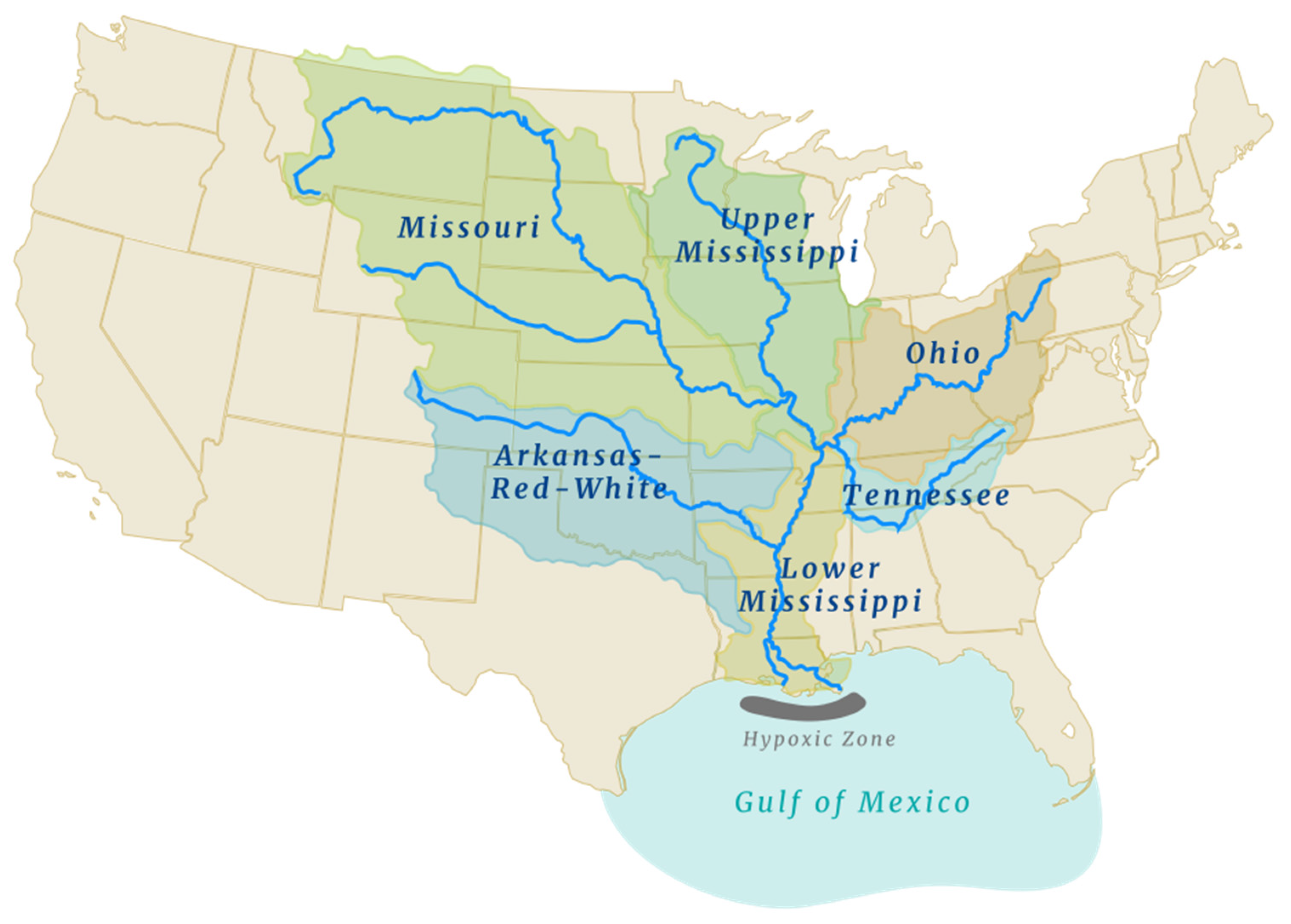

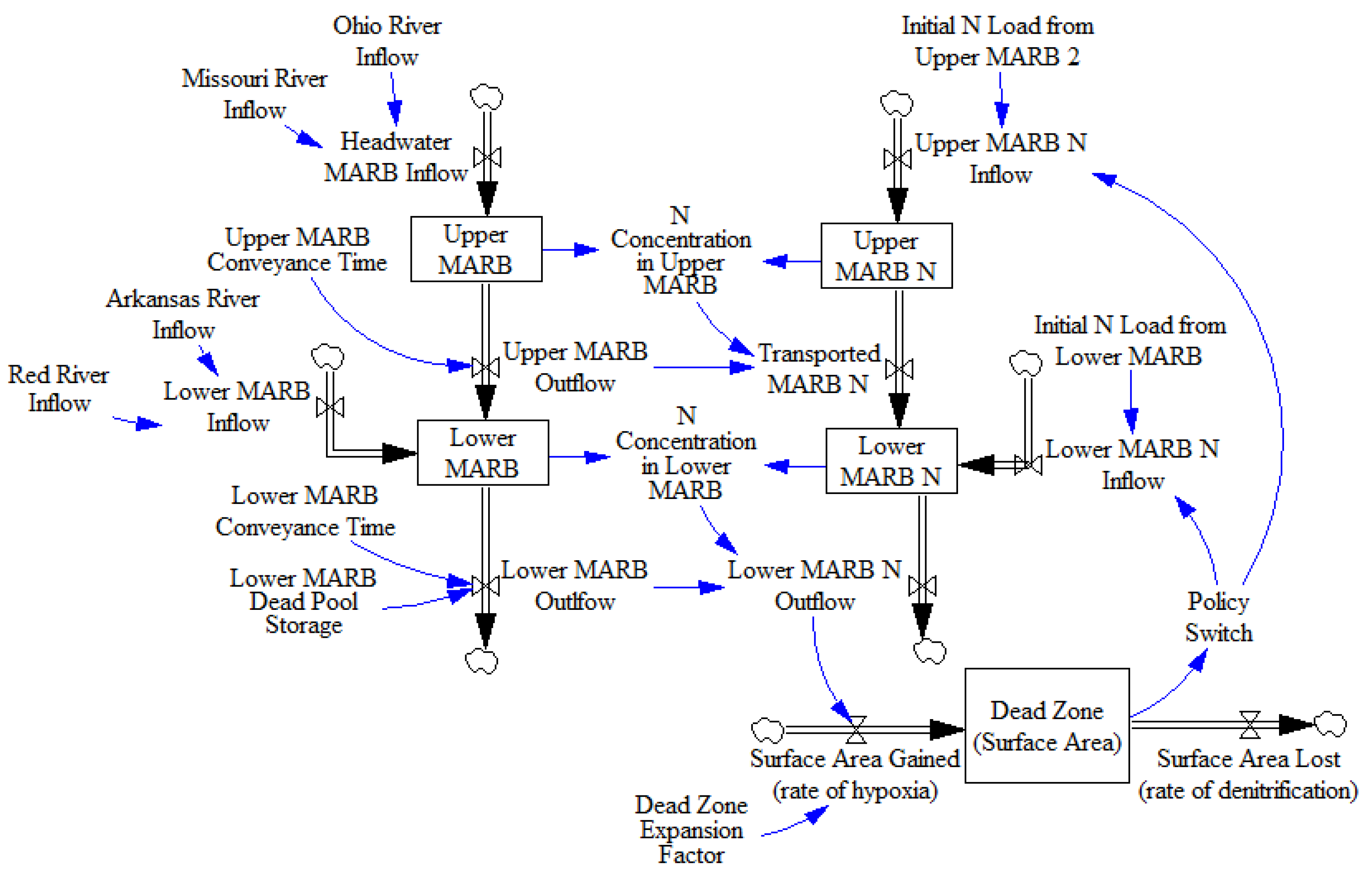
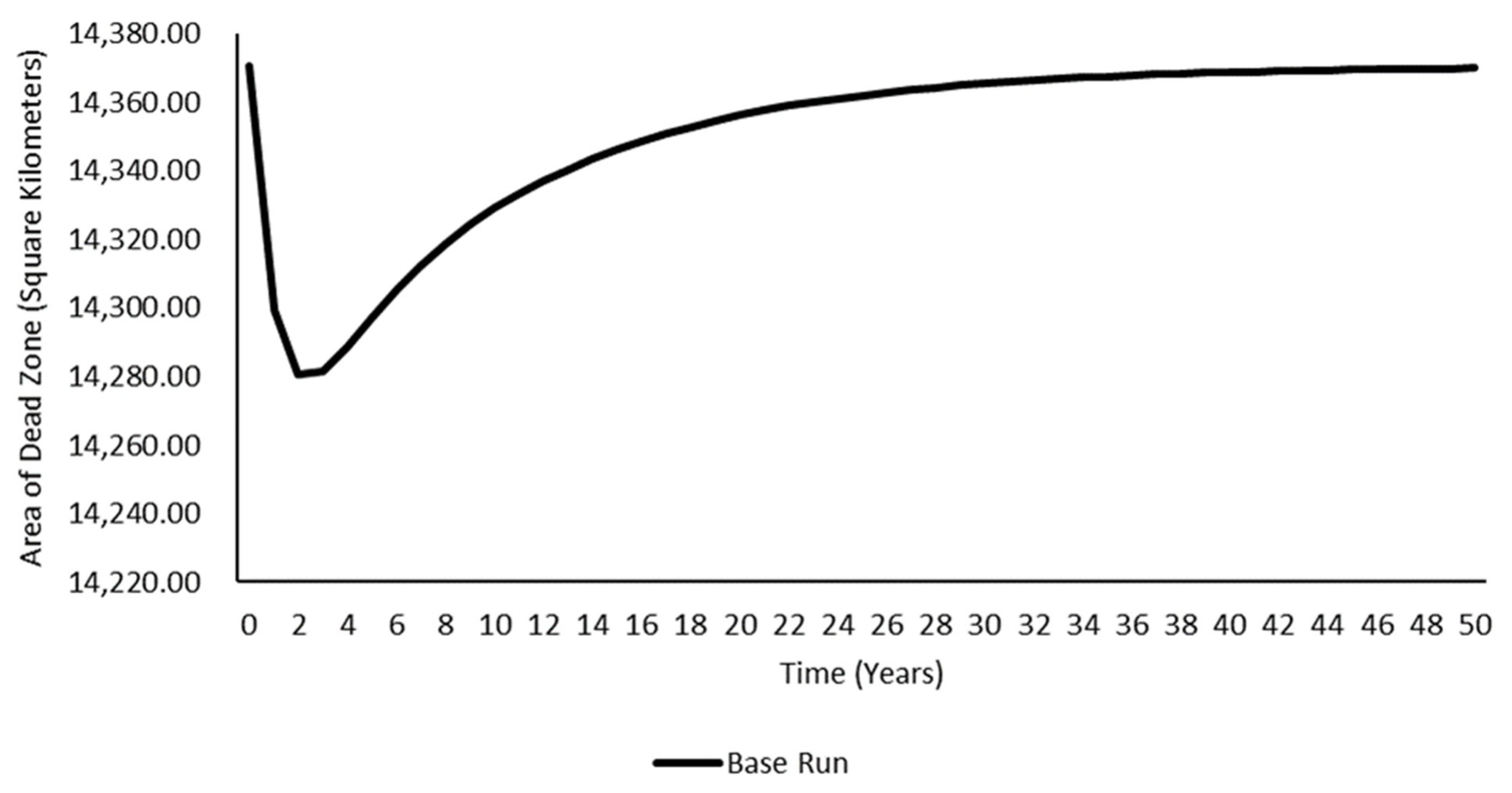
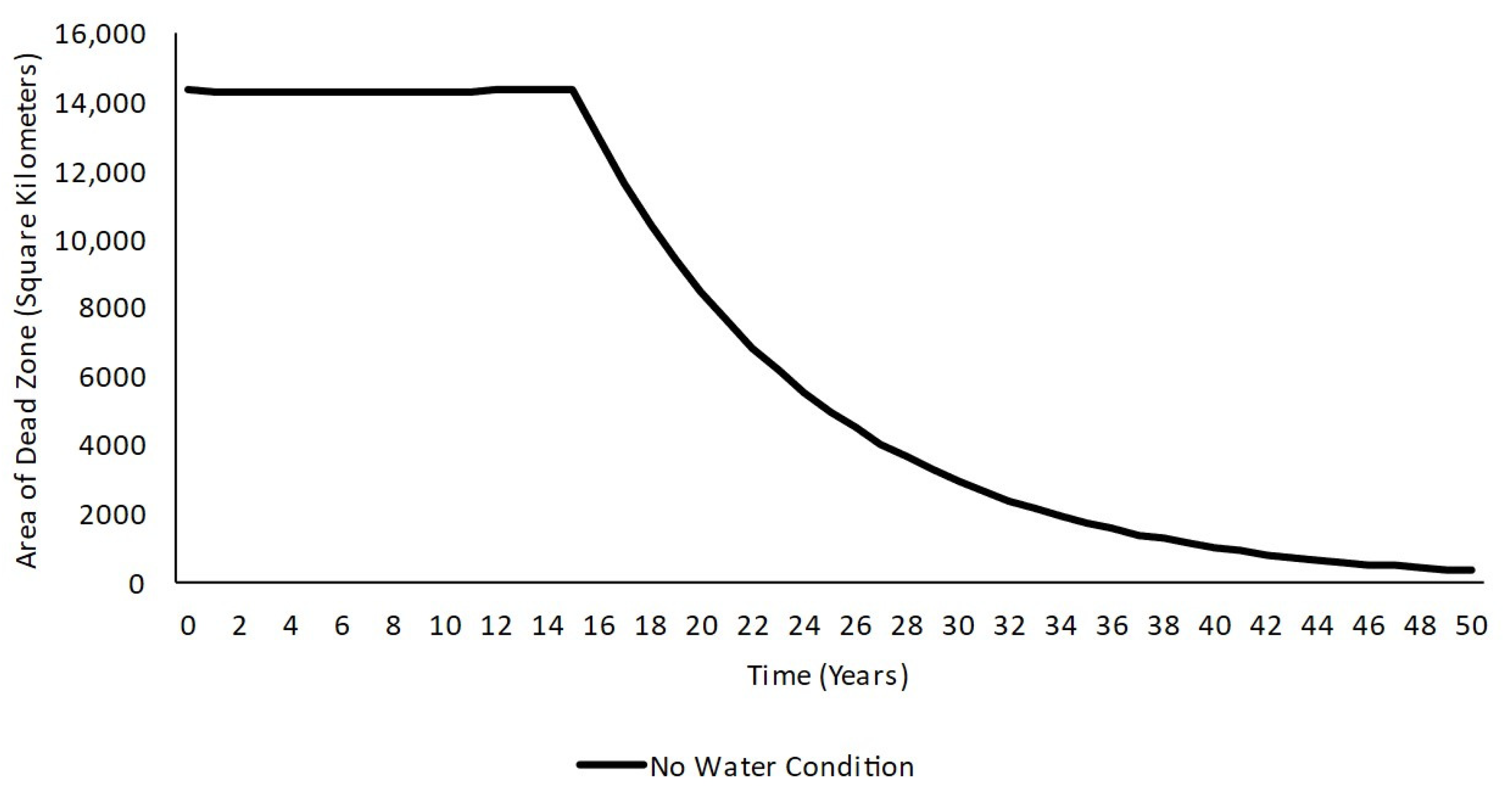
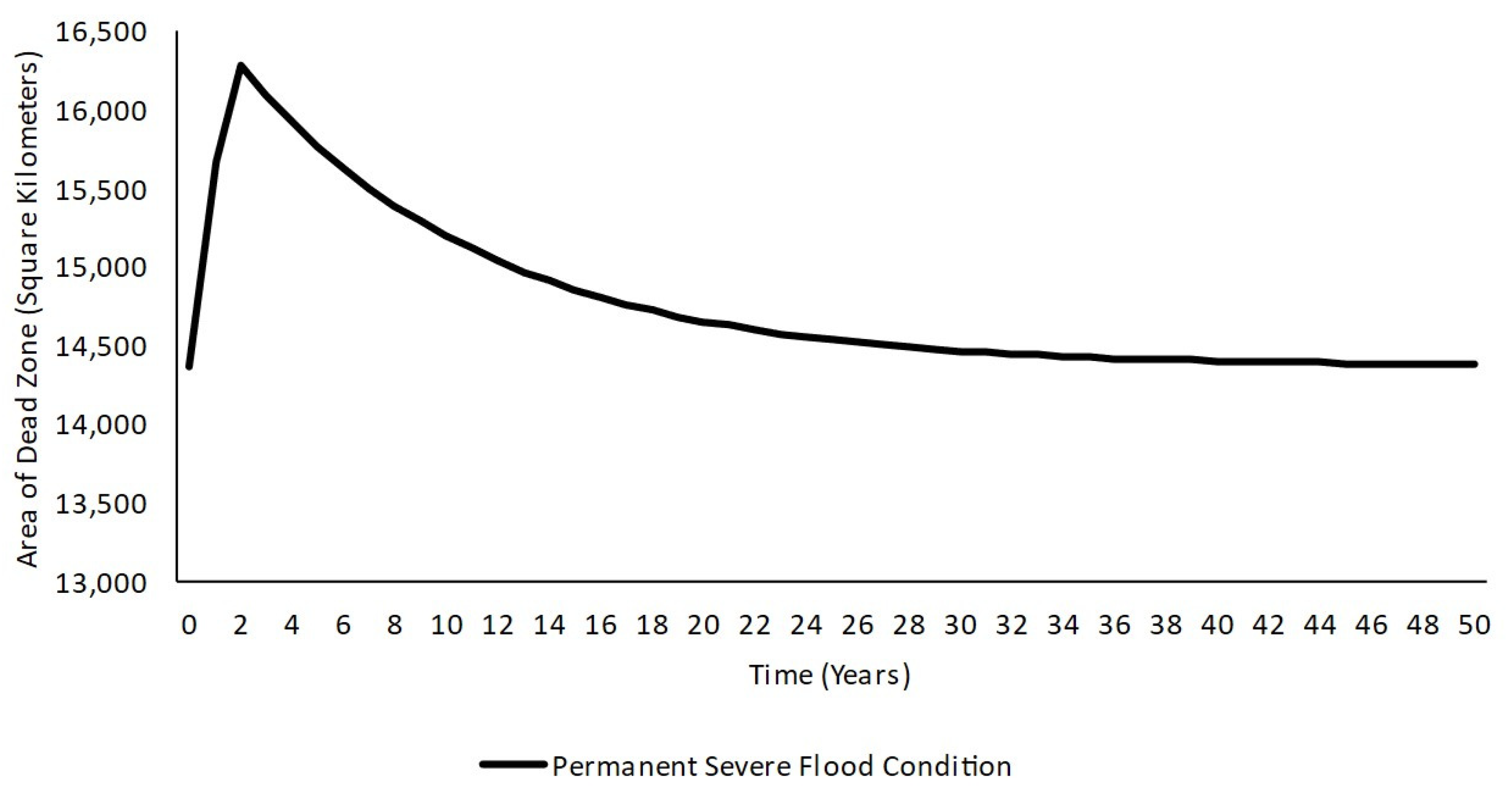
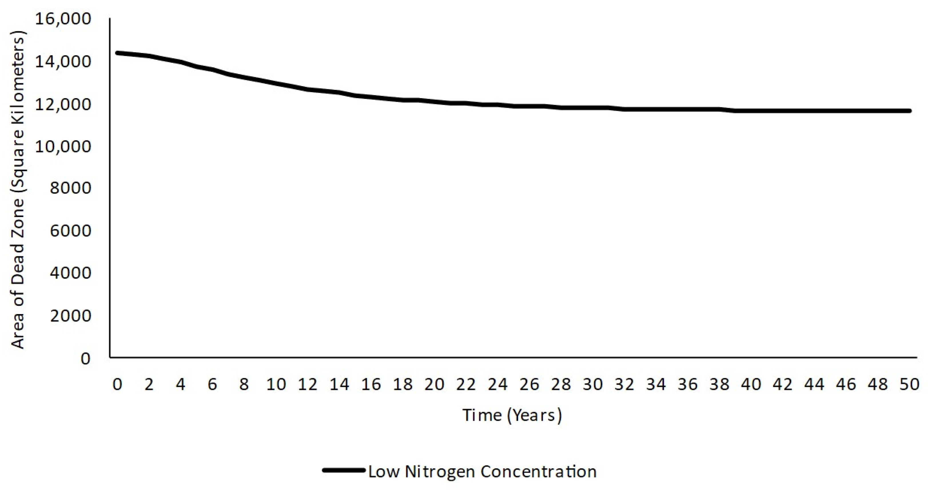
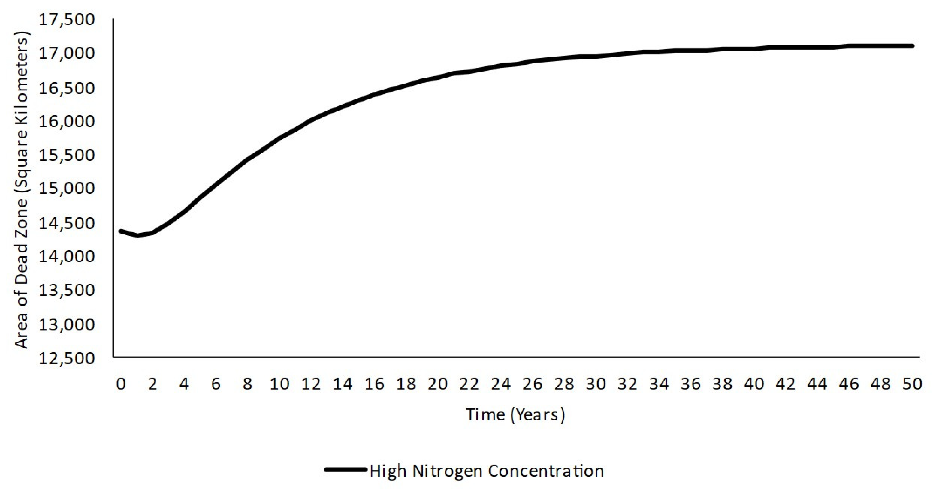
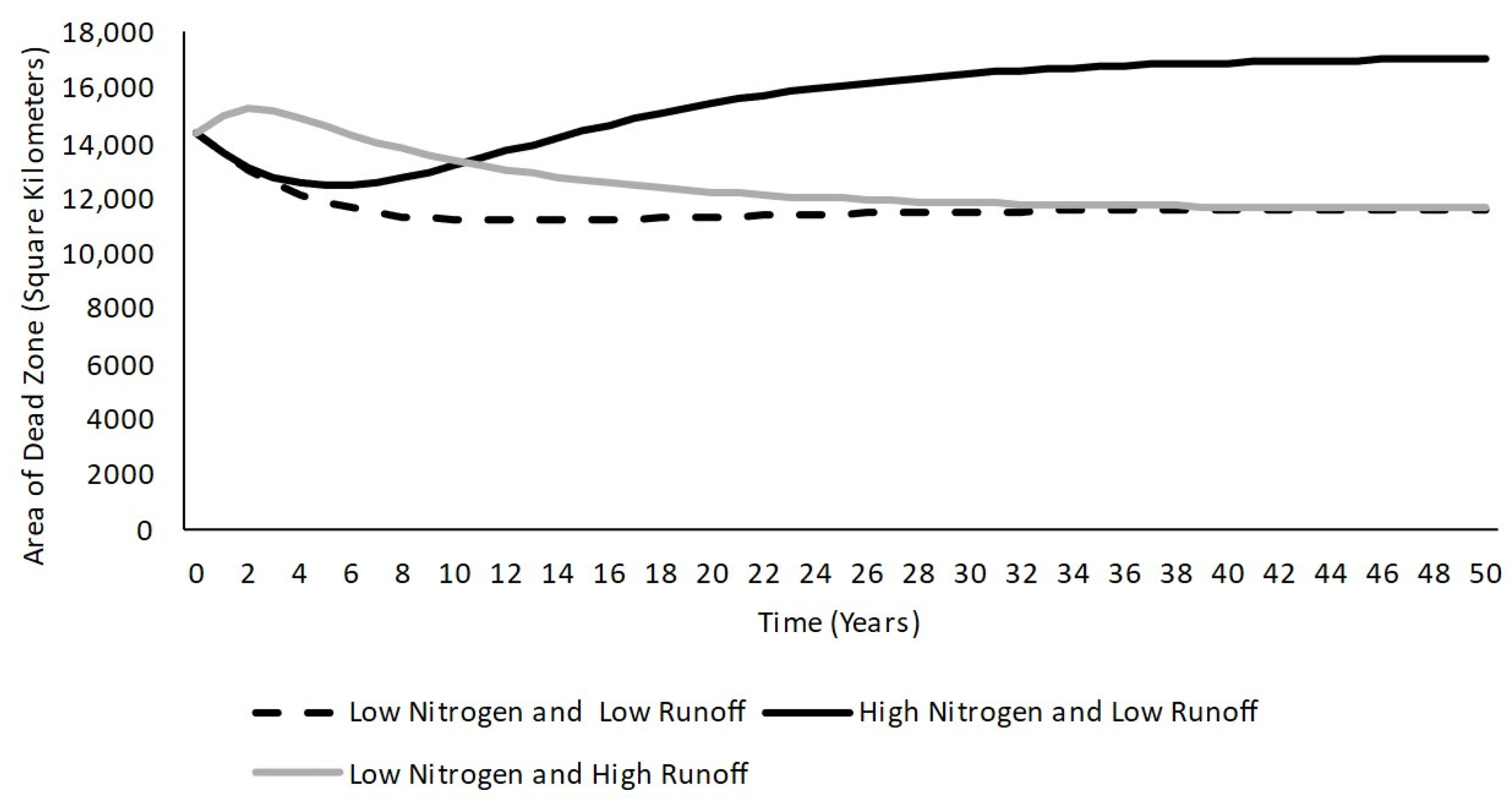
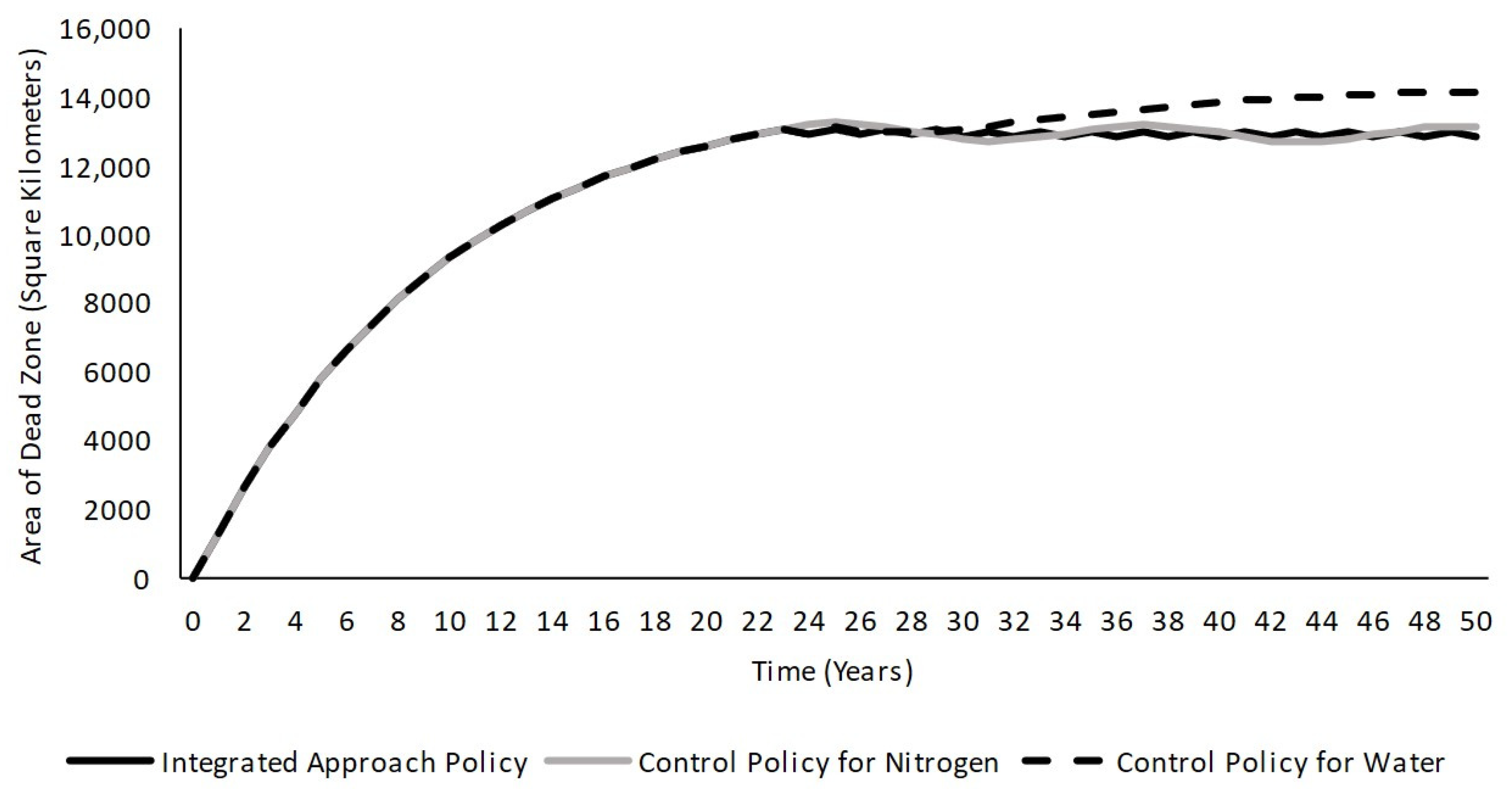
Disclaimer/Publisher’s Note: The statements, opinions and data contained in all publications are solely those of the individual author(s) and contributor(s) and not of MDPI and/or the editor(s). MDPI and/or the editor(s) disclaim responsibility for any injury to people or property resulting from any ideas, methods, instructions or products referred to in the content. |
© 2024 by the authors. Licensee MDPI, Basel, Switzerland. This article is an open access article distributed under the terms and conditions of the Creative Commons Attribution (CC BY) license (https://creativecommons.org/licenses/by/4.0/).