Abstract
Nowadays, the focus of flow shops is the adoption of customized demand in the context of service-oriented manufacturing. Since production tasks are often characterized by multi-variety, low volume, and a short lead time, it becomes an indispensable factor to include supporting logistics in practical scheduling decisions to reflect the frequent transport of jobs between resources. Motivated by the above background, a hybrid method based on dual back propagation (BP) neural networks is proposed to meet the real-time scheduling requirements with the aim of integrating production and transport activities. First, according to different resource attributes, the hierarchical structure of a flow shop is divided into three layers, respectively: the operation task layer, the job logistics layer, and the production resource layer. Based on the process logic relationships between intra-layer and inter-layer elements, an operation task–logistics–resource supernetwork model is established. Secondly, a dual BP neural network scheduling algorithm is designed for determining an operations sequence involving the transport time. The neural network 1 is used for the initial classification of operation tasks’ priority; and the neural network 2 is used for the sorting of conflicting tasks in the same priority, which can effectively reduce the amount of computational time and dramatically accelerate the solution speed. Finally, the effectiveness of the proposed method is verified by comparing the completion time and computational time for different examples. The numerical simulation results show that with the increase in problem scale, the solution ability of the traditional method gradually deteriorates, while the dual BP neural network has a stable performance and fast computational time.
1. Introduction
The development of artificial intelligence has promoted the digitalization, networking, and intelligence development of the manufacturing industry towards Industry 4.0 [1]. With this background, the production and organization mode of the flow shop has changed greatly [2,3]. On the one hand, the Industrial Internet of Things (IIoT) and edge computing technologies enable the real-time collection and rapid processing of underlying data to meet the requirements of high-quality and efficient production. On the other hand, in the face of fierce market competition, service-orientated manufacturing modes such as mass customization make the characteristics of multi-variety, low volume, and a short lead time particularly prominent. Therefore, numerous operation tasks increase the problem size of the computational scheduling. In a typical flow shop, raw materials are transported by an AGV (Automated Guided Vehicle) from a warehouse to corresponding machines for machining, and then again transported by an AGV to complete the subsequent operations in various resources. The delayed arrival of jobs can result in ineffective waiting at subsequent operations such as in following machines and finally end with extended production cycles. Meanwhile, the frequent transport of jobs between machines makes supporting logistics an indispensable factor to be included in practical scheduling decisions. Effective collaboration between multi-stage production and supporting logistics will prevent potential problems and thereby realize the scheduling of operations on a flow floor [4,5].
With constraints such as the frequent transport of jobs, insertion of urgent orders, and process sequence, it becomes necessary but also very challenging to quickly solve multi-stage production and supporting logistics scheduling problems in real-time in a digital-twin flow shop. In recent years, scholars have proposed the use of a complex network theory to solve issues, such as collaborative modeling problems [6], due to its advantages of describing the two-dimensional topology structure of complex manufacturing systems and parameters such as the node degree, clustering coefficient, and redundancy, and thereby the possibility of deriving heuristic information for scheduling rules. However, the above complex network-based models are built based on jobs or operations, but they lack the description of heterogeneous features and correlations among various elements (machine tools, AGVs, jobs). In this case, a supernetwork model consisting of multiple layers of complex networks becomes interesting for representing the multi-layer and multi-attribute characteristics of production logistics in a flow shop [7]. In addition, numerous experiments and operational practices have demonstrated that optimal scheduling results have similarities in machine selection and operation sequencing when similar scheduling problems have been repeatedly solved, while traditional flow shop scheduling algorithms often ignore the historical scheduling data and decisions [8,9]. With the deployment of IIoT and edge computing, large amounts of real-time and historical data can be collected on the flow shop floor to provide inputs for machine learning to efficiently solve real-time scheduling decisions for subsequent jobs.
Motivated by the above background, this paper adopts the supernetwork theory to describe the production and logistics of digital-twin flow shops. As a result, machines, jobs, and buffer sites are mapped as nodes; and the inter/intra-layer process relationships between nodes are mapped as superedges, such as process sequence relationships and machine conflict relationships. Meanwhile, a dual back propagation (BP) neural network is used to establish a scheduling model aiming at improving solving efficiency. The main contributions of this paper are as follows:
- (1)
- An operation task–logistics–resource supernetwork model was introduced to describe the hierarchical and heterogeneous relationships between the production and logistics nodes in a flow shop. The topological feature parameters of this model are extracted and used as inputs for the scheduling algorithm.
- (2)
- A dual BP neural network scheduler was designed to enable the flow shop to make rapid decisions based on the historical optimal scheduling scheme. Specifically, the neural network 1 is used to prioritize operation tasks and generate a priority queue, while the neural network 2 is used to resolve conflicts within the priority queue to form the final scheduling decision.
The rest of the paper is organized as follows. Section 2 reviews the related literature. Section 3 describes the problem of hybrid scheduling on the flow shop. Section 4 deduces the supernetwork modeling for flow shop production logistics. Section 5 establishes a neural network scheduler. Section 6 presents the flow shop scheduling case and its solutions. The conclusions are given in Section 7.
2. Literature Review
The flow shop scheduling problem is a popular research topic in both academia and industry. Current scheduling solution methods mainly include mathematical models, scheduling rules, and meta-heuristic and machine learning. Scheduling methods based on classic mathematical models include branch-and-bound [10] and Lagrangian relaxation [11], among others, which can derive the optimal solution, but the solution often takes a substantial amount of computational time. Rule-based scheduling, e.g., SPT (Shortest Machining time), see [12], EDF (Earliest Deadline First), see [13], LPT (Longest Machining time), see [14], is simple and fast in the solution process, but it has poor generalization ability and tends to be applicable to specific scheduling scenarios [15]. Therefore, meta-heuristic scheduling methods, such as genetic algorithms [16], particle swarm algorithms [17], ant colony algorithms [18], and the frog-leaping algorithm [19], have attracted extensive attentions over the past decades for their ability to find near-optimal solutions through iterative searches within the feasible solution domain. While these algorithms are effective at obtaining optimal solutions, they often require considerable time to solve large-scale scheduling problems.
In recent years, machine learning has demonstrated significant advantages in addressing large-scale scheduling problems [20]. On the one hand, because neural networks can effectively learn from historical data, the computational time required to solve a problem can be significantly reduced, enabling rapid solutions. On the other hand, neural network models can be trained to address other scheduling problems of a similar type and scale. For example, ref. [21] adopted an improved Deep Q-Network (DQN) to implement a scheduling scheme for establishing a robot-driven sanding processing line, aiming to minimize the total delay of multiple parallel service streams. Ref. [22] developed a neural network-based job shop scheduling model that evaluated different possible scheduling schemes based on internal or external constraints. Ref. [23] established a dynamic flexible workshop scheduling problem (DFJSP) model with the goals of maximum completion time and robustness, and used a two-stage algorithm based on convolutional neural networks to solve it. Ref. [24] proposed a multi-layer neural network model for solving the flow shop scheduling problem, presenting the optimal sequence of jobs with the objective of minimizing the makespan. Ref. [25] designed state features, actions, and reward functions by using reinforcement learning algorithms to solve the flow shop scheduling problem, minimizing the completion time. Ref. [26] summarizes the architecture and process of training deep reinforcement learning scheduling models and applying result scheduling solvers. It is widely acknowledged that machine learning can achieve significant improvements in efficiency; however, challenges remain in selecting appropriate input parameters. For instance, operation tasks typically include only basic input parameters, such as the processing time and remaining time, while neglecting features like the correlation between multi-stage production and supporting logistics. Consequently, the potential benefits of applying machine learning to complex scheduling problems remain underexplored. This paper, therefore, employs supernetwork theory with a multi-layer structure to model multi-stage production and supporting logistics in a flow shop. The topological parameters of this model are then incorporated into the input parameters of a neural network to inform practical scheduling decisions. Thus, this study introduces a novel approach to applying machine learning in scheduling problems.
3. Problem Description and Mathematical Model
In this paper, the flow shop scheduling problem integrated with transport times is investigated. Specifically, there are n jobs to be processed on m machines, each job with j operations, and each operation is realized on a specified machine. The scheduling decision is to determine the sequence of the operation and start time on each machine to obtain the optimal scheduling performance. The flow shop contains various jobs, different machines, buffer sites, and AGVs (Automatic Guided Vehicles). According to the MES (Manufacturing Execution System), the operation sequences of each job can be extracted, and the machines corresponding to operations are defined. The following assumptions are made:
- (1)
- All jobs and machines are available at time 0;
- (2)
- Each machine can only process one operation at a time;
- (3)
- Each job can only be processed on one machine at the same time;
- (4)
- Resource interruption can be ignored;
- (5)
- There are sequence constraints between the different operation tasks of a job, and a job needs to go through predefined operation tasks, which can be realized by dedicated machines;
- (6)
- An AGV is sufficient to complete the transport task;
- (7)
- Transport time dominates; therefore, the loading and unloading time can be ignored.
Table 1 shows the notations to be used for the model.

Table 1.
Mathematical notations.
Considering minimizing the maximum completion time (makespan), the mathematical model is expressed as follows:
4. Supernetwork Modeling for Flow Shop Production Logistics
Selecting the appropriate input parameters is one critical problem in improving the performance of machine learning-based scheduling models. Currently, the commonly used parameters, such as the processing time and remaining time, often lead to incomplete scheduling scheme information. With this background, the supernetwork theory based on a multi-layer complex network is used to describe the flow shop production and logistics settings.
4.1. Analysis of Flow Shop Production Logistics Elements
This section analyzes the flow shop production and logistics elements from the network perspectives of the “node” and “edge”. From the perspective of the “node”, the flow shop elements include machines, buffer sites, and jobs. From the perspective of the “edge”, the links between nodes include the processing relationship and the transport relationship. Specifically, the processing relationship refers to the multi-stage operations that convert raw materials into finished products [27], and the transport relationship refers to the jobs’ movement between two nodes (machines or buffer site) by using AGVs. Therefore, jobs are the core carrier of edges in the flow shop production logistics.
4.2. Supernetwork Model Construction and Feature Extraction
4.2.1. Supernetwork Model Construction
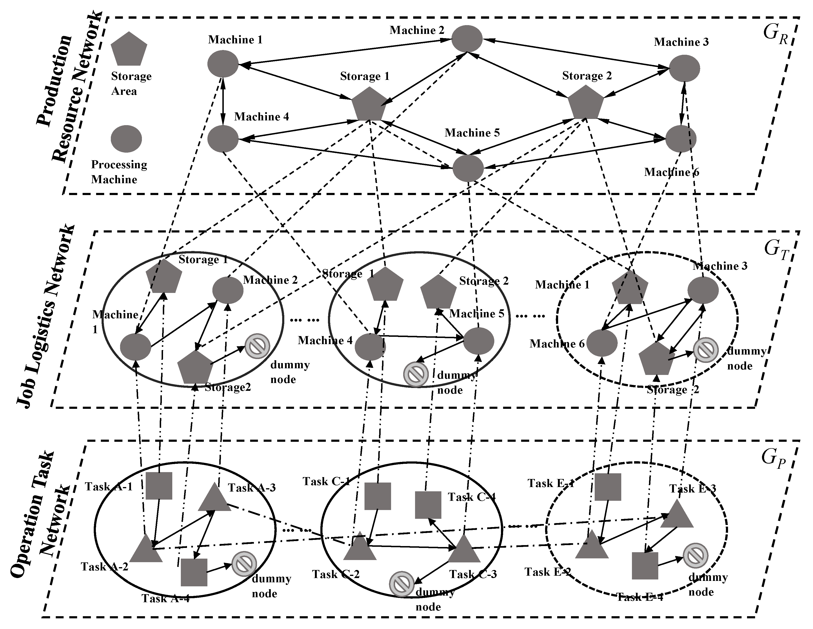
The supernetwork based on a multi-layer complex network is a collection of multiple single-layer subnets. Therefore, it is essential to analyze the correlation relationship between different sub-networks and map them into superedges. As shown in Figure 1, we establish an operation task–logistics–resource supernetwork model, and each sub-network is abstracted into a weighted directed complex network G = {V, E, w}.
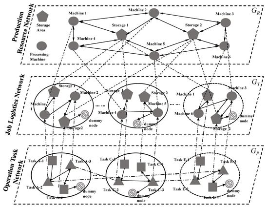
Figure 1.
Operation task–logistics–resource supernetwork model.
The supernetwork model includes three parts: operation tasks, job logistics, and production resources. Each part includes nodes, edges between nodes on the same layer, and edges between nodes on different layers, and together these elements describe the multi-layer networked relationships of flow shop production logistics.
The specific description of each sub-network model is shown in Table 2. GR reflects the logical layout of machines and their buffer sites in a flow shop; GT reflects the material handling based on the operation tasks; and Gp reflects the relationships between machining tasks and transport tasks.
Table 2.
The definitions of each sub-network.
Based on the above three sub-networks models, the operation task–logistics–resource supernetwork model can be represented by triples
where ERT and ETP, respectively, represent the inter-layer connected edges between sub-networks GR and GT and between sub-networks GT and GP, which are called superedges. The meanings are specified as follows:
- (1)
- The superedge between sub-networks Gp and GT is EPT, which represents the mapping of nodes in the operation task layer sub-network to the machines used by the operation task.
- (2)
- The superedge between sub-networks GT and GR is ERT, which represents the mapping between the nodes in the job logistics layer sub-network (that is, the machines used by the operation tasks involved in the operation task layer network nodes) and the machine nodes in the actual flow shop. Here, the machining and transport operations of operation tasks are separated into two layers of networks, which makes the machining and transport operations easier to analyze. It is also one of the major advantages of using a supernetwork to describe complex systems.
4.2.2. Supernetwork Feature Knowledge Extraction
The objective of flow shop production logistics is to minimize the maximum completion time. There is a mapping relationship between the supernetwork characteristics and the scheduling objectives, as explained as follows:
- (1)
- The job operation number Ni can be determined by the node sequence of the operation tasks layer network, which can be directly used as input information for subsequent neural networks.
- (2)
- According to the network edge’s definition of the operation tasks layer, the edge weight wp between the current operation task node and the next operation task represents the time for completing the current operation task.
- (3)
- The out-degree of network nodes can be obtained from the job logistics layer network. The out-degree OLDP of nodes in the operation tasks logistics layer network represents the time of logistics transport between nodes due to operation tasks.
- (4)
- The high-order out-degree HODP of the operation tasks layer network reflects the sum of processing times for the next operation tasks in the current process, i.e., the sum of the remaining processing times.
- (5)
- The node degree Dp of the operation tasks layer network: The node degree of the operation task layer reflects the number of tasks associated with the current operation task and the degree of correlation between the task node and other nodes in the network. This attribute is one of the most important topology attributes in the supernetwork, and a large value of Dp indicates the high impact of the task node.
- (6)
- The node degree DR of the production resource layer network: the node degree of machines reflects the number of resources associated with current machines, and it reflects the importance of the machines in the production resources network.
- (7)
- The node clustering coefficient CR of the production resources layer network: the clustering coefficient of machine nodes affects the propagation dynamics on the network, and it reflects the importance of machines’ connection in the production resources layer network.
- (8)
- The comprehensive loss LR of machines can affect the normal running life and failure probability, and it affects the completion time of the operation tasks. Therefore, the comprehensive loss is added as the attribute to characterize the fault of machines. The combined loss is equal to the product of the processing time undertaken by the machine and the loss per unit of time.
5. Establishment of Neural Network Scheduler
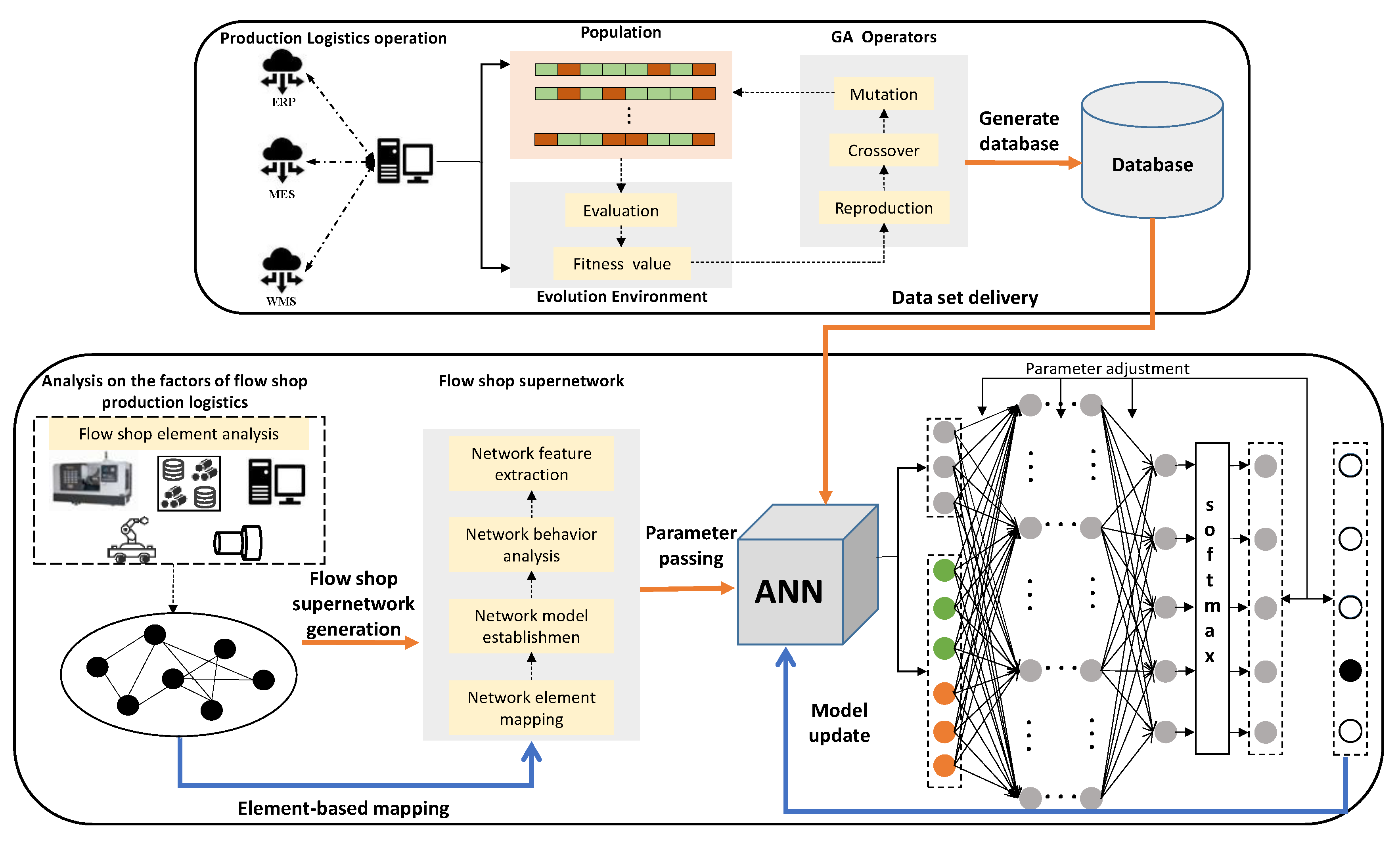
The topological features of the supernetwork model in Section 4.2.2 can be utilized to provide the input parameters to the BP neural network model. This hybrid approach has obvious advantages in real-time, generalization, and data mining for flow shop scheduling problems. As shown in Figure 2, a hybrid scheduling method based on a dual BP neural network includes the following steps. First, the above problem considering the transport time is solved by a genetic algorithm to obtain the optimal scheduling sequence and generate the data set to solve the neural network training data set. Secondly, the network attributes related to scheduling are selected as the input parameters of the neural network by combining them with the supernetwork theory. Finally, an integrated neural network model is established and the two neural networks are trained using the data set. The trained neural networks are used to classify the operational priorities of each job in the new scheduling problem to obtain the final solution.
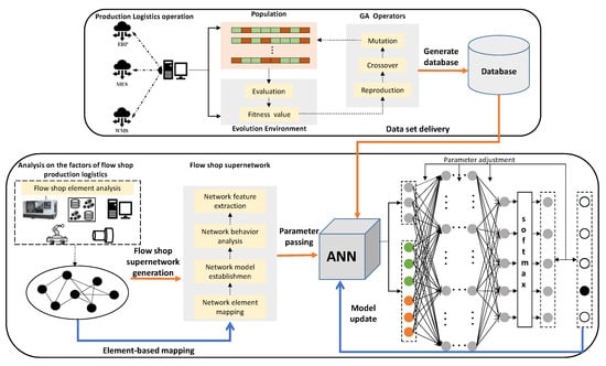
Figure 2.
Neural network scheduler diagram.
5.1. Selection and Transformation of Neural Network Input Parameters
The neural network 1 is used to preliminarily classify all operation tasks. Considering the characteristics of a scheduling problem, some traditional attributes of the operation tasks [28] and attributes extracted from the operation task–logistics–resource supernetwork are selected as the input parameters of the neural network 1, as follows: the node serial number in the operation tasks layer network, node out-degree in the operation tasks layer network, node out-degree in the job logistics layer network, high-order out-degree of nodes in the operation tasks layer network, node degree in the operation tasks layer network, node degree in the production resources layer network, clustering coefficient in the production resources layer network nodes, and the comprehensive loss in the production resources layer.
The neural network 2 aims to sequence the operations of conflicting tasks. Such conflicting tasks are caused by operation constraints and machine constraints. On the one hand, there are sequence constraints between the different operation tasks of a job; on the other hand, several tasks may share and compete for one machine, which creates conflicts among tasks, and it is important to determine the exact machining sequences. If there are several conflicting tasks in the flow shop scheduling, we assign all conflicting tasks into groups, with each containing at most two operation tasks. Further, the operations sequence of two conflicting tasks is subdivided based on the priority division of the neural network 1, which compares and classifies the input parameters in the neural network 1. Therefore, the input properties of neural network 2 can be described as follows: each attribute in neural network 1 is used as a comparison item to compare each attribute of the conflict tasks.
5.2. Selection and Transformation of Neural Network Output Parameters
As the size of the scheduling problem increases, sequencing the conflicting operations can greatly increase the computational time. Therefore, this section uses a dual BP neural network to schedule all tasks in the operations sequence. The neural network 1 is trained to initially prioritize the tasks, and the neural network 2 is trained to rank conflicting tasks with the same priority. This approach can effectively reduce the computational time and accelerate the solution process. In neural network 1, the priority is initially divided into six levels, while in neural network 2, the priority is divided into two levels.
5.3. Structure of Neural Network Scheduler
BP neural networks 1 and 2 contain an input layer, output layer, and hidden layer. It is necessary to determine the number of nodes in each layer to establish the neural network model.
(1) Input layer. According to Section 5.1, the input layer of BP neural network 1 consists of eight basic parameters and the input layer of BP neural network 2 consists of eight basic parameters. The number of nodes in the neural network input layer is determined according to the number of codes corresponding to each basic parameter.
(2) Output layer. The output targets of BP neural network 1 are initially determined as six priorities, so there are six output nodes. The output target of BP neural network 2 is the conflict process sequence, and the corresponding results can only be pre-processing and post-processing; that is, the number of corresponding output nodes is two.
(3) Hidden layer. The number of hidden nodes in the BP neural network is determined by an empirical formula. The number of nodes in the hidden layer has an important influence on the classification accuracy and computational complexity of the neural network. The initial number of hidden layer nodes can be determined by empirical formulas [29]. For example, , where n1 is the number of hidden nodes, n is the number of inputs, m is the number of outputs, and a is between 1 and 10. In this paper, the number of nodes in the hidden layer of the BP neural network 1 is preliminarily set as 6–16, and the number of nodes in the hidden layer of the BP neural network 2 is selected as 4–16. Ultimately, the number of nodes in the hidden layer needs to be repeatedly debugged to find the optimal solution.
6. Numerical Examples
The algorithm is programmed by Matlab R2018b and runs on PC with Intel G5400 CPU, 3.70 GHZ main frequency, and 4 GB memory. UCINET 6 software is used to establish and analyze the model for the operation task–logistics–resource supernetwork.
6.1. Construct the Training Data Set
The training process of the neural network is to discover the rule of the data set. For example, the optimal scheduling result sets are similar, so the neural network model can be used to train for mining the optimal scheduling scheme data set. However, the scheduling scheme cannot be directly used as the training data of the neural network. Instead, the corresponding input parameters should be used to describe the scheduling information reflected in the scheduling scheme, so as to transform the scheduling scheme into a training data set and obtain the corresponding binary coding to form the input set of training samples. At the same time, the position of each task in the sequence is transformed into the priority and used as the target output to obtain the output set of the training sample composed of 6-bit binary codes.
In this section, based on the problem model in Section 3, a genetic algorithm is first used to solve the flow shop scheduling problem considering the transport time to obtain the optimal set of scheduling solutions as the training data set for the neural network. The parameters of the genetic algorithm are set as follows: number of individuals = 40; maximum number of generations = 500; selection rate = 0.9; crossover rate = 0.8; and mutation rate = 0.6. Considering the transport time of jobs between the buffer site and machines, as well as between different machines, the tasks and corresponding time of the flow shop scheduling problem are shown in Table 3. The case consists of 8 machines, 2 buffer sites, and 6 jobs, each of which contains 6 process tasks, outbound and inbound tasks. The corresponding numbers of machines are 1–8, and the corresponding numbers of buffer sites are 9 and 10, respectively, and the numbers of the AGVs are 11–16, respectively. Here, the AGVs are assigned with the order strategy, where the transport tasks during the jobs’ machining are executed from start to finish by the defined AGV.
Table 3.
Flow shop scheduling case considering transport time (Time unit: min).
For the pair values in Table 3, the first indicates the machine, AGV, or storage area number used for the operation task; and the second indicates the processing time, transport time, and inbound and outbound time associated with the storage area, respectively. For example, in the row Process 1 and column job A, (3, 1) denotes that operation task 1 of job A is machined by machine 3, and its processing time is 1 min; the route of 1st job includes (Buffer site-10) → (Machine-3) → (AGV-11) → (Machine-1) → (AGV-11) → (Machine-7) → (AGV-11) → (Machine-4) → (AGV-11) → (Machine-8) → (AGV-11) → (Machine-5) → (Buffer site-9).
6.2. Supernetwork Topology Feature Extraction
The topological characteristics of the flow shop production logistics can be used as input parameters to train the neural networks. Firstly, according to the establishment method of the operation task–logistics–resource supernetwork model, the adjacency matrix of each layer network is obtained in Appendix A. The specific construction method is as follows:
- (1)
- If there is no edge relation between the two nodes, the value at the corresponding position in the adjacency matrix is 0.
- (2)
- If there is an edge relation between the two nodes, the value at the corresponding position in the adjacency matrix is not 0. The values in the network adjacency matrix of the operation tasks layer represent the processing time between the start node and the end node (0.01 means there is an adjacency relationship, but it is an incoming and outgoing task, so the processing time is ignored). The values of the network adjacency matrix of the job logistics layer represent the logistics transport time between the start node and the end node. The values in the network adjacency matrix of the production resources layer represent the logistics transport time between the start node and the end node.
According to the adjacency matrix and each network model, UCINET software can be used to obtain the network model diagram of the operation task layer and the network topology characteristics of each node, as shown in Table 4. Since the outbound and inbound tasks do not affect the scheduling sequence, only the characteristic attributes of operation tasks other than outbound and inbound tasks are retained in Table 4. All network features in the table, including those of subsequent resource layer nodes, correspond to the attribute description in Section 4.2.2.
Table 4.
Statistics of partial characteristic attributes of operation tasks and logistics layer.
According to the statistics of the network topology characteristics of the operation task and the logistics layer in Table 4, the sequence number, out-degree, high-order out-degree, degree value of each node of the operation task, and the out-degree of the logistics layer node of the corresponding operation task can be obtained. These characteristics reflect the state evaluation of the production process and logistics transport. At the same time, in order to intuitively describe the sequence constraints and resource constraints between conflict operation tasks, the degree value with constraints is set as 0.01. Otherwise, weighted edges cannot be constructed.
According to the machine network adjacency matrix and supernetwork adjacency matrix, the partial network topology characteristics of each node can be obtained. At the same time, according to the determination of China Machines Association in 2015, the average MTBF time of machines made in Germany is 2000 h, and the average MTBF time of machines made in China is 1100 h. Assuming that machines 1, 2, 3, and 4 are made in Germany, and machines 5, 6, 7, and 8 are made in China, the loss rates per unit time can be preliminarily selected as 0.000008% and 0.000017%, respectively. To sum up, the selected network topology features were extracted and counted, and the machine comprehensive loss was calculated based on the superedge attributes of machine nodes. Statistics on the characteristics of machining resources are shown in Table 5.
Table 5.
Statistics of some characteristic attributes of production resource layer.
6.3. Training the BP Neural Network
Firstly, the genetic algorithm is used to solve the procedure sequence of the optimal scheduling scheme under the existing scheduling rules. Secondly, based on the scheduling sequence, processes are classified according to selected input parameters, and data sets are generated. Then, the scheduling data set of the optimal scheduling sequence is selected, and the coding of each operation task and its priority can be obtained according to the coding table and the corresponding coding of each scheduling sequence operation task; that is, the training data set of BP neural network 1 can be obtained. According to the obtained scheduling scheme, the data set is composed, and BP neural network 1 is established. The parameters of BP neural network 1 are set as follows: the input node is 22, the node number of the hidden layer 1 is 20, the node number of hidden layer 2 is 10, the node number of the output layer is 6, the learning rate is 0.0001, and the maximum convergence algebra is 1000.
The confusion matrix shows the training results of BP neural network 1 and reflects the accuracy of neural network BP1 in classifying the priority of operational tasks, as shown in Table 6. In the field of machine learning, a confusion matrix is also called a possibility matrix or error matrix. A confusion matrix is a summary of the prediction results of classification problems. It uses the count value to summarize the number of correct and incorrect predictions and subdivides according to each category to obtain accuracy.
Table 6.
Confusion matrix for BP neural network 1.
The values on the diagonal in Table 6 represent the correct times predicted by the neural network for each type of value, for example, for a production task at priority 1. In the test example, the number of times that the production task is classified to priority 1 is 2665, the number of times that it is classified to priority 2 is 335, and the number of times that it is classified to priorities 3, 4, 5, and 6 is 0. Therefore, the number of correct classifications was 2665, and the prediction accuracy of the procedure with priority 1 was 2665 in proportion to all the prediction times. At the same time, the classification accuracy rate of the neural network for each category and the overall classification accuracy rate are given in Table 6.
Similar problems have been solved in previous studies. For example, in the paper of a flow shop scheduling algorithm based on an artificial neural network [30], the classification accuracy of the BP neural network model is 70%, while in the paper on neural network scheduling based on complex network features [31], the classification accuracy of a BP neural network is 76.2%. Compared with these papers, we added topological feature indexes of the supernetwork, which made the neural network model describe the scheduling process more comprehensively, and further improved the training results.
In order to further determine the scheduling sequence, BP neural network 2 can be used for training again after the priority division of all processes is realized by BP neural network 1. The parameters of neural network 2 are set as follows: the input node is 24, the number of nodes in the hidden layer is 16, the number of nodes in the output layer is 2, the learning rate is 0.00001, and the maximum convergence algebra is 1000. Table 7 shows the training results of BP neural network 2, which reflect the accuracy for priority classification of conflicting tasks and the overall classification accuracy.
Table 7.
Confusion matrix for BP neural network 2.
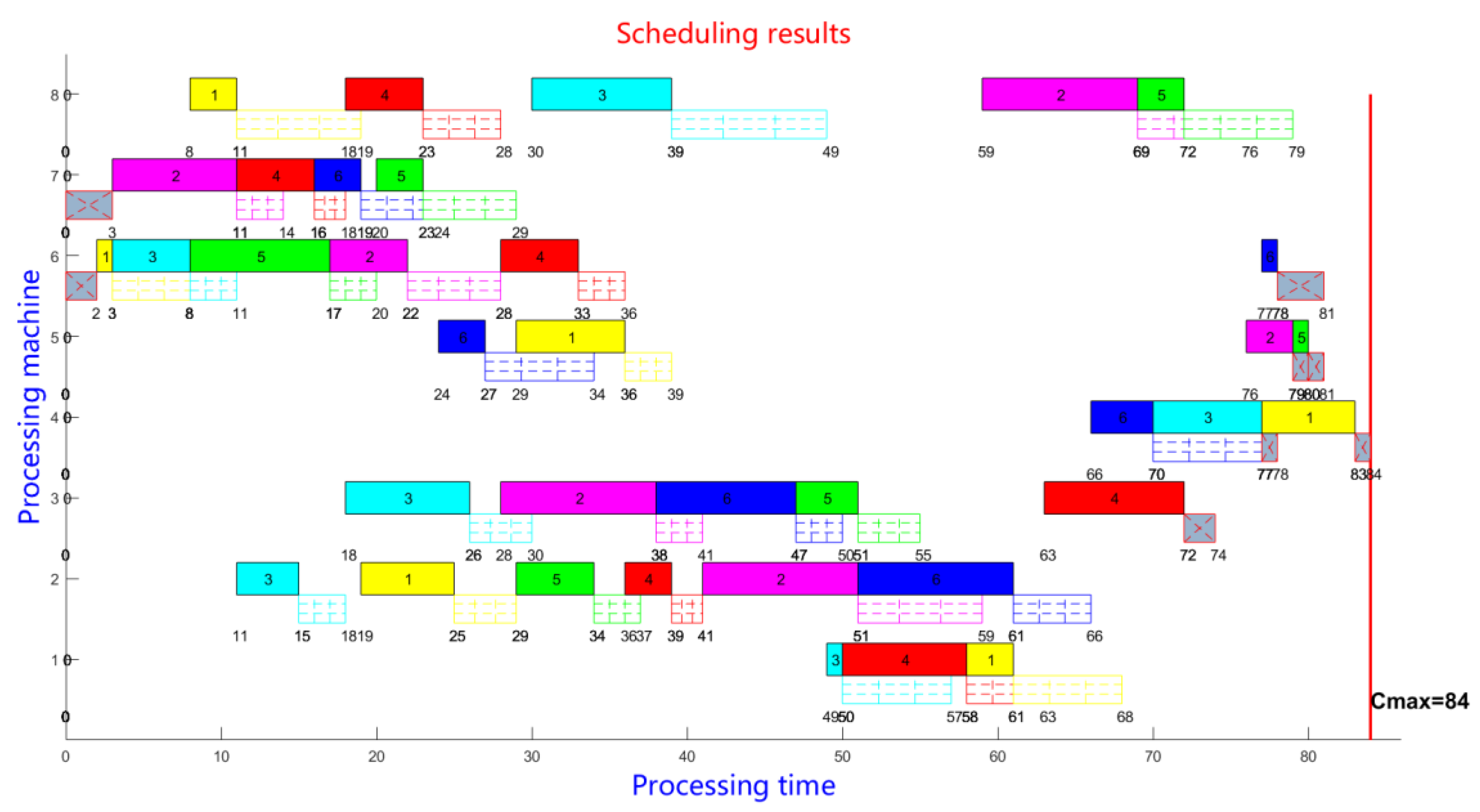
By using BP neural network 1 and BP neural network 2, the maximum completion time of the scheduling scheme is 84 according to the sequencing results of each operation task of the flow shop scheduling problem, with the consideration of the transport time. Scheduling Gantt charts can be generated based on scheduling sequences, as shown in Figure 3, in which the number represents the start and end time of operation tasks and logistics transport links. The logistics transport link includes the logistics tasks involving warehouses and production links. Among them, the gray squares crossed by dashed lines denote the logistics of the warehouse link; The squares filled with dashed lines denote the logistics of the production links. Operation tasks are represented by colored squares.
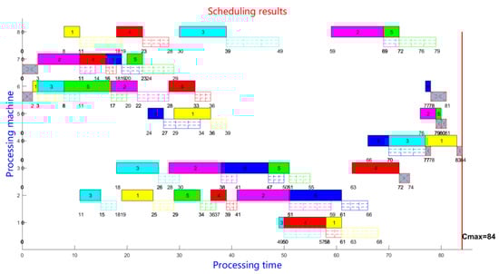
Figure 3.
Flow shop scheduling results generated by dual BP neural networks.
6.4. Experimental Comparison
To verify the performance of the dual BP neural network and compare with other optimization methods, we use three sets of flow shop scheduling problems considering transport time, with 100 iterations of each method in the experiments. To better reflect the pattern of six algorithms (GA/PSO/SA/LPT/SPT/Dual BP) in finding the optimal solution, the completion time and computational times of 100 iterations are computed. The first set of flow shop scheduling cases FT06 includes 8 machines, 6 jobs, and 6 operation tasks for each job; the second set of flow shop scheduling cases LA01–LA05 has 13 machines, 10 jobs, and 10 operation tasks for each job; and the third set of flow shop scheduling cases LA26–LA30 has 13 machines, 20 jobs, and 10 operation tasks for each job. Table 8 shows the completion time of each algorithm, and Table 9 shows the computational time of each algorithm.
Table 8.
Comparison of scheduling solution results (Unit: min).
Table 9.
Comparison of computational time (Unit: s).
Based on both Table 8 and Table 9, it can be seen that scheduling with a dual BP neural network will result in a shorter completion time and a shorter computational time, and its optimization results (completion time) have a higher stability compared with other algorithms. Although the genetic algorithm can sometimes obtain a good value in the objective function, the results are unstable. In fact, the genetic algorithm has a poor performance on average, and it takes a much longer computational time. Although particle swarm optimization and simulated annealing particle swarm optimization end with relatively stable results in terms of the completion time, these two approaches are difficult to obtain the optimal results because the solution procedures often lead to local minimum. Although the computational time of traditional SPT and LPT scheduling rules is short, these scheduling rules are restrictively applicable to a simple scheduling environment and lack the consideration of multiple factors in the multi-scheduling process. For example, SPT and LPT only consider the processing time of each production task and cannot take into account the transport time of logistics.
Meanwhile, comparing the experiments of different problem scales, it can be seen that the dual BP neural network model introduced in this paper outperforms other scheduling rules in solving the flow shop scheduling problem considering the transport time. Moreover, after the BP neural network training is completed, the optimal scheduling results can be obtained with less computational time with new problems of the same scale, especially in cases where the problem scale becomes larger. Actually, this is the challenging case for the traditional scheduling methods, as the associated computational time increases sharply or the solution quality deteriorates quickly; therefore, their application becomes questionable in reality. Although it takes some time to train the model of the BP neural network, it is not necessary to re-train the network model for each new problem computation, and the scheduling solution can be generated based on the trained model. In summary, the BP neural network scheduler can obtain a better solution in a short time with good feasibility.
7. Conclusions
Taking flow shop production and logistics operations as the object, we have established a scheduling model by integrating the supernetwork and neural network. The genetic algorithm is used to solve the flow shop scheduling problem considering the transport time to obtain the data set, and the key topological characteristics have been extracted as part of the input parameters for the neural network.
(1) Based on the hierarchical relationship and heterogeneous relationship between the node elements in the flow shop production and logistics, an operation task–logistics–resource supernetwork model based on the multi-layer complex network is developed. Machines, jobs, and buffer sites are mapped as nodes, and the in-layer/inter-layer correlations between nodes are mapped as the superedge. It overcomes the shortcomings of traditional models in analyzing the relationship between heterogeneous elements and also improves the hierarchical analysis in modeling complex networks.
(2) We have designed the dual BP neural network scheduling model of the flow shop production logistics. The supernetwork features are extracted into input parameters, such as the node degree, node strength, and clustering coefficient. In the numerical example, three sets of flow shop scheduling problems considering the transport time are tested by six algorithms. The results show that the dual BP neural network model has a better performance in terms of completion time and computational time, and, moreover, it has a higher stability than other algorithms. The construction of the operation task–logistics–resource supernetwork model presents a comprehensive perspective. It takes into account the correlations between the different layers of factors that affect the operation of the flow shop production logistics. Therefore, the supernetwork model improves the classification accuracy of the neural network. Meanwhile, unlike other intelligent algorithms that solve the problem iteratively from initial solution to optimal solution, the dual neural network scheduling can meet the requirements of real-time scheduling in the flow shop by learning from historical optimal data.
The paper has proposed a scheduling method combining supernetwork and neural networks, and it provides a new way to solve the flow shop production logistics. The superiority of the above method mainly depends on the completeness and balance of the training data obtained by the genetic algorithm and the more accurate input parameters provided by the operation task–logistics–resource supernetwork. Therefore, further consideration can be given to establishing corresponding databases and rules for each scheduling stage, or to consider algorithms such as KKT (Karush–Kuhn–Tucker) to obtain a more comprehensive sample set. In addition, we can extend the dual BP neural networks scheduling model to consider processes with flexible resources (machines) for another type of flexible scheduling problem.
Author Contributions
H.M. and Z.W. wrote the paper; S.W. provided the funding acquisition; G.Z. collected the related data; J.C. developed a software testing system; F.Z. provided the research idea. All authors have read and agreed to the published version of the manuscript.
Funding
This work was supported in part by the China University Industry University Research Innovation Fund (No. 2020ITA04008). In addition, the authors also would like to thank Ou Tang of Linköping University, Sweden, for his valuable comments and constructive criticism.
Data Availability Statement
Data are contained within the article.
Conflicts of Interest
The authors declare no conflicts of interest.
Appendix A
Table A1 shows the adjacency matrix of each layer network in the operation task–logistics–resource supernetwork model.
Table A1.
Network adjacency matrix of production resources layer.
Table A1.
Network adjacency matrix of production resources layer.
| Resources | Machine 1 | Machine 2 | Machine 3 | Machine 4 | Machine 5 | Machine 6 | Machine 7 | Machine 8 | Buffer 1 | Buffer 2 |
|---|---|---|---|---|---|---|---|---|---|---|
| Machine 1 | 0 | 2 | 0 | 0 | 0 | 0 | 0 | 0 | 2 | 0 |
| Machine 2 | 2 | 0 | 3 | 0 | 0 | 3 | 0 | 0 | 3 | 0 |
| Machine 3 | 0 | 3 | 0 | 2 | 0 | 0 | 3 | 0 | 0 | 2 |
| Machine 4 | 0 | 0 | 2 | 0 | 0 | 0 | 0 | 0 | 0 | 1 |
| Machine 5 | 0 | 0 | 0 | 0 | 0 | 2 | 0 | 0 | 1 | 0 |
| Machine 6 | 0 | 3 | 0 | 0 | 2 | 0 | 3 | 0 | 2 | 0 |
| Machine 7 | 0 | 0 | 3 | 0 | 0 | 3 | 0 | 2 | 0 | 3 |
| Machine 8 | 0 | 0 | 0 | 0 | 0 | 0 | 2 | 0 | 0 | 2 |
| Buffer 1 | 2 | 0 | 0 | 0 | 1 | 0 | 0 | 0 | 0 | 0 |
| Buffer 2 | 0 | 0 | 0 | 1 | 0 | 0 | 0 | 2 | 0 | 0 |
References
- Zheng, T.; Ardolino, M.; Bacchetti, A.; Perona, M. The applications of industry 4.0 technologies in manufacturing context: A systematic literature review. Int. J. Prod. Res. 2021, 59, 1922–1954. [Google Scholar]
- Liu, W.H.; Hou, J.H.; Yan, X.Y.; Tang, O. Smart logistics transformation collaboration between manufacturers and logistics service providers: A supply chain contracting perspective. J. Manag. Sci. Eng. 2021, 6, 25–52. [Google Scholar] [CrossRef]
- Winkelhaus, S.; Grosse, E.H. Logistics 4.0: A systematic review towards a new logistics system. Int. J. Prod. Res. 2020, 58, 18–43. [Google Scholar] [CrossRef]
- Hu, Y.; Wu, X.; Zhai, J.J.; Lou, P.H.; Qian, X.M.; Xiao, H.N. Hybrid task allocation of an AGV system for task groups of an assembly line. Appl. Sci. 2022, 12, 10956. [Google Scholar] [CrossRef]
- Xiao, H.N.; Wu, X.; Qin, D.J.; Zhai, J.J. A collision and deadlock prevention method with traffic sequence optimization strategy for UGN-based AGVS. IEEE Access 2020, 8, 209452–209470. [Google Scholar] [CrossRef]
- Li, Y.F.; Tao, F.; Cheng, Y.; Zhang, X.Z.; Nee, A.Y.C. Complex networks in advanced manufacturing systems. J. Manuf. Syst. 2017, 43, 409–421. [Google Scholar] [CrossRef]
- Nagurney, A.; Dong, J. Supernetworks: Decision-Making for the Information Age; Edward Elgar Publishers: Chelthenham, UK, 2002; pp. 803–818. [Google Scholar]
- Esteso, A.; Peidro, D.; Mula, J.; Díaz-Madroñero, M. Reinforcement learning applied to production planning and control. Int. J. Prod. Res. 2023, 61, 5772–5789. [Google Scholar] [CrossRef]
- Zhou, G.H.; Chen, Z.H.; Zhang, C.; Chang, F.T. An adaptive ensemble deep forest based dynamic scheduling strategy for low carbon flexible job shop under recessive disturbance. J. Clean. Prod. 2022, 337, 130541. [Google Scholar] [CrossRef]
- Ahn, J.; Kim, H.J. A branch and bound algorithm for scheduling of flexible manufacturing systems. IEEE Trans. Autom. Sci. Eng. 2023, 21, 4382–4396. [Google Scholar] [CrossRef]
- Hajibabaei, M.; Behnamian, J. Fuzzy cleaner production in assembly flexible job-shop scheduling with machine breakdown and batch transportation: Lagrangian relaxation. J. Comb. Optim. 2023, 45, 112. [Google Scholar] [CrossRef]
- Leu, J.S.; Chen, C.F.; Hsu, K.C. Improving heterogeneous SOA-based IoT message stability by shortest processing time scheduling. IEEE Trans. Serv. Comput. 2014, 7, 575–585. [Google Scholar] [CrossRef]
- Kruk, L.; Lehoczky, J.; Ramanan, K.; Shreve, S. Heavy traffic analysis for EDF queues with reneging. Ann. Appl. Probab. 2011, 21, 484–545. [Google Scholar] [CrossRef]
- Della Croce, F.; Scatamacchia, R. The longest processing time rule for identical parallel machines revisited. J. Sched. 2020, 23, 163–176. [Google Scholar] [CrossRef]
- Meng, L.L.; Duan, P.; Gao, K.Z.; Zhang, B.; Zou, W.Q.; Han, Y.Y.; Zhang, C.Y. MIP modeling of energy-conscious FJSP and its extended problems: From simplicity to complexity. Expert Syst. Appl. 2024, 241, 122594. [Google Scholar] [CrossRef]
- Meng, L.L.; Cheng, W.Y.; Zhang, B.; Zou, W.Q.; Fang, W.K.; Duan, P. An improved genetic algorithm for solving the multi-AGV flexible job shop scheduling problem. Sensors 2023, 23, 3815. [Google Scholar] [CrossRef] [PubMed]
- Fontes, D.; Homayouni, S.M.; Gonçalves, J.F. A hybrid particle swarm optimization and simulated annealing algorithm for the job shop scheduling problem with transport resources. Eur. J. Oper. Res. 2023, 306, 1140–1157. [Google Scholar] [CrossRef]
- Zhang, C.Y.; Jiang, P.Y.; Zhang, L.; Gu, P.H. Energy-aware integration of process planning and scheduling of advanced machining workshop. Proc. Inst. Mech. Eng. Part B-J. Eng. Manuf. 2017, 231, 2040–2055. [Google Scholar]
- Meng, L.L.; Zhang, C.Y.; Zhang, B.; Gao, K.Z.; Ren, Y.P.; Sang, H.Y. MILP modeling and optimization of multi-objective flexible job shop scheduling problem with controllable processing times. Swarm Evol. Comput. 2023, 82, 101374. [Google Scholar] [CrossRef]
- Atsmony, M.; Mor, B.; Mosheiov, G. Single machine scheduling with step-learning. J. Sched. 2022, 27, 227–237. [Google Scholar] [CrossRef]
- Yang, Y.Q.; Chen, X.; Yang, M.L.; Guo, W.; Jiang, P.Y. Designing an industrial product service system for robot-driven sanding processing line: A reinforcement learning based approach. Machines 2024, 12, 136. [Google Scholar] [CrossRef]
- Golmohammadi, D. A neural network decision-making model for job-shop scheduling. Int. J. Prod. Res. 2013, 51, 5142–5157. [Google Scholar] [CrossRef]
- Zhang, G.H.; Lu, X.X.; Liu, X.; Zhang, L.T.; Wei, S.W.; Zhang, W.Q. An effective two-stage algorithm based on convolutional neural network for the bi-objective flexible job shop scheduling problem with machine breakdown. Expert Syst. Appl. 2022, 203, 117460. [Google Scholar] [CrossRef]
- Kumar, H.; Giri, S. Optimisation of makespan of a flow shop problem using multi layer neural network. Int. J. Comput. Sci. Math. 2020, 11, 107–122. [Google Scholar] [CrossRef]
- Zhang, Z.C.; Wang, W.P.; Zhong, S.Y.; Hu, K.S. Flow shop scheduling with reinforcement learning. Asia-Pac. J. Oper. Res. 2013, 30, 5. [Google Scholar]
- Wang, S.Y.; Li, J.X.; Jiao, Q.S.; Ma, F. Design patterns of deep reinforcement learning models for job shop scheduling problems. J. Intell. Manuf. 2024, preprint. [Google Scholar] [CrossRef]
- Zhang, F.Q.; Jiang, P.Y. Complexity analysis of distributed measuring and sensing network in multistage machining processes. J. Intell. Manuf. 2013, 24, 55–69. [Google Scholar] [CrossRef]
- Burdett, R.L.; Corry, P.; Yarlagadda, P.; Eustace, C.; Smith, S. A flexible job shop scheduling approach with operators for coal export terminals. Comput. Oper. Res. 2019, 104, 15–36. [Google Scholar] [CrossRef]
- Shen, H.Y.; Wang, Z.X.; Gao, C.Y. Determining the number of bp neural network hidden layer units. J. Tianjin Univ. Technol. 2008, 5, 13–15. [Google Scholar]
- Cao, C.Q.; Jin, W.Z. Job-shop scheduling using artificial neural network. Comput. Knowl. Technol. 2016, 12, 204–207. (In Chinese) [Google Scholar]
- Zou, M. Research on Complex Network Features Based Neural Network Scheduler for Job Shop Scheduling Problem. Master’s Thesis, Huazhong University of Science and Technology, Wuhan, China, 2019. [Google Scholar]
Disclaimer/Publisher’s Note: The statements, opinions and data contained in all publications are solely those of the individual author(s) and contributor(s) and not of MDPI and/or the editor(s). MDPI and/or the editor(s) disclaim responsibility for any injury to people or property resulting from any ideas, methods, instructions or products referred to in the content. |
© 2024 by the authors. Licensee MDPI, Basel, Switzerland. This article is an open access article distributed under the terms and conditions of the Creative Commons Attribution (CC BY) license (https://creativecommons.org/licenses/by/4.0/).