Naval AI-Based Utility for Remaining Useful Life Prediction and Anomaly Detection for Lifecycle Management

Abstract

This work presents the development of an intelligent system designed to support the predictive maintenance of the Colombian Navy’s maritime vessels through the estimation of remaining useful life and unsupervised anomaly detection, within the framework of the project called “Colombian Integrated Platform Supervision and Control System” (SISCP-C). This project seeks to guarantee the sustainability of the vessels over time, increase their operational availability, and optimize their life cycle cost, in accordance with the institution’s strategic direction established in the Naval Development Plan 2042. The system provides useful information to the crew, enabling informed decision-making for intelligent and efficient maintenance strategies. To address the limited availability of normal operating data, synthetic data generation techniques with seeding are implemented, including tabular variational autoencoders, conditional tabular generative adversarial networks, and Gaussian copulas. Among these, tabular variational autoencoders achieved the best performance and are used to generate synthetic datasets under normal conditions for the Wärtsilä 6L26 diesel engine (manufactured by Wärtsilä Italia S.p.A., Trieste, Italy). These datasets are used to train several unsupervised anomaly detection models, including one-class support vector machines, classical autoencoders, and long short-term memory-based autoencoders. The long short-term memory autoencoders outperformed the others in terms of detection metrics. Dedicated multivariate long short-term memory autoencoders are subsequently trained for each engine subsystem. By calculating the mean absolute error of the reconstructions, a subsystem-specific health index is computed, which is used to estimate the remaining useful life.

1. Introduction

Over the years, an increasing number of companies, industries, and sectors have embraced digital transformation to integrate cutting-edge technologies such as the Internet of Things (IoT), cloud computing and Artificial Intelligence (AI). These innovations enable the modernization of services through the automation of production processes and other key operations. As a result, businesses have significantly enhanced their operational efficiency, optimizing resource utilization, reducing costs, and mitigating risks. Moreover, digital transformation has empowered organizations to make data-driven decisions, improving their agility, competitiveness, and ability to adapt to a rapidly evolving business landscape [1].

In the naval sector, these technologies have optimized ship management and safety through the automation of critical processes. They have reduced reliance on manual tasks, improved operational efficiency, and minimized risks. The integration of digital platforms enables real-time decision-making, enhancing incident response and lowering operational costs [2].

Building on these advancements, Predictive Maintenance (PdM) plays a crucial role within these intelligent systems, allowing failures to be anticipated before they occur and optimizing maintenance schedules. By analyzing large volumes of data and leveraging machine learning, advanced algorithms can detect anomalies and generate early warnings, reducing repair costs and preventing unplanned downtime [3]. These advancements justify the integration of AI-powered intelligent systems in the maritime sector, as they enhance ship reliability and reduce operational costs.

This paper proposes a novel approach for PdM by estimating the Remaining Useful Life (RUL) of maritime vessel machinery through the detection of anomalies in time series data of machine-related variables. The method leverages machine learning techniques alongside synthetic data generation to overcome the challenges posed by limited real-world datasets. The approach is developed within the framework of the Colombian Integrated Platform Supervision and Control System (SISCP-C) project and is specifically targeted at the Wärtsilä 6L26 diesel engine (manufactured by Wärtsilä Italia S.p.A., Trieste, Italy) installed on the ARC 20 de Julio (PZE-46) offshore patrol vessel (manufactured by Colombian Navy, Cartagena, Colombia).

2. Related Works

In this section, a review of previous studies and proposals on PdM in the industry, as well as the adoption of smart or intelligent systems in maritime vessels, is done. Additionally, we highlight research efforts involving the generation of synthetic data to support training of machine learning models.

First, the study in [4] examines the algorithms and architectures behind Temporal Bayesian networks (TBNs), highlighting their ability to generate synthetic data without requiring a data seed. This approach enables the modeling of the stochastic behavior of system variables through parent–child relationships between nodes. In this implementation, each node represents a system variable—such as pressure, temperature, or velocity—and may depend on one or more parent nodes whose outputs directly influence its behavior. This structure allows for the simulation of causal relationships among system variables.

Secondly, reference [5] presents a framework called SDV, implemented as a Python library (versions from 3.8 to 3.13), designed to manipulate architectures for generating synthetic data using various techniques that leverage data seeds.

The study in [6] explores various techniques for generating synthetic data related to maritime machinery variables in scenarios where only small samples are available to use as seeds. The authors evaluate the performance of Tabular Variational Autoencoders (TVAEs), Gaussian Copula (GC), and Conditional Tabular Generative Adversarial Networks (CTGANs), reporting that TVAE yields the best results in terms of performance metrics.

The research in [7] proposes an approach to engine health monitoring by combining simulated data generation techniques with machine learning algorithms. The results show that the GC method produces more highly correlated engine parameters compared to other models, such as TVAE and CTGAN.

The survey in [8] presents comprehensive research on maintenance optimization within the context of Industry 4.0. It identifies the types of knowledge, data, and optimization criteria relevant for managing industrial systems, offering guidance to professionals and researchers on selecting appropriate strategies based on system characteristics and goals. The authors highlight the increasing complexity of modern systems, which demands optimization methods capable of handling multiple objectives and high uncertainty. Advances in sensor technology and AI techniques have enabled deeper insights into the current and future health of system components, which are crucial for system-level optimization. Notably, the paper mentions the implementation of autoencoders for anomaly detection in industrial machinery variables, supporting fault detection.

The review in [9] presents a comprehensive study of PdM techniques focused on failure detection and maintenance in maritime applications, such as ship structures and machinery operating in harsh marine environments. A key area of emphasis is time-series anomaly detection, which has proven effective in identifying developing faults and accurately estimating the RUL of critical components.

The literature review in [10] highlights the increasing relevance of data-driven approaches for predicting the RUL of industrial components in the context of PdM. The authors emphasize the growing application of deep learning techniques, particularly autoencoders and Long Short-Term Memory (LSTM) networks, due to their ability to model complex temporal dependencies and detect subtle patterns in sensor data. Deep autoencoder-based frameworks have shown promising results in RUL prediction tasks, such as bearing degradation, by learning compact representations of time-series data. LSTM networks, with their capability to retain information over long sequences, are particularly suitable for capturing degradation trends over time—crucial for accurate failure forecasting. These architectures contribute to the evolution of condition-based PdM, enabling systems to anticipate both soft and hard failures and optimize maintenance scheduling proactively. The review also notes the importance of integrating such advanced models into broader PdM frameworks to address the dynamic and data-intensive nature of modern industrial environments.

The research in [11] reviews the current state of machine learning-based PdM in the maritime industry, highlighting the limitations of traditional maintenance strategies and the advantages of adopting data-driven approaches to reduce downtime and enhance vessel reliability. The survey provides a detailed overview of implementation methods, target components, and relevant datasets. Notably, the paper illustrates the use of unsupervised learning architectures, particularly LSTM-based models, for RUL prediction.

Reference [12] presents a PdM framework for semiconductor manufacturing equipment, where the authors propose a multiple classifier machine learning methodology designed to handle high-dimensional and censored data. The system trains several classifiers with different prediction horizons in parallel, enabling dynamic maintenance decision-making that balances the trade-off between minimizing unexpected breakdowns and avoiding premature replacements. In particular, Support Vector Machines (SVMs) are shown to outperform both k-nearest neighbors and traditional preventive maintenance policies, demonstrating significant cost reductions. A key strength of this approach lies in its ability to incorporate cost-awareness into maintenance scheduling, allowing engineers to adapt strategies according to operating conditions. However, the methodology also presents open challenges: its performance strongly depends on the selection of prediction horizons, and the parallel use of multiple classifiers increases computational complexity. Furthermore, while the use of high-dimensional health indicators provides rich predictive capacity, it highlights the need for more parsimonious modeling alternatives, such as relevance vector machines, as noted by the authors for future work.

The study in [13] investigates the application of deep learning models for PdM in maritime vessels, focusing on the Remaining Useful Life RUL estimation of Heavy Fuel Oil (HFO) purification systems. The study compares Long Short-Term Memory (LSTM) networks, Convolutional Neural Networks (CNNs), and autoencoder-based architectures under real-world constraints such as limited onboard computational resources. Results show that CNNs combined with autoencoders and optimization techniques such as early stopping and pruning outperform alternative models, achieving the highest predictive accuracy while remaining viable for edge deployment. The work demonstrates the feasibility of implementing PdM solutions in operational marine environments, highlighting the potential for reducing costs, minimizing failures, and enhancing vessel efficiency. Nevertheless, the authors acknowledge key challenges, including the limited availability of large-scale operational datasets, the need to improve model robustness and generalizability, and the difficulty of optimizing computational efficiency for edge devices without sacrificing predictive performance. They suggest future directions such as exploring pruning/quantization strategies and decentralized AI approaches to overcome privacy and efficiency concerns. This research represents an important step toward deploying data-driven PdM in the maritime industry but remains largely constrained by the reliance on CNN-based models for single components.

Reference [14] presents a systematic literature review of fault detection and diagnostics models applied to marine machinery systems. The review classifies the approaches into data-driven, model-based, knowledge-based, and hybrid methods, with a detailed discussion on their technical implementation across shipboard, lab, and simulator environments. Although the majority of the reviewed studies rely on traditional machine learning techniques—particularly SVM—the paper highlights and recommends the use of more advanced architectures, specifically the combination of LSTM networks with autoencoders, for improved fault detection performance.

The research in [15] presents RADIS, a Real-time Anomaly Detection Intelligent System designed to support smart maintenance in the maritime sector through the integration of a Long Short-Term Memory-based Variational Autoencoder (LSTM-VAE) and multi-level Otsu’s thresholding. The framework is validated on 14 sensor variables from a diesel generator installed on a tanker ship, demonstrating an average anomaly detection accuracy of 92.5%. A key aspect of RADIS is its architecture, which relies on training one autoencoder per variable, thereby learning the normal operational behavior of each signal independently to detect deviations. While this approach enabled effective anomaly detection, it also introduced significant scalability and computational challenges, as maintaining a separate model per sensor increases resource consumption and hinders deployment in real-time, edge-constrained maritime environments. Furthermore, the framework depends heavily on preprocessing quality, optimal architecture selection, and tailored training procedures, which limit its generalizability and robustness. The study underlines the potential of LSTM-based VAEs as diagnostic analytics tools for smart maintenance but emphasizes that anomaly detection in the maritime sector remains a nascent practice requiring further research on model optimization, explainability, and ensemble learning.

Reference [16] introduces an unsupervised anomaly detection framework leveraging deep LSTM Autoencoders to analyze time-series data collected from IoT water level sensors. The model compresses input sequences into a latent representation and reconstructs them, with anomalies detected when the reconstruction error of a data point surpasses a predefined threshold. This threshold is defined as the maximum Mean Absolute Error (MAE) observed during training, ensuring a consistent and interpretable detection criterion. Moreover, the study proposes an unconventional approach to compute reconstruction error, which demonstrated improvements in reducing false positives and false negatives compared to conventional methods. Results confirmed the robustness of LSTM Autoencoders for anomaly detection in noisy, real-world datasets, highlighting both their predictive capability and their adaptability to diverse IoT environments. While the work effectively showcases the strength of univariate LSTM Autoencoders for anomaly detection, its reliance on one-dimensional signals limits its capacity to capture interdependencies between multiple variables.

The study in [17] proposes an unsupervised predictive maintenance framework leveraging LSTM Autoencoders for anomaly detection and RUL estimation in maritime equipment. The method processes vibration variables and introduces a Health Index (HI) derived from the reconstruction MAE, which reflects the system’s degradation state over time. Instead of relying on scarce run-to-failure labels, the HI enables a fully data-driven estimation of RUL by interpolating reconstruction errors against a predefined maximum acceptable deviation for each variable. The framework demonstrated its ability to detect developing faults in bearings under varying engine load profiles, proving adaptable to real maritime operating conditions. This study underscores the strength of unsupervised learning for maintenance applications where failure data is limited, while also highlighting the potential of autoencoder-based reconstructions as both anomaly detectors and health indicators. Nevertheless, its approach remains focused on univariate signals and requires one autoencoder per variable, which limits scalability in systems with many sensors.

The study in [18] focuses on anomaly detection in an electrical motor by analyzing vibrations along three axes (axial, radial, and tangential) to identify potential faults. It proposes an LSTM-autoencoder model, combining autoencoder architecture with LSTM layers to handle large temporal datasets effectively. The model is compared with a standard autoencoder using the same data, evaluating training time, loss function, and MSE of anomalies. Results show that the LSTM-autoencoder achieves significantly lower loss and MSE values, while the standard autoencoder trains faster due to its structure. The study concludes that the LSTM-autoencoder offers superior anomaly detection performance, though at the cost of longer training, and highlights that the choice of model should consider the trade-off between accuracy and training efficiency. Future work could explore real-time monitoring and comparisons with other approaches like VAEs and generative models.

The review of related works highlights that the effectiveness of different synthetic data generation techniques depends on the characteristics of the data and the nature of the data seeds. For instance, references [6,7] show that methods such as TVAE, CTGAN, and GC can yield diverse results depending on the data context. Seedless approaches, as TBN, have also been explored and offer alternative strategies for generating representative datasets.

In PdM, various models have been employed to monitor equipment and estimate the RUL. Techniques such as SVM, autoencoders, and LSTM autoencoders have demonstrated promising results, particularly when the data exhibits complex multivariate dependencies. Previous works, such as the study in reference [15], often use separate autoencoders per variable, while other approaches, like that in reference [17], propose the use of HIs derived from monitoring data to facilitate RUL estimation.

This body of literature provides evidence that both the choice of synthetic data generation technique and the structure of the predictive system can significantly impact the effectiveness of PdM. In this context, our approach contributes by adopting a multivariate LSTM autoencoder strategy at the subsystem level, which avoids the need to train one model per variable, enabling the joint modeling of temporal and cross-variable dependencies, reducing model complexity, and simplifying deployment without sacrificing robustness in anomaly detection or RUL estimation.

Table 1 presents a summary of the related works.

Table 1. Related Works Summary.

Ref.	Work	Impact	Area
[4]	Review of the structures of TBN for synthetic data generation	Presents a framework that enables the generation of synthetic data without the need for data seeds	Synthetic data generation
[5]	Review of a framework called SDV used to apply various algorithms for synthetic data generation	Provides a framework for generating synthetic data using data seeds with various state-of-the-art techniques	Synthetic data generation
[6]	Comparison of different synthetic data generation techniques using data seeds	Shows that TVAE outperforms CTGAN and GC	Synthetic data generation
[7]	Comparison of different synthetic data generation techniques using data seeds	Highlights that GC outperforms TVAE and CTGAN	Synthetic data generation
[8]	Study on how different approaches address industrial systems data within Industry 4.0	Discusses the use of autoencoders to detect anomalies in industrial machinery variables	General industrial systems
[9]	Survey of various PdM techniques in maritime applications	Indicates that time-series anomaly detection is effective for fault identification and accurate RUL estimation	Maritime applications
[10]	Literature review on PdM approaches in the industrial sector for RUL estimation	Emphasizes the effectiveness of LSTM-based models and autoencoders for RUL prediction	General industrial systems
[11]	Review of machine learning approaches in industrial maritime applications	Highlights the use of LSTM models for RUL estimation	Maritime applications
[12]	PdM approach for industrial semiconductor applications	Highlights the use of SVM models in PdM applications	General industrial systems
[13]	PdM approach for RUL prediction in heavy fuel oil systems on maritime vessels	Highlights that deep autoencoders can perform well in RUL prediction	Maritime applications
[14]	Survey on various fault detection approaches in ship machinery	Notes that the majority of reviewed studies used SVM for anomaly detection and recommends the usage of LSTM autoencoders	Maritime applications
[15]	PdM approach for anomaly detection on a maritime machine	Presents an approach using one LSTM autoencoder per variable, with a total of 14 variables	Maritime applications
[16]	PdM approach for anomaly detection on water level data	Suggests setting the anomaly threshold as the maximum MAE from the training data	General industrial systems
[17]	PdM approach for anomaly detection and RUL estimation based on vibration data from maritime machines	Describes how to compute RUL by interpolating the HI across different time windows	Maritime applications
[18]	PdM approach for anomaly detection in electrical motors	Describes the superiority of LSTM autoencoders in detecting anomalies	Electrical motors

3. Proposed Approach

Our proposed approach implements and compares several state-of-the-art synthetic data generation techniques, including TVAE, CTGAN, and GC, using data seeds provided by the Colombian Navy via the SDV framework [5]. The seedless method of TBN is also evaluated. The most effective technique will be used to produce synthetic datasets representing normal operating conditions. These datasets will then be used to train and evaluate different predictive models, including one-class SVM, autoencoders, and LSTM autoencoders, to identify the most suitable approach. For RUL estimation, we propose a strategy inspired by reference [17], where the HI of monitored variables is computed, and its average MAE for each time period observation is compared against a predefined threshold. A key contribution of our approach is the use of multivariate LSTM autoencoders assigned to each subsystem rather than to each variable, allowing us to capture complex inter-variable dependencies inherent in the target equipment, which consists of multiple subsystems.

Figure 1 illustrates the different phases of this approach.

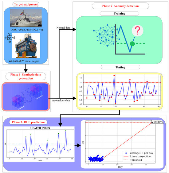
Figure 1. Block diagram of the general idea of the approach.

3.1. Target Equipment

The PdM approach is specifically designed for the ARC “20 de Julio” (PZE-46) (manufactured by Colombian Navy, Cartagena, Colombia), an offshore patrol vessel of the Colombian Navy; this vessel is shown in Figure 2. Within this vessel, the critical system selected for implementation is the main propulsion system. This system is vital for the operational capability of the vessel, and its reliability is crucial for mission success.

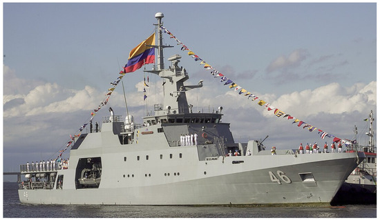
Figure 2. ARC “20 de Julio” (PZE-46).

Propulsion System

The propulsion system is powered by a Wärtsilä 6L26 diesel engine (manufactured by Wärtsilä Italia S.p.A., Trieste, Italy), which converts the chemical energy of fuel into mechanical power to drive the propeller and generate the thrust required for the vessel’s navigation on missions. This engine, which represents the core component of the ship’s propulsion system, is shown in Figure 3.

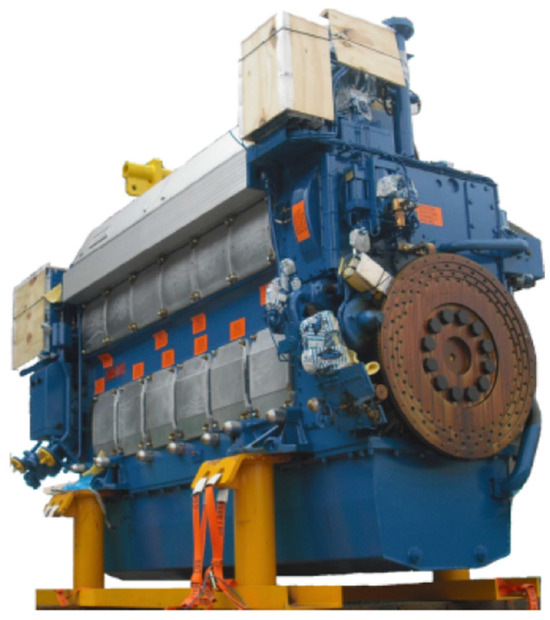
Figure 3. Wärtsilä 6L26 diesel engine.

The diesel engine is structured into several subsystems—namely cooling, fuel, lubrication, and exhaust gas—each characterized by a set of interrelated variables. These monitoring variables provide a comprehensive representation of the engine’s operating condition and are summarized in Table 2.

Table 2. Subsystems and variables of the targeted equipment.

Subsystem	Variable	Min	Nominal	Max
Cooling	HT inlet pressure (PT401) [bar]	1.6	4,2	5
	HT inlet temperature (TE401) [°C]	61	88	-
	LT inlet pressure (PT471) [bar]	1.6	3,6	5
	Charge air temperature (TE600) [°C]	-	60	-
	Turbo inlet air temperature (TE600) [°C]	-	45	45
Fuel	Engine F.O. inlet pressure (PT101) [bar]	6	7	7.5
	Engine F.O. inlet temperature (TE101) [°C]	30	45	50
Lubrication	Engine speed [RPM]	650	998	1000
	Engine L.O. inlet temperature (TE201) [°C]	-	68	75
	Engine L.O. outlet temperature (TE202) [°C]	-	78	-
	Turbo L.O. outlet temperature (TE272) [°C]	-	105	105
	Oil filter differential pressure (PDT243) [bar]	-	0,8	-
	Turbo L.O. inlet pressure (PT271) [bar]	-	4.5	4.5
	Fresh water inlet temperature (XX001) [°C]	-	-	-
	Fresh water outlet temperature (XX002) [°C]	-	38	38
	Fresh water temperature difference (XX002–XX001) [°C]	-	12	12
Exhaust gas	Exhaust gas turbo inlet temperature (TE511) [°C]	-	600	600
	Exhaust gas turbo outlet temperature (TE517) [°C]	-	495	500
	Maximum cylinder temperature (TE5011A) [°C]	-	400	490

3.2. Synthetic Data Generation

To ensure the development and validation of the proposed approach, it is essential to work with data that adequately represent both normal operating conditions and possible anomalous behaviors of the system. Since the available measurements are limited and do not cover the full range of operational scenarios, synthetic data are generated within the specified ranges using suitable techniques to realistically capture the dynamics of the system’s variables. To achieve this, different methods for synthetic data generation are tested and compared: TBN is used to generate data without using seeds, while TVAE, CTGAN, and GC are applied to generate data based on initial seeds. The objective is to obtain representative data for model training under normal conditions as well as anomalous data for testing and validation in later stages.

3.2.1. Synthetic Data Generation Without Seeds

The TBN approach enables the modeling of the stochastic behavior of system variables through parent–child relationships between nodes. In this implementation, each node represents a system variable, such as pressure, temperature, or speed. A node can have dependencies on other nodes—referred to as parents—whose outputs directly influence its behavior. This structure allows for the simulation of causal relationships among subsystem variables.

The dynamics of each variable are modeled based on its respective operating range, which is discretized into 10 states. The first five (5) states correspond to normal operating conditions, while the remaining five (5) represent deviations, failures, or anomalous behaviors. This discretization allowed for the generation of data that simulates both normal conditions—defined as those within the operational range—and abnormal conditions, associated with values outside of that range.

Transitions between these states are governed by a probability transition matrix, which defines the likelihood of a variable moving from one state to another at the next time step. This matrix is adjusted to favor specific transition paths according to the expected behavior of the system, whether under normal or abnormal conditions.

Based on this strategy, synthetic data is generated using TBN, capable of simulating both normal and anomalous behaviors.

From this point, the use of the different models in each section of this manuscript is going to be exemplified using specifically the fuel subsystem or its variables because of space limitations. Figure 4 shows the synthetic data generated for the fuel subsystem using TBN.

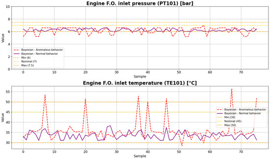
Figure 4. Synthetic data of the fuel subsystem generated using TBN.

3.2.2. Synthetic Data Generation with Seeds

One of the inputs provided by the Colombian Navy for this approach consisted of hourly data from variables of interest collected during different missions. These are referred to as the original data. The dataset is limited in size, containing only 76 data points per variable. These are concatenated into a single time series for each variable in order to capture their dynamics and use them as seeds for synthetic data generation. This strategy aimed to expand both the training and testing datasets.

Since the original data is not labeled as normal or anomalous, a rule-based classification criterion is adopted using predefined value ranges. Specifically, any observation in which a variable exceeded its range thresholds is considered anomalous.

Given that the data received from the Navy already included values outside of acceptable ranges, a preprocessing step is applied to generate seeds representing normal behavior. Values exceeding defined limits are truncated to the nearest threshold. Meanwhile, the original, unmodified data is used as a seed for generating anomalous data. Figure 5 shows both the original and truncated data for PT101.

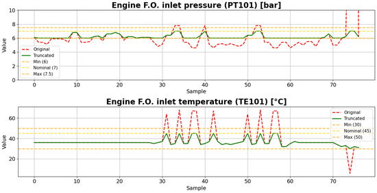
Figure 5. Original data of the fuel subsystem provided by the Colombian Navy and its truncated version.

Subsequently, three synthetic data generation methods are compared: GC, TVAE, and CTGAN. The evaluation is conducted using metrics designed to assess the fidelity of synthetic datasets, focusing both on the overall distribution of individual variables and on the relationships among them. The metric known as Column Shapes evaluates whether each variable in the synthetic data preserves the same distributional characteristics as in the real data, ensuring similarity in aspects such as mean, variance, and overall shape. Complementarily, the Column Pair Trends score measures how well the synthetic data captures the dependencies between pairs of variables by comparing their correlations, thus reflecting whether the generated data reproduces the patterns of association present in the real dataset [19]. The results of the comparison are shown in Table 3.

Table 3. Comparison of the results of the different synthetic data generation techniques with seeds.

Model	Column Shapes Score (%)	Column Pair Trends Score (%)	Overall Score (%)
GC	66.37	92.94	79.65
TVAE	78.95	91.14	85.05
CTGAN	55.87	87.31	71.59

Of these techniques, the one that showed the best performance is the TVAE. When compared to the previous approach based on TBN, the TVAE demonstrated a greater ability to replicate both the individual distributions and the relationships between variables, as can be seen in Table 4. Figure 6 shows synthetic data generated using the TVAE approach.

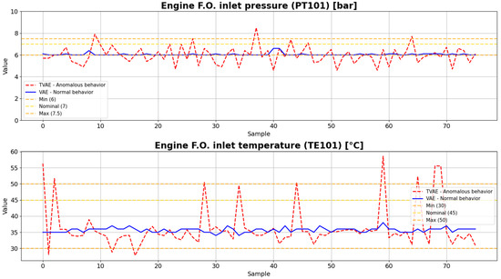
Figure 6. Synthetic data of the fuel subsystem generated using TVAE.

Table 4. Comparison of the results of the different synthetic data generation techniques, TBN–TVAE.

Model	Column Shapes Score (%)	Column Pair Trends Score (%)	Overall Score (%)
TBN	60.67	84.46	72.57
TVAE	78.68	91.43	85.05

Table 4. Comparison of the results of the different synthetic data generation techniques, TBN–TVAE.

Model	Column Shapes Score (%)	Column Pair Trends Score (%)	Overall Score (%)
TBN	60.67	84.46	72.57
TVAE	78.68	91.43	85.05

3.3. Anomaly Detection

After generating and validating the synthetic data, the training and testing of various state-of-the-art anomaly detection models are carried out. To compare the performance of each technique, the silhouette score is calculated for each trained model when presented with anomalous data. The silhouette score measures how well each sample is separated from other clusters or groups, with higher values indicating that anomalies are more clearly distinguishable from normal data. The silhouette score for a singular data point is calculated using Equation (1).

$$\mathrm{s}(\mathrm{i})={\displaystyle \frac{\mathrm{b}\left(\mathrm{i}\right)-\mathrm{a}\left(\mathrm{i}\right)}{\mathrm{m}\mathrm{a}\mathrm{x}(\mathrm{a}\left(\mathrm{i}\right),\mathrm{b}(\mathrm{i}\left)\right)}}$$

(1)

where

• $\mathrm{a}\left(\mathrm{i}\right)$: Average distance from point $\mathrm{i}$ to all other points in the same group.
• $\mathrm{b}\left(\mathrm{i}\right)$: Average distance from point $\mathrm{i}$ to the nearest other group.

The global silhouette score is the average of the singular scores for each data point [20]. This metric is used because, although we have labeled which data points are anomalous—based on whether they fall outside predefined ranges—we cannot assess model performance solely by counting the number of points detected outside these ranges. This is because the models may also identify anomalous dynamics that, while within the expected ranges, deviate from the normal temporal behavior of the data. If performance evaluation is based only on whether a point falls outside the range, a conditional statement would suffice, and the ability of the model to capture more subtle anomalies would be ignored. Such subtle anomalies can occur in real systems, like the target equipment.

The green points shown in the figures are used purely for illustrative purposes. They indicate cases where the anomalous behavior of a variable coincides with values outside the expected operational range of the synthetic anomalous data. This visualization is intended to help the reader identify some of the more obvious deviations, but it does not represent the sole basis of the anomaly detection method, which evaluates the dynamic behavior of the variables over time rather than relying on a range-based threshold.

3.3.1. One-Class SVM

Synthetic data representing normal behavior is used to train One-Class SVM models. Separate models are trained for each monitored variable, exploring different kernel functions, including linear, polynomial (POLY), radial basis function (RBF), and sigmoid. This approach allowed for evaluating the suitability of each kernel in capturing the normal patterns of the variables, providing a basis for detecting deviations indicative of anomalies.

Examples of anomaly detection using One-class SVM model trained on normal data of the fuel subsystem variable PT101 are shown in Figure 7. Table 5 shows the Silhouette scores of each SVM trained and tested on anomalous data. The scores of each example are marked in blue in each table for every tested model.

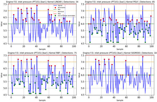
Figure 7. Anomaly detection testing on PT101 with one-class SVM.

Table 5. Silhouette scores of each SVM trained and tested on anomalous data.

Subsystem	Variable	LINEAR	POLY	RBF	SIGMOID
Cooling	HT inlet pressure (PT401) [bar]	0.25	0.48	0.09	−0.05
	HT inlet temperature (TE401) [°C]	0.67	0.67	0.7	0.67
	LT inlet pressure (PT471) [bar]	0.47	0.48	0.28	0.44
	Charge air temperature (TE600) [°C]	0.68	0.62	0.05	0.55
	Turbo inlet air temperature (TE600) [°C]	0.53	0.54	0.39	0.34
Fuel	Engine F.O. inlet pressure (PT101) [bar]	0.07	0.46	0.54	0.46
	Engine F.O. inlet temperature (TE101) [°C]	0.97	0.49	0.1	0.23
Lubrication	Engine speed [RPM]	0.18	0.51	0.46	0.51
	Engine L.O. inlet temperature (TE201) [°C]	0.28	0.03	0.06	0.01
	Engine L.O. outlet temperature (TE202) [°C]	0.1	0.76	0.64	0.77
	Turbo L.O. outlet temperature (TE272) [°C]	0.12	0.46	0.3	−0.03
	Oil filter differential pressure (PDT243) [bar]	0.57	0.59	0.11	0.08
	Turbo L.O. inlet pressure (PT271) [bar]	0.52	0.52	0.09	0.51
	Fresh water inlet temperature (XX001) [°C]	0.86	0.85	0.76	0.82
	Fresh water outlet temperature (XX002) [°C]	0.43	0.56	0.13	0.49
	Fresh water temperature difference (XX002–XX001) [°C]	0.74	0.08	0.71	0.72
Exhaust gas	Exhaust gas turbo inlet temperature (TE511) [°C]	0.24	−0.29	0.26	−0.11
	Exhaust gas turbo outlet temperature (TE517) [°C]	−0.01	0.86	0.43	−0.12
	Maximum cylinder temperature (TE5011A) [°C]	0.5	0.02	0.39	−0.14

3.3.2. Autoencoders

An autoencoder is a type of neural network designed to learn a compressed representation of input data through an encoder–decoder structure. The encoder maps the input to a lower-dimensional latent space, while the decoder reconstructs the input from this representation. In this work, autoencoders are trained on normal operating data for each variable, and the reconstruction error is monitored; deviations from expected reconstruction indicate anomalies, allowing the detection of anomalous behavior in the system.

For each variable within the subsystems, a grid search is performed to determine the activation function that most effectively minimizes reconstruction error during the training of the corresponding autoencoder models. The threshold considered for anomaly detection corresponds to the maximum reconstruction error observed during training with normal behavior data. Figure 8 shows anomaly detection examples on anomalous samples of PT101 using the respective trained autoencoders, and Table 6 shows the silhouette score for each variable.

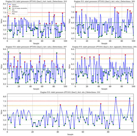
Figure 8. Anomaly detection testing on PT101 with autoencoders.

Table 6. Silhouette scores of each autoencoder trained and tested on anomalous data.

Subystem	Variable	Elu	Relu	Selu	Sigmoid	Tanh
Cooling	HT inlet pressure (PT401) [bar]	0.48	0.54	0.46	0.46	0.46
	HT inlet temperature (TE401) [°C]	0.87	0.96	0.87	0.96	0.86
	LT inlet pressure (PT471) [bar]	0.47	0.43	0.44	0.48	0.43
	Charge air temperature (TE600) [°C]	0.6	0.57	0.61	0.66	0.66
	Turbo inlet air temperature (TE600) [°C]	0.52	0.53	0.54	0.52	0.53
Fuel	Engine F.O. inlet pressure (PT101) [bar]	0.57	0.44	0.22	0.44	0.34
	Engine F.O. inlet temperature (TE101) [°C]	0.97	0.97	0.97	0.97	0.97
Lubrication	Engine speed [RPM]	0.55	0.57	0.57	0.56	0.57
	Engine L.O. inlet temperature (TE201) [°C]	0.59	0.44	0.58	0.16	0.47
	Engine L.O. outlet temperature (TE202) [°C]	0.94	0.95	0.94	0.95	0.93
	Turbo L.O. outlet temperature (TE272) [°C]	0.26	0.48	0.12	0.34	0.09
	Oil filter differential pressure (PDT243) [bar]	0.53	0.79	0.52	0.71	0.76
	Turbo L.O. inlet pressure (PT271) [bar]	0.15	0.13	0.19	0.14	0.2
	Fresh water inlet temperature (XX001) [°C]	0.8	0.82	0.81	0.79	0.8
	Fresh water outlet temperature (XX002) [°C]	0.44	0.43	0.43	0.45	0.44
	Fresh water temperature difference (XX002–XX001) [°C]	0.77	0.82	0.77	0.76	0.77
Exhaust gas	Exhaust gas turbo inlet temperature (TE511) [°C]	0.32	−0.03	−0.2	0.39	0.41
	Exhaust gas turbo outlet temperature (TE517) [°C]	0.41	0.64	0.09	0.45	0.26
	Maximum cylinder temperature (TE5011A) [°C]	0.48	−0.07	−0.02	0.54	0.13

3.3.3. LSTM Autoencoders

An LSTM autoencoder is a neural network architecture specifically designed to capture temporal dependencies in sequential data. Similarly to traditional autoencoders, it consists of an encoder that compresses input sequences into a lower-dimensional latent space and a decoder that reconstructs the original sequences from this representation. In this work, an LSTM autoencoder is trained independently for each variable on normal operating sequences, and reconstruction error is monitored to detect anomalies.

Before training the models, the raw time series are preprocessed through two key steps, sequence generation and feature scaling. Since LSTM models require sequential inputs of fixed length, each continuous signal is segmented into overlapping windows, or sequences, of length T. For example, given a time series of N samples, a sliding window approach is applied to generate multiple sequences of size T, where each sequence preserves the temporal order of the original data. This procedure allows the network to learn short-term and long-term temporal dependencies rather than treating each observation as independent. The choice of sequence length is fixed across all variables to ensure consistency in training and testing. In our case T = 30. In addition, all signals are normalized prior to sequence construction using Min-Max scaling to the range [0, 1]. This scaling process prevents variables with larger numerical ranges from dominating the loss function and improves the stability of the training process. The model architecture includes two LSTM layers with 128 hidden units each and tanh activation, combined with Dropout layers to prevent overfitting. The encoder compresses the input sequence into a latent vector, and the decoder reconstructs the sequence using a RepeatVector layer followed by a second LSTM layer and a Time-Distributed Dense output layer. These hyperparameters—including the number of hidden units, activation function, dropout rate, and sequence length—are fixed and applied uniformly to all variables.

For each variable, the anomaly detection threshold corresponds to the maximum reconstruction MAE observed during training with normal sequences. This choice is made considering that different error metrics can be used, such as the Mean Squared Error (MSE) or the MAE. While MSE penalizes larger deviations more heavily due to the squaring operation, it tends to be overly sensitive to outliers, which may result in thresholds that do not adequately represent the general behavior of the system. On the other hand, MAE provides a more robust and interpretable measure, as it reflects the average magnitude of the reconstruction errors without disproportionately amplifying occasional extreme values. By adopting the maximum MAE from training, the threshold ensures that all reconstruction patterns observed under normal operating conditions are correctly recognized as non-anomalous, while values exceeding this bound can be reliably considered indicative of abnormal behavior. This criterion follows the insights from previous related works, which recommend data-driven thresholding strategies based on reconstruction error distributions to improve robustness in anomaly detection tasks. Figure 9 illustrates an example of anomaly detection on a sample of PT101 and its reconstruction MAE, and Table 7 reports the silhouette score for each variable.

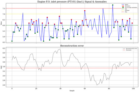
Figure 9. Anomaly detection testing on PT101 with LSTM autoencoder.

Table 7. Silhouette scores of each LTSM autoencoder trained and tested on anomalous data.

Subsystem	Variable	Silhouette Score
Cooling	HT inlet pressure (PT401) [bar]	0.69
	HT inlet temperature (TE401) [°C]	0.84
	LT inlet pressure (PT471) [bar]	0.57
	Charge air temperature (TE600) [°C]	0.65
	Turbo inlet air temperature (TE600) [°C]	0.67
Fuel	Engine F.O. inlet pressure (PT101) [bar]	0.61
	Engine F.O. inlet temperature (TE101) [°C]	0.88
Lubrication	Engine speed [RPM]	0.75
	Engine L.O. inlet temperature (TE201) [°C]	0.84
	Engine L.O. outlet temperature (TE202) [°C]	0.82
	Turbo L.O. outlet temperature (TE272) [°C]	0.64
	Oil filter differential pressure (PDT243) [bar]	0.73
	Turbo L.O. inlet pressure (PT271) [bar]	0.57
	Fresh water inlet temperature (XX001) [°C]	0.56
	Fresh water outlet temperature (XX002) [°C]	0.66
	Fresh water temperature difference (XX002–XX001) [°C]	0.57
Exhaust gas	Exhaust gas turbo inlet temperature (TE511) [°C]	0.56
	Exhaust gas turbo outlet temperature (TE517) [°C]	0.69
	Maximum cylinder temperature (TE5011A) [°C]	0.57

3.3.4. Multivariate LSTM Autoencoders

A multivariate LSTM autoencoder is an extension of the standard LSTM autoencoder designed to process multiple time series variables simultaneously. While a univariate model focuses only on the temporal dynamics of a single variable, the multivariate approach allows the network to learn not only temporal dependencies within each signal but also cross-correlations between different variables. This is particularly advantageous in complex systems where anomalies often manifest through interactions among several signals rather than in isolation. By modeling multiple variables together, a multivariate LSTM autoencoder can better capture the joint behavior of the system, leading to more robust reconstructions and improved anomaly detection performance.

Before training, the raw time series are preprocessed following the same procedure described for the univariate case, all signals are normalized using Min-Max scaling to the range [0, 1], and then segmented into overlapping sequences of fixed length T using a sliding window approach. This ensured that the models received inputs with consistent numerical ranges and preserved the temporal structure of the data.

For the multivariate case, a separate LSTM autoencoder is trained for each subsystem, grouping together its corresponding variables. Unlike the univariate approach, where a fixed network configuration is used, here a grid search is performed for each subsystem model to optimize its performance. The search varied the activation function, the number of hidden units in the LSTM layers, and the dropout rate. The best configuration for each subsystem is selected according to the silhouette score, ensuring that the learned latent representations maximize the separability between normal and anomalous sequences.

The definition of the anomaly detection threshold also follows the same criterion applied in the univariate LSTM autoencoders, that is, the maximum reconstruction MAE observed during training with normal sequences. By keeping this consistent strategy across both univariate and multivariate cases, the models ensure methodological coherence and comparability, while retaining the robustness of MAE against outliers and its interpretability for anomaly detection.

This procedure allowed each subsystem model to adapt its architecture to the specific dynamics of its variables. Since this technique yielded the best overall performance, it is directly implemented in the user interface developed for the Colombian Navy. Consequently, the figure that illustrates anomaly detection for the fuel subsystem (Figure 10) is shown in a different format, reflecting its integration into the final application. Table 8 summarizes the results for all subsystems.

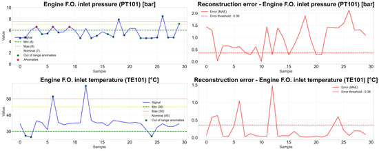
Figure 10. Anomaly detection testing on the fuel subsystem variables with multivariate LSTM autoencoder.

Table 8. Silhouette scores of each multivariate LSTM autoencoder trained and tested on anomalous data.

Subsystem	Hidden Units	Dropout	Activation	Silhouette Score
Cooling	64	0.3	tanh	0.71
Fuel	128	0.2	tanh	0.77
Lubrication	64	0.2	tanh	0.75
Exhaust gas	64	0.3	relu	0.74

After evaluating multiple anomaly detection models, the multivariate LSTM autoencoder is selected as the optimal model for the target subsystems. This choice is based on two main reasons. First, the multivariate LSTM autoencoder is capable of capturing both the temporal dynamics of each variable—similar to a univariate LSTM autoencoder—and the inter-variable relationships and correlations within the specific subsystem used for training. This allows the model to account for complex interactions between variables while preserving the temporal evolution of each signal. Second, although the silhouette scores of individual conventional autoencoders are occasionally higher for specific variables, the multivariate LSTM models consistently achieved higher overall scores across all variables. This consistent performance demonstrates the robustness of the multivariate LSTM autoencoder relative to other models. The comparative results can be verified through inspection of the tables of tested models (Table 5, Table 6, Table 7 and Table 8), which show that this model provides a balanced and generally superior performance across the full set of variables.

3.4. RUL Prediction

To estimate the RUL of each subsystem, we defined an observation period of one day. For each day, all subsystem variables are collected and passed through the anomaly detection process of the corresponding multivariate LSTM autoencoder in order to compute their reconstruction MAE. The MAE of all variables within the subsystem is computed to obtain a daily HI as seen in (2), and this procedure is repeated for every subsequent day. In this work, the daily HI is computed as the arithmetic average of the MAE values of all subsystem variables. This choice assumes that all variables contribute equally to the overall degradation behavior of the subsystem, avoiding the introduction of additional assumptions or biases regarding the relative importance of each signal. The unweighted average also ensures a transparent and consistent aggregation across subsystems, which is particularly suitable at this prototyping stage, where no validated criteria are available to objectively define variable-specific weights.

$$\mathrm{H}\mathrm{I}=\mathrm{a}\mathrm{v}\mathrm{g}({\mathrm{h}\mathrm{i}}_{1,\mathrm{d}},{\mathrm{h}\mathrm{i}}_{2,\mathrm{d}},\dots ,{\mathrm{h}\mathrm{i}}_{\mathrm{n},\mathrm{d}})$$

(2)

where

• $\mathrm{d}$: Observation day.
• $\mathrm{H}\mathrm{I}$: Health index of the subsystem on day $\mathrm{d}$.
• $\mathrm{n}$: Number of variables in the subsystem.
• ${\mathrm{h}\mathrm{i}}_{\mathrm{i},\mathrm{d}}$: Health index of variable $\mathrm{i}$ on day $\mathrm{d}$ calculated as the average MAE of that day for that variable.

Once more than 30 days of HI values are available, the most recent 30-day window is used to fit the linear regression model in (3), ensuring that the regression captures the monthly trend leading up to the day under study.

$$\mathrm{H}\mathrm{I}=\mathrm{a}·\mathrm{d}+\mathrm{b}$$

(3)

where

• $\mathrm{b}$: Intercept of the regression line.
• $\mathrm{a}$: Slope of the regression line (degradation trend of the subsystem).

The predicted failure day is calculated with (4) as the point in the future where this regression line intersects the anomaly threshold defined during training of the respective multivariate LSTM autoencoder. The RUL is then computed with (5) as the difference between the estimated intersection day and the current observation day.

$${\mathrm{d}}_{\mathrm{f}\mathrm{a}\mathrm{i}\mathrm{l}}={\displaystyle \frac{\mathrm{t}\mathrm{h}-\mathrm{b}}{\mathrm{a}}}$$

(4)

$$\mathrm{R}\mathrm{U}\mathrm{L}={\mathrm{d}}_{\mathrm{f}\mathrm{a}\mathrm{i}\mathrm{l}}-{\mathrm{d}}_{\mathrm{c}\mathrm{u}\mathrm{r}\mathrm{r}\mathrm{e}\mathrm{n}\mathrm{t}}$$

(5)

where

• $\mathrm{t}\mathrm{h}$: Anomaly threshold defined during training of the multivariate LSTM autoencoder.
• ${\mathrm{d}}_{\mathrm{f}\mathrm{a}\mathrm{i}\mathrm{l}}$: Estimated intersection day when the HI trend reaches the threshold.
• ${\mathrm{d}}_{\mathrm{c}\mathrm{u}\mathrm{r}\mathrm{r}\mathrm{e}\mathrm{n}\mathrm{t}}$: Current observation day.
• $\mathrm{R}\mathrm{U}\mathrm{L}$: estimated remaining useful life of the subsystem (in days).

Figure 11 illustrates the initial stage of the proposed process. After 32 pre-charged days, included for simulation purposes since at least 30 observations are required to capture the monthly trend, nine (9) additional days of normal behavior are simulated (green circled HI). Each blue dot represents the HI of a given day, with the HI on day 40 reaching 0.09. Because the behavior observed up to this point remains below the subsystem threshold, the red trend line never intersects it. Consequently, the interpretation is that the subsystem is in acceptable condition, as reported in the developed interface shown in Figure 12. The interface also provides information on the individual variables of the subsystem, allowing the user to decide which variable should be prioritized when scheduling maintenance.

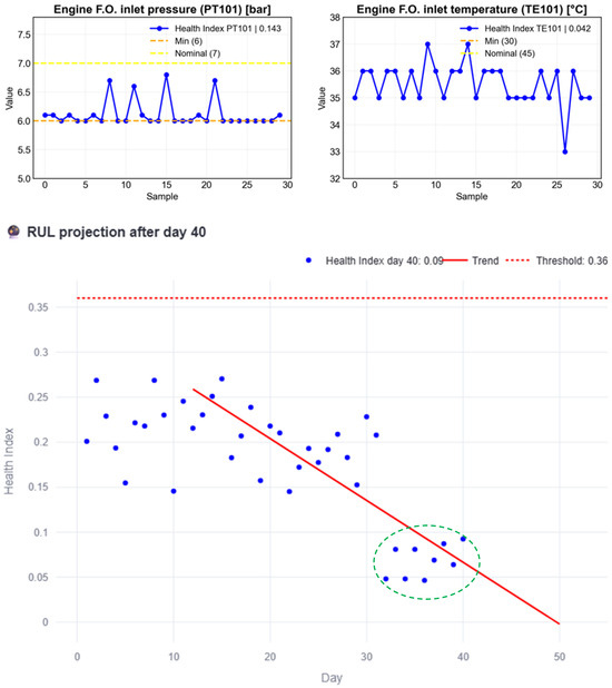
Figure 11. RUL estimation process example with normal behavior data until day 33.

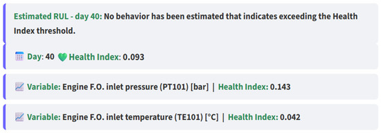
Figure 12. Interface report of the subsystem behavior up to day 40.

At this stage, anomalous data is introduced after day 40 into the simulations to analyze its impact on the RUL estimation. Figure 13 illustrates this case; anomalous data is present from day 41 to 45 as evidenced by each HI (green circled HI) surpassing the threshold. Based on the data up to day 45, the line trend intersects the threshold on day 52, yielding a RUL of 7 days; these insights are reported in the interface, as shown in Figure 14, which also shows how the RUL started to decrease over time.

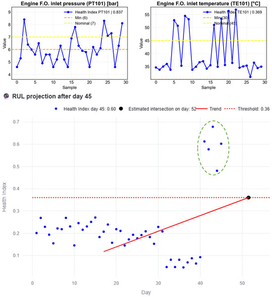
Figure 13. RUL estimation process example with anomalous data from days 41 to 45.

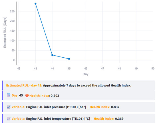
Figure 14. RUL vs. day graph and report up to day 45.

At this stage, maintenance should be scheduled before the estimated failure day to address the problem, prioritizing the components related to PT101, since its HI is higher than that of TE101. But what happens if no maintenance action is taken? Figure 15 presents a simulation in which anomalous data continues until day 48 (green circled HI). In this scenario, the anomalous behavior causes the RUL to decrease to the point where the intersection shifts beyond the current day, clearly indicating that maintenance should have been performed earlier.

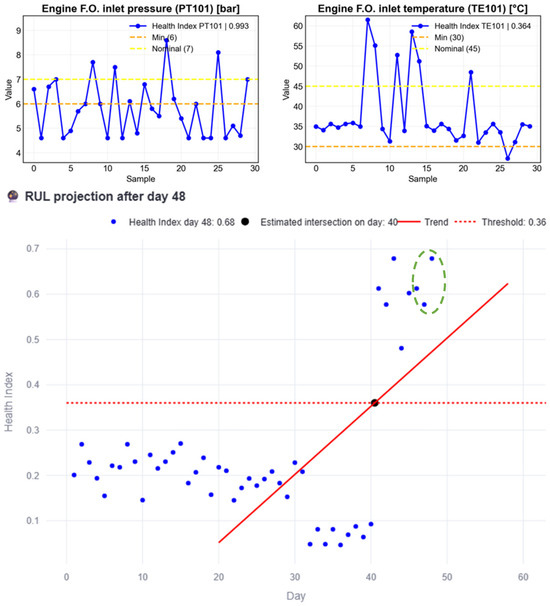
Figure 15. RUL estimation process example when there is no maintenance action after the failure day.

Figure 16 illustrates the case where the subsystem is repaired, restoring its normal behavior. The RUL begins to increase over the following 15 simulated days (green circled HI), until day 61, when no intersection exists, evidence of restored normality.

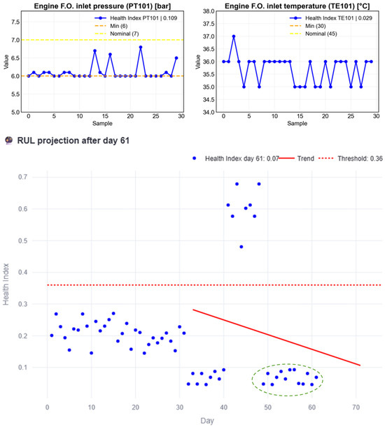
Figure 16. RUL estimation process example after maintenance is done.

Figure 17 further confirms that the RUL continues to decrease in the absence of maintenance. It can also be observed that the variable with the highest HI is PT101, with a value of 0.993, compared to the HI of TE101, which reaches 0.364. Moreover, the interface indicates that a maintenance action should have been planned in advance, specifically eight (8) days earlier, as that is the point when the anomalous behavior began.

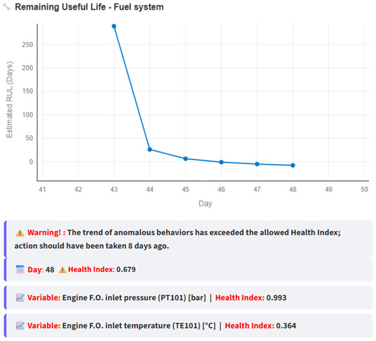
Figure 17. RUL vs. day graph and conclusions based on the RUL when maintenance is not done.

Figure 18 demonstrates the increase in RUL following repairs. Notably, no RUL is plotted since day 59, indicating the day when the intersection ceased to exist.

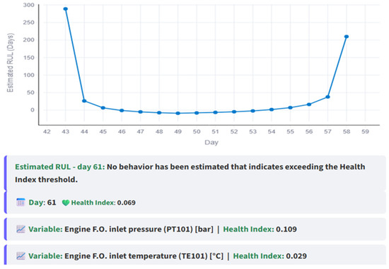
Figure 18. RUL vs. day graph and conclusions based on the RUL after maintenance is done.

In summary, the proposed approach effectively predicts the RUL by capturing the impact of anomalies in subsystem behavior. When anomalies occur, the model estimates shorter RUL values, signaling proximity to failure due to variable degradation. At the same time, the system monitors the HI of each variable, enabling identification of the most critical components through higher MAE values. This information assists personnel in prioritizing maintenance actions. Additionally, the RUL-versus-day plots provide a dynamic view of subsystem condition, showing how degradation or interventions affect the RUL, thereby supporting informed decision-making and proactive maintenance planning for Navy operations.

Finally, Figure 19 revisits the block diagram of the proposed framework, now enriched with the specific technologies used in its implementation: TVAE for synthetic data generation and multivariate LSTM autoencoders for anomaly detection, which together enable computation of the MAE and subsequent RUL prediction.

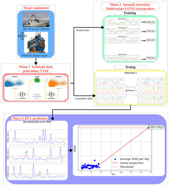
Figure 19. Block diagram of the proposed approach with the specific technologies used.

4. Experimental Results

In order to perform more robust tests, we used a new dataset provided by the Colombian Navy, acquired during operational missions. This dataset contains up to 40,000 data points per variable with a sampling frequency of 40 s. Unlike the seed dataset mentioned previously—which consisted of only 76 observations at a rate of one per hour—this new dataset also includes additional variables and subsystems, which are detailed in Table 9.

Table 9. Subsystems and variables from the new data.

Subsystem	Variable	Min	Nominal	Max
Fuel	Engine F.O. inlet pressure (PT101) [bar]	6	7	7.5
	Engine F.O. inlet temperature (TE101) [°C]	30	45	50
Lubrication	Turbo L.O. outlet temperature (TE272) [°C]	-	105	105
	Engine L.O. inlet pressure (PT201) [bar]	3	5,1	5
	Engine L.O. inlet temperature (TE201) [°C]	-	68	75
	Oil filter differential pressure (PDT243) [bar]	-	0.8	-
	Engine L.O. outlet temperature (TE202) [°C]	-	78	-
	Turbo L.O. inlet pressure (PT271) [bar]	-	4,5	4.5
Cooling	HT inlet temperature (TE401) [°C]	61	88	-
	HT outlet temperature (TE402) [°C]	-	93	96
	LT inlet temperature (TE471) [°C]	25	46	38
Exhaust gases	Maximum cylinder temperature (TE5011A) [°C]	-	400	490
	Maximum cylinder temperature (TE5021A) [°C]	-	400	490
	Maximum cylinder temperature (TE5031A) [°C]	-	400	490
	Maximum cylinder temperature (TE5041A) [°C]	-	400	490
	Maximum cylinder temperature (TE5051A) [°C]	-	400	490
	Maximum cylinder temperature (TE5061A) [°C]	-	400	490
Bearing	Main bearing 00 temp (TE700)	-	110	-
	Main bearing 01 temp (TE701)	-	110	-
	Main bearing 02 temp (TE702)	-	110	-
	Main bearing 03 temp (TE703)	-	110	-
	Main bearing 04 temp (TE704)	-	110	-
	Main bearing 05 temp (TE705)	-	110	-
Charge air	CA press, engine inlet (PT601)	-	3.4	-
	CA temp, engine inlet (TE601)	25	65	-
	Air temp, TC inlet (TE600)	-	45	-
Others	Starting air pressure, engine inlet (PT301)	7	-	-
	Control air pressure (PT311)	15	-	-

The objective of this section is to replicate the proposed approach with these new variables and data in order to demonstrate its capability to work regardless of the dataset used.

4.1. Data Preparation and Synthetic Data Generation

An example of the raw signals provided for analysis is shown in Figure 20, which depicts the new signals from the fuel subsystem. As can be seen, the raw data contains missing points that appear as visible gaps in the signals.

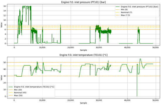
Figure 20. Fuel subsystem variables from the raw new data.

Figure 21 presents the processed version of these signals, where the missing points are addressed by reindexing the time series to remove such gaps and ensure a continuous sequence of samples. The purple segments in Figure 21 correspond to the interval [29,000, 34,000], which is selected as the seed to generate synthetic data with TVAE, since visual inspection suggests that this interval reflects a particular system dynamic associated with a ship mission operation.

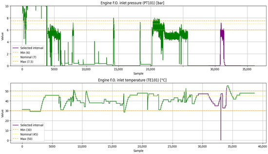
Figure 21. Fuel subsystem variables from the processed new data.

The synthetic normal data generated using TVAE is shown in Figure 22, while the anomalous data generated is presented in Figure 23. Finally, Table 10 reports the performance metrics of the data generation process with these new seeds.

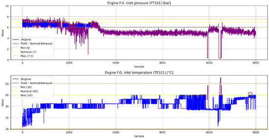
Figure 22. Fuel subsystem normal synthetic data generated using TVAE.

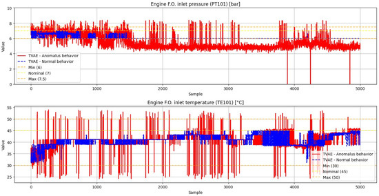
Figure 23. Fuel subsystem anomalous synthetic data generated using TVAE.

Table 10. Performance metrics of the newly generated data.

Model	Column Shapes Score (%)	Column Pair Trends Score (%)	Overall Score (%)
TVAE	91.05	95.66	93.36

4.2. Anomaly Detection Results

The generated normal-behavior data is used to train new multivariate LSTM autoencoders, enabling anomaly detection and, consequently, RUL prediction based on this new dataset. Figure 24 illustrates examples of anomaly detection in the fuel subsystem.

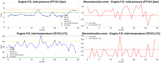
Figure 24. Anomaly detection testing on the new fuel system data.

To statistically validate whether the reconstruction MAE is significantly higher under anomalous conditions compared to normal conditions when using the trained models, we conducted hypothesis testing at the subsystem level. To assess whether anomalous sequences yield significantly higher reconstruction MAE compared to normal sequences, a statistical experiment based on mean comparison is designed.

For each subsystem, two groups of data are considered: 50 generated sequences of normal operation and 50 generated sequences of anomalous operation. Each sequence corresponds to a window of 30 consecutive time steps, and each sequence is evaluated with the new trained models.

The hypotheses to conduct the tests for each subsystem are defined in (6):

$$\left\{\begin{array}{c}{\mathrm{H}}_0:{\mathsf{\mu }}_{\mathrm{A}}={\mathsf{\mu }}_{\mathrm{N}}\\ {\mathrm{H}}_1:{\mathsf{\mu }}_{\mathrm{A}}>{\mathsf{\mu }}_{\mathrm{N}}\end{array}\right.$$

(6)

Null hypothesis ${(\mathrm{H}}_0)$: The mean reconstruction MAE of normal sequences ${(\mathsf{\mu }}_{\mathrm{N}})$ is equal to that of anomalous sequences.

Alternative hypothesis ${(\mathrm{H}}_1$): The mean reconstruction MAE of anomalous sequences ${(\mathsf{\mu }}_{\mathrm{A}})$ is greater than that of normal sequences.

Because we cannot assume equal population variances, Welch’s t-test is employed. Unlike Student’s t-test, this approach does not require homogeneity of variances and thus provides a more reliable comparison between two independent samples [21].

The corresponding test statistic is defined in Equation (7).

$$\mathrm{t}={\displaystyle \frac{{\overline{\mathrm{x}}}_1-{\overline{\mathrm{x}}}_2}{\sqrt{\frac{{\mathrm{s}}_1^2}{\mathrm{n}}+\frac{{\mathrm{s}}_2^2}{\mathrm{n}}}}}$$

(7)

where

• ${\overline{\mathrm{x}}}_1 \mathrm{and} {\overline{\mathrm{x}}}_2$ are the normal and anomalous sample reconstruction MAE means, respectively.
• ${\mathrm{s}}_1^2 \mathrm{and} {\mathrm{s}}_2^2$ are the normal and anomalous sample variances, respectively.
• $\mathrm{n}$ is the normal and anomalous sequences sample size (50).

The adjusted degrees of freedom $\left(\mathrm{v}\right)$ are calculated using the Welch–Satterthwaite equation in (8):

$$\mathrm{v}={\displaystyle \frac{{\left(\frac{{\mathrm{s}}_1^2}{\mathrm{n}}+\frac{{\mathrm{s}}_2^2}{\mathrm{n}}\right)}^2}{\frac{{\left(\frac{{\mathrm{s}}_1^2}{\mathrm{n}}\right)}^2}{\mathrm{n}-1}+\frac{{\left(\frac{{\mathrm{s}}_2^2}{\mathrm{n}}\right)}^2}{\mathrm{n}-1}}}$$

(8)

The assumptions of Welch’s t-test are that observations within each group are independent and that each group approximately follows a normal distribution. In this study, each group consisted of 50 samples. According to the Central Limit Theorem, when the sample size is sufficiently large—commonly considered greater than 50 observations—the sampling distribution of the mean tends to approximate a normal distribution, regardless of whether the underlying data are normally distributed. This supports the validity of applying Welch’s t-test even if the individual reconstruction errors are not strictly normal.

Regarding independence, each sequence is synthetically generated as a separate realization for the experiment, rather than being derived by segmenting a single long time series into shorter subsequences. This design choice ensures that the sequences do not share temporal overlap or mutual dependence, allowing them to be treated as independent observations and thereby satisfying the independence assumption required by the test. The results of the tests are shown in Table 11.

Table 11. Results of the statistical tests.

Subsystem	${\overline{\mathbf{x}}}_1$	${\overline{\mathbf{x}}}_2$	${\mathbf{s}}_1$	${\mathbf{s}}_2$	t	$\mathbf{v}$	p Value
Cooling	0.16	0.36	0.013	0.14	−9.42	79	16 × 10−12
Lubrication	0.17	0.21	0.0085	0.013	−13.19	79	0
Bearing	0.31	0.41	0.021	0.039	−15.5	108	0
Exhaust Gas	0.21	0.25	0.018	0.014	−9.48	57	2 × 10−15
Charge Air	0.21	0.31	0.018	0.06	−7.98	99	7.71 × 10−11
Fuel	0.12	0.57	0.054	0.04	−43.27	49	0
Others	0.24	1.45	0.048	1.98	−7.84	79	3.22 × 10−10

Assuming a significance level of 0.05, the null hypothesis is rejected and the alternative hypothesis is accepted. Consequently, we affirm that the mean reconstruction MAE of each subsystem when evaluating anomalous data sequences is not only statistically different but also higher, because of the negative nature of the t statistic, than when evaluating normal data sequences, confirming that the models are well trained to detect anomalies.

4.3. RUL Prediction Testing

Figure 25, Figure 26, Figure 27 and Figure 28 illustrate the progression of RUL prediction with the new data under different conditions. The HI values corresponding to each stage are highlighted in the figures with green circles surrounding them. In Figure 25, when only normal-behavior data up to day 38 is considered, no RUL is obtained.

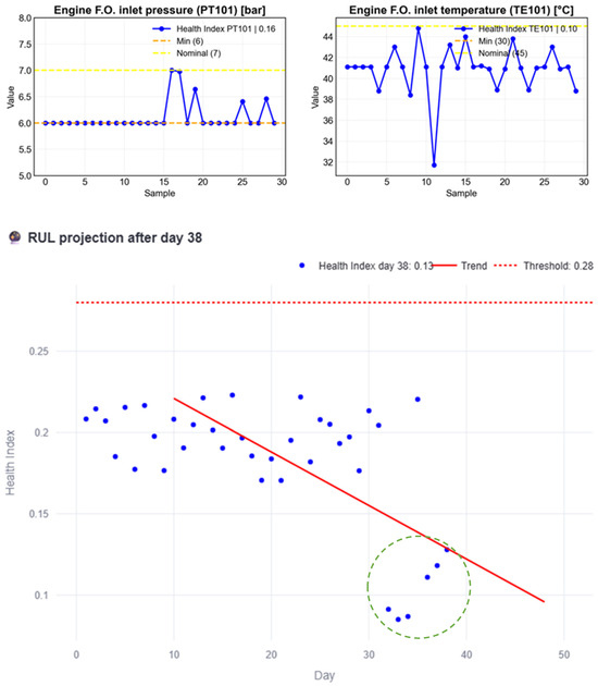
Figure 25. RUL estimation process with the new normal behavior data until day 38.

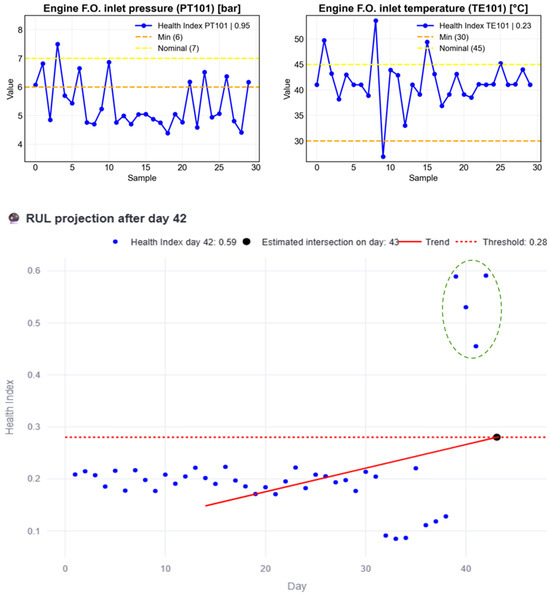
Figure 26. RUL estimation process with the new anomalous behavior data from day 38–42.

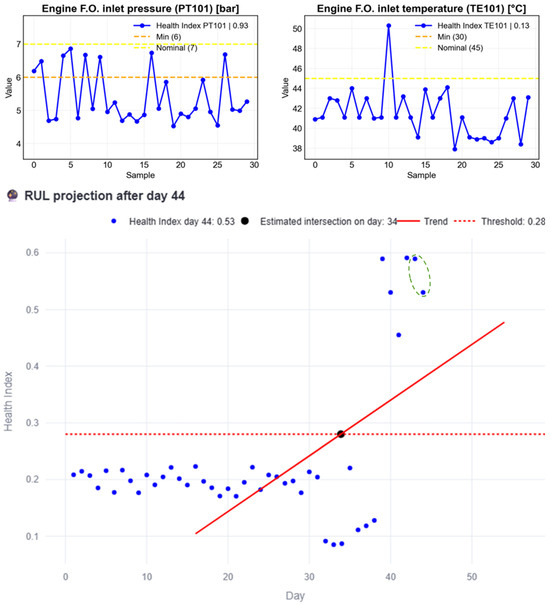
Figure 27. RUL estimation process with the new data when there is no maintenance action after the failure day.

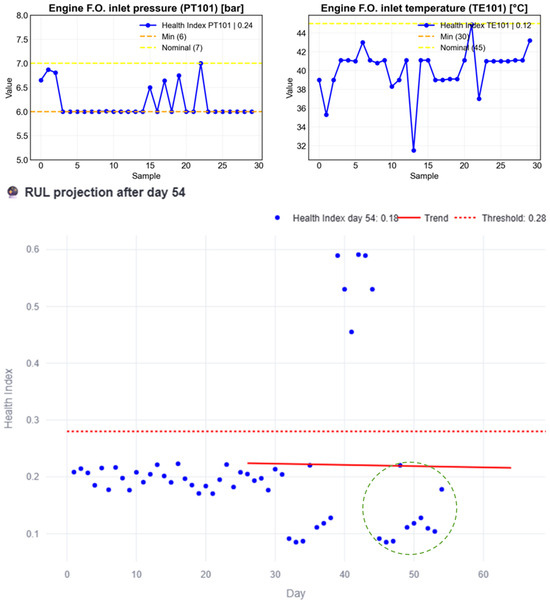
Figure 28. RUL estimation process with the new data after maintenance is done.

Figure 26 shows the effect of introducing anomalous data. As in the original case, an intersection between the trend line and the threshold appears on day 43, based on data up to day 42, resulting in an RUL of 1 day.

Figure 27 illustrates the consequences of not performing preventive maintenance before the estimated failure day, with the anomaly persisting up to day 44, similar to the original dataset.

In contrast, Figure 28 shows that when normal-behavior data is reintroduced—simulating maintenance actions performed by naval personnel after a few days—the intersection disappears, as the normal trend once again dominates.

Figure 29, Figure 30, Figure 31 and Figure 32 present the evolution of RUL over time and the different insights provided to the user at each stage. Figure 29 indicates acceptable subsystem conditions consistent with the normal behavior shown in Figure 25. Figure 30 highlights how the RUL begins to be estimated, since an intersection with the threshold appears in Figure 26, and also shows how the RUL decreases due to the continuous anomalous observations.

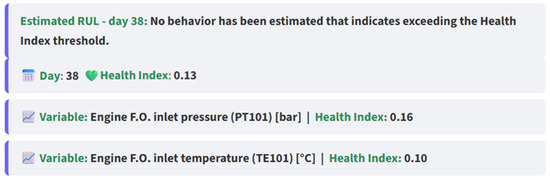
Figure 29. Interface report of the subsystem behavior with the new data up to day 38.

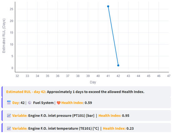
Figure 30. RUL vs. day graph and report based on the RUL estimated with the new data until day 42.

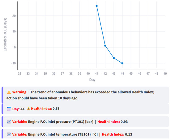
Figure 31. RUL vs. day graph and conclusions based on the RUL with the new data when maintenance is not done.

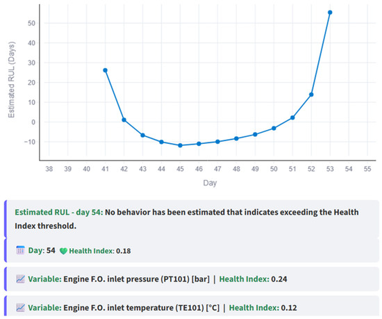
Figure 32. RUL vs. day graph and conclusions based on RUL estimation with the new data after maintenance is done.

Figure 31 reports that maintenance should have been performed earlier, consistent with the results in Figure 27.

Finally, Figure 32 shows how the RUL increases again after the reintroduction of normal-behavior data, following the maintenance actions.

The proposed approach is successfully applied to the new dataset, since it only requires capturing the normal dynamics of the variables, making it a robust data-driven method. The aim of the Experimental Results section is to validate that the methodology can be applied to any set of variables across different groups of components and subsystems. By demonstrating this flexibility, we show that the approach is not limited to a specific set of measurements or to a single type of machinery. Consequently, the methodology could be applied to any machine—whether on the ship or in other industrial settings—as long as the nature of the variables and their operational dynamics are properly understood. This emphasizes the generalizability and practical applicability of our data-driven framework for synthetic data generation and anomaly detection across diverse systems.

5. Conclusions

In this work, a comprehensive software framework for PdM is developed, aimed at estimating the RUL of subsystems in the Wärtsilä 6L26 diesel engine (manufactured by Wärtsilä Italia S.p.A., Trieste, Italy) of the Colombian Navy patrol vessel ARC “20 de Julio” (PZE-46) (manufactured by Colombian Navy, Cartagena, Colombia). The approach is based on the computation of HIs derived from data of variables, enabling a systematic assessment of subsystem degradation over time.

Different state-of-the-art methodologies for synthetic data generation are explored, identifying TVAE as the most suitable technique for this study. These synthetic datasets, emulating normal dynamic behavior of the subsystems, are used to train anomaly detection models. Among several alternatives, we selected a multivariate LSTM Autoencoder approach, which, unlike traditional univariate approaches reported in the literature, allowed us to capture interdependencies between variables within each subsystem.

From the reconstructions obtained, the MAE is computed to derive the HI for each subsystem. By analyzing its temporal trend and performing linear regression, the intersection with the subsystem’s predefined threshold provided an estimate of its RUL. This framework, therefore, offers a practical and scalable methodology for supporting PdM in complex naval engines.

This approach could be successfully applied to the new operational dataset provided by the Colombian Navy because it follows a holistic methodology that operates independently of the specific data source. The only requirement is to capture the normal dynamic behavior of the system variables, which serves as the basis for training. Since the method is fully data-driven, it adapts to different conditions and datasets without relying on predefined models or prior knowledge of the system. The availability of this dataset allowed us to validate the proposed approach with real-world measurements and demonstrate its robustness regardless of the data used for system validation.

For future work, we plan to implement this system on board once the vessel’s sensory and instrumentation infrastructure is fully operational, enabling real-time PdM. Furthermore, we will extend the validation of the proposed framework using publicly available benchmark datasets specifically designed for RUL prediction, which will allow for a broader comparison with other approaches in the field. Additionally, other ways of implementing the proposed approach will be explored, such as testing alternative regression techniques to better capture the trend of the data over time. In parallel, we also plan to investigate different strategies for computing the HI, moving beyond the arithmetic average of the MAE values. For instance, weighted aggregation schemes that account for variable-specific characteristics such as criticality, reliability, or operating range will be tested and compared against the unweighted average. This will enable a more refined and engineering-informed representation of subsystem health, further improving the RUL estimation.

References

- Arena, S.; Florian, E.; Sgarbossa, F.; Sølvsberg, E.; Zennaro, I. A Conceptual Framework for Machine Learning Algorithm Selection for Predictive Maintenance. Eng. Appl. Artif. Intell. 2024, 133, 108340. [Google Scholar] [CrossRef]
- Simion, D.; Postolache, F.; Fleacă, B.; Fleacă, E. AI-Driven Predictive Maintenance in Modern Maritime Transport—Enhancing Operational Efficiency and Reliability. Appl. Sci. 2024, 14, 9439. [Google Scholar] [CrossRef]
- Dueñas-Ramírez, L.M.; Castaño-Restrepo, C.A.; Castiblanco-Tique, S.; Villegas-López, G.A. Success Stories Concerning the Implementation of Predictive Maintenance Through the Use of Industry 4.0 Technologies in Colombian Companies. In Proceedings of the 3rd International Congress on Systems Engineering, Lima, Peru, 2020. [Google Scholar] [CrossRef]
- Tadayon, M.; Pottie, G. TsBNgen: A Python Library to Generate Time Series Data from an Arbitrary Dynamic Bayesian Network Structure. arXiv 2020, arXiv:2009.04595. [Google Scholar] [CrossRef]
- Patki, N.; Wedge, R.; Veeramachaneni, K. The Synthetic Data Vault. In Proceedings of the 3rd IEEE International Conference on Data Science and Advanced Analytics (DSAA), Montreal, QC, Canada, 17–19 October 2016; Institute of Electrical and Electronics Engineers Inc.: New York, NY, USA, 2016; pp. 399–410. [Google Scholar]
- Baressi Šegota, S.; Mrzljak, V.; Anđelić, N.; Poljak, I.; Car, Z. Use of Synthetic Data in Maritime Applications for the Problem of Steam Turbine Exergy Analysis. J. Mar. Sci. Eng. 2023, 11, 1595. [Google Scholar] [CrossRef]
- Mohakul, D.; Kumar, C.R.S.; Singh, S.; Katti, S.; Chougule, S. Health Monitoring of Ship’s Engine with Simulated Data by Using Classifiers -Preliminary Result. In Proceedings of the 2023 2nd International Conference on Electrical, Electronics, Information and Communication Technologies (ICEEICT), Tiruchirappalli, India, 5–7 April 2023; Institute of Electrical and Electronics Engineers Inc.: New York, NY, USA, 2023. [Google Scholar]
- Pinciroli, L.; Baraldi, P.; Zio, E. Maintenance Optimization in Industry 4.0. Reliab. Eng. Syst. Saf. 2023, 234, 109204. [Google Scholar] [CrossRef]
- Ali, A.A.I.M.; Imran, M.M.H.; Jamaludin, S.; Ayob, A.F.M.; Suhrab, M.I.R.; Norzeli, S.M.; Basri, S.B.H.; Mohamed, S.B. A Review of Predictive Maintenance Approaches for Corrosion Detection and Maintenance of Marine Structures. J. Sustain. Sci. Manag. 2024, 19, 182–202. [Google Scholar] [CrossRef]
- Zonta, T.; da Costa, C.A.; da Rosa Righi, R.; de Lima, M.J.; da Trindade, E.S.; Li, G.P. Predictive Maintenance in the Industry 4.0: A Systematic Literature Review. Comput. Ind. Eng. 2020, 150, 106889. [Google Scholar] [CrossRef]
- Kalafatelis, A.S.; Nomikos, N.; Giannopoulos, A.; Trakadas, P. A Survey on Predictive Maintenance in the Maritime Industry Using Machine and Federated Learning. Authorea Preprints 2024. [Google Scholar]
- Susto, G.A.; Schirru, A.; Pampuri, S.; McLoone, S.; Beghi, A. Machine Learning for Predictive Maintenance: A Multiple Classifier Approach. IEEE Trans. Industr. Inform. 2015, 11, 812–820. [Google Scholar] [CrossRef]
- Kalafatelis, A. A Lightweight Predictive Maintenance Strategy for Marine HFO Purification Systems. In Proceedings of the 21 st European, Mediterranean, and Middle Eastern Conference on Information Systems, Athens, Greece, 2–3 September 2024. [Google Scholar] [CrossRef]
- Orhan, M.; Celik, M. A Literature Review and Future Research Agenda on Fault Detection and Diagnosis Studies in Marine Machinery Systems. Proc. Inst. Mech. Eng. Part M J. Eng. Marit. Environ. 2024, 238, 3–21. [Google Scholar] [CrossRef]
- Velasco-Gallego, C.; Lazakis, I. RADIS: A Real-Time Anomaly Detection Intelligent System for Fault Diagnosis of Marine Machinery. Expert Syst. Appl. 2022, 204, 117634. [Google Scholar] [CrossRef]
- Githinji, S.; Maina, C.W. Anomaly Detection on Time Series Sensor Data Using Deep LSTM-Autoencoder. In Proceedings of the IEEE Africon Conference, Nairobi, Kenya, 20–22 September 2023; Institute of Electrical and Electronics Engineers Inc.: New York, NY, USA, 2023. [Google Scholar]
- Faggioni Nicolo, N.; Caviglia, A.; Guarnera, N.; Schininà, E.; Sansebastiano, E.; Chiti, R. Enhancing Predictive Maintenance in the Maritime Industry with Unsupervised Learning. In Proceedings of the International Ship Control Systems Symposium, Liverpool, UK, 5–7 November 2024; Institute of Marine Engineering Science & Technology: London, UK, 2024. [Google Scholar]
- Lachekhab, F.; Benzaoui, M.; Tadjer, S.A.; Bensmaine, A.; Hamma, H. LSTM-Autoencoder Deep Learning Model for Anomaly Detection in Electric Motor. Energies 2024, 17, 2340. [Google Scholar] [CrossRef]
- DataCebo, Inc. Synthetic Data Metrics; DataCebo, Inc.: Boston, MA, USA, 2023. [Google Scholar]
- Palacio-Niño, J.-O.; Berzal, F. Evaluation Metrics for Unsupervised Learning Algorithms. arXiv 2019, arXiv:1905.05667. [Google Scholar] [CrossRef]
- West, R.M. Best Practice in Statistics: Use the Welch t-Test When Testing the Difference between Two Groups. Ann. Clin. Biochem. 2021, 58, 267–269. [Google Scholar] [CrossRef] [PubMed]
Disclaimer/Publisher’s Note: The statements, opinions and data contained in all publications are solely those of the individual author(s) and contributor(s) and not of MDPI and/or the editor(s). MDPI and/or the editor(s) disclaim responsibility for any injury to people or property resulting from any ideas, methods, instructions or products referred to in the content. |
© 2025 by the authors. Licensee MDPI, Basel, Switzerland. This article is an open access article distributed under the terms and conditions of the Creative Commons Attribution (CC BY) license (https://creativecommons.org/licenses/by/4.0/).