Abstract
Agent based modelling has been widely accepted as a promising tool for urban planning purposes thanks to its capability to provide sophisticated insights into the social behaviours and the interdependencies that characterise urban systems. In this paper, we report on an agent based model, called TransMob, which explicitly simulates the mutual dynamics between demographic evolution, transport demands, housing needs and the eventual change in the average satisfaction of the residents of an urban area. The ability to reproduce such dynamics is a unique feature that has not been found in many of the like agent based models in the literature. TransMob, is constituted by six major modules: synthetic population, perceived liveability, travel diary assignment, traffic micro-simulator, residential location choice, and travel mode choice. TransMob is used to simulate the dynamics of a metropolitan area in South East of Sydney, Australia, in 2006 and 2011, with demographic evolution. The results are favourably compared against survey data for the area in 2011, therefore validating the capability of TransMob to reproduce the observed complexity of an urban area. We also report on the application of TransMob to simulate various hypothetical scenarios of urban planning policies. We conclude with discussions on current limitations of TransMob, which serve as suggestions for future developments.
1. Introduction
The growing population in many parts of the world is highly urbanised and the complexity of large cities make urban planning increasingly challenging. Urban planners need not only tools that help realistically predict the demands of the urban population (e.g., transport and housing), but more importantly those that give sophisticated insights into social behaviours and the interdependencies that characterise urban systems. Traditional and widely applied Land Use Transport (LUT) models are relatively computationally inexpensive and comprehensive in simulating the spatial dependency between land use and transport planning. They are however nondynamic, failing to capture the processes (i.e., learning and decision making) that are instrumental to social behaviours and thus unable to provide a microscopic view of urban systems [1]. Agent based modelling, with its ability to computationally reproduce individuals and households together with their characteristics and behaviours, has been widely adapted in assisting urban planning process.
Indeed agent based models for urban planning purposes have been increasingly introduced over the last decades. Miller et al. [2] developed the ILUTE (Integrated Land Use, Transportation, Environment) software to simulate the evolution of the whole Toronto region in Canada with approximately 2 million households and 5 million people over an extended period of time. Besides giving useful information to analyse a wide range of transport and other urban policies, ILUTE also explicitly models travel demand as an outcome of the integration between individual and household decisions based on activities that they commence during a day. Raney et al. [3] presented a multi-agent traffic simulation for all of Switzerland with a population of around 7 million people. Balmer et al. [4] demonstrated the flexibility of agent based modelling by successfully developing an agent based model that satisfactorily simulate the traffic demands of two scenarios: (i) Zurich city in Switzerland with 170 municipalities and 12 districts; and (ii) Berlin/Brandenburg area in Germany with 1008 traffic analysis zones. Many other agent based models for transport and urban planning can be found in the literature, with different geographical scales and at various levels of complexity of agent behaviours and autonomy [5,6,7,8,9,10,11,12,13,14]. They proved that with a large real world scenario, agent based modelling, while being able to reproduce the complexity of an urban area and predict emergent behaviours in the area, can have no significant performance issues [12]. They also show that for traffic and transport simulation purposes, agent based modelling has been considered as a reliable and well worth developing tool that planners can employ to build and evaluate alternative scenarios of an urban area. It is worth noting that in many models that have been reported in the literature, the dynamic interactions between demographic evolution, the resulting transport/traffic demands, and residential mobility (and thus housing demands) were not explicitly simulated. In a bid to bridge that gap, we propose in this paper an agent based model that encapsulates such dynamics and, more importantly, the resulting changes in the liveability perception of the population in an urban area. The model, called TransMob, was developed to capture the population and its dynamics for a metropolitan area in South East Sydney in New South Wales (NSW), Australia. The underlying modelling framework however is transferable and readily applicable for modelling any (larger) area and population provided that the supporting data is available.
Individuals are represented in this model as autonomous decision makers that make decisions affecting their environment (i.e., travel mode choice and relocation choice) as well as decisions in reaction to changes in their environment (e.g., family situation, employment). More importantly, they are associated with each other by their household relationship, which not only define interdependencies of their transport demands and housing needs but constrain their decision makings (e.g., in relation to transport mode and residential relocation). With respect to transportation, each individual has a travel diary, which comprises a sequence of trips the person makes in a representative day as well as trip attributes including origin, destination, travel mode, trip purpose, and departure time. The actual travel time of trips on the road network (e.g., by private cars) in the study area is simulated by a novel traffic micro-simulator, where each agent has a neural network that perceives local traffic condition and then this allows for the dynamic re-routing of trips during the simulation. Outputs of the traffic micro-simulator (e.g., actual travel time and traffic density) then partly inform the decision making of an individual of transport mode choice and change in his/her liveability perception of the neighbourhood.
The remaining of the paper is organised as below. The six major computational modules that constitute TransMob, including the novel traffic micro-simulator, are presented in Section 2. Please note that details of these six modules have been peer-reviewed and published elsewhere, and thus enhance the credibility of TransMob. Section 2 therefore gives only an overview of their functionality and how they were developed. The prime purpose of the present paper is reporting how these individual modules fit together for integrated simulation and analysis of the dynamics of an urban system. Section 3 presents the validation of TransMob against a number of survey datasets including demographics attributes, transport demands, and housing demands. Section 4 demonstrates the application of TransMob for exploratory study of emergent behaviours of an urban area via a number of hypothetical scenarios of planning policies. Section 5 discusses limitations in the current version of TransMob and suggestions for future developments.
2. Computational Modules of TransMob
Six major modules interacting with each other constitute the core of TransMob: Synthetic population, Perceived liveability, Travel diaries, Traffic micro-simulator, Transport mode choice and Residential relocation choice. These six modules are designed to capture the mutual dynamics of key elements of an urban area with regards to transport and land use. More specifically, thanks to these modules, TransMob is able to predict the change of demographics in the urban area of interest, how this change impacts housing and transport needs of the population and the way they make collective decisions regarding relocation. The traffic micro-simulator enables TransMob to translate such transport needs of the population into traffic density on the road network and the travel experience of the population (in terms of travel time). TransMob uses this information not only to update the individuals’ satisfaction to their neighbourhood, but also to help individuals and households make their travel mode decisions.
An overview of each of the modules, the interactions between them along with their supporting dataset are given in Figure 1 and the subsections below. The datasets required are the Census data, the Journey to Work (JTW) data, the Household Travel Survey (HTS) data, Computer Assisted Telephone Interviewing (CATI) data, Geospatial Information System (GIS) data of the road network and the Household, Income and Labour Dynamics in Australia (HILDA) data. Extensive details on the TransMob architecture and integration of these modules are given in [15].
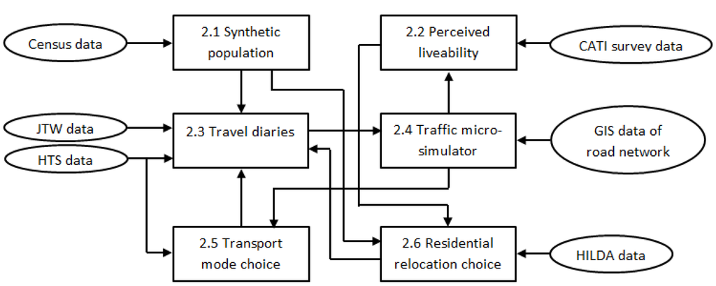
Figure 1.
Computational modules of TransMob.
Figure 1.
Computational modules of TransMob.

2.1. Synthetic Population
A synthetic population is instrumental in any agent based model that simulates social behaviours particularly in relation to transport and residential mobility. The synthetic population in TransMob serves the same purpose as its counterpart did in agent-based models for transport and land use simulation previously reported in the literature [2,3,4,5,6,7,8,9,10,11,12,13,14]. More specifically, it is a valid computational representation of the real population in the study area that matches the distribution of individuals and households as per the demographics from census data. The synthetic population module in TransMob is responsible for two tasks, constructing the initial synthetic population and evolving the synthetic population at every simulation step.
The algorithm constructing initial population in TransMob follows the sample-free approach and is among the very few in the literature that do not rely on a sample survey data to construct a synthetic population, even though it can take advantage of such data to improve the quality of the synthetic population. The generator relies solely on aggregated demographics attributes of the target area (i.e., tables in census data) and is further constrained by biological laws (e.g., the mother-child age gap). The resulting population comes in the form of disaggregated records, each represents a synthetic individual characterised by six attributes including age, gender, household relationship, household type, identification of the synthetic household he/she belongs to, and the identification of the travel zone the synthetic household resides in. Full details on the algorithm for constructing a synthetic population for agent based modelling purposes that was used in TransMob can be found in [16]. Travel zones are geographical units that the Bureau of Transport Statistics (Transport for NSW, Australia) used at the time the model was developed for data collection, transport modelling and analysis. Key land use attributes defining travel zones include employment, housing and transport infrastructure. For trip generation purposes, travel zones are configured so that they are relatively smaller for areas with high land use densities and larger for those with lower densities [17]. In TransMob, travel zones are used as geographical unit for the modelling and analysis of transport demand (e.g., informing the location of trip destinations), perceived liveability and residential relocation choices of individuals and households.
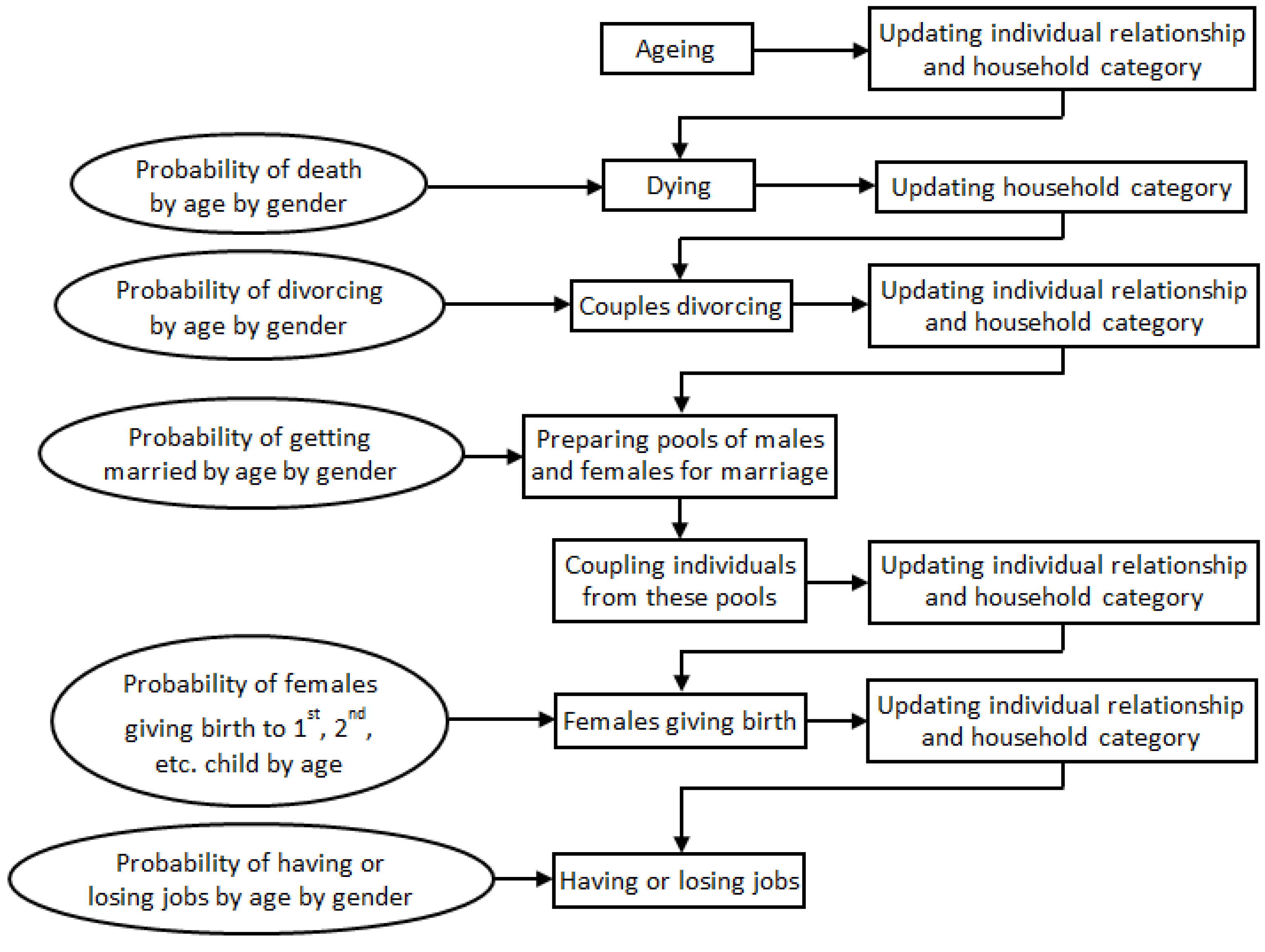
The evolution of the synthetic population involves the aging of each individual and the simulation of age-dependent life events (death, birth, divorce, and marriage). The occurrence of these life events influences both individuals as well as household entities, i.e., the consequent changes in the structured of households as a results of individual evolution are captured. A divorced couple, for example, creates a new household one of the divorcees will move into. The existing household and remaining residents will have their relationship status changed accordingly, so do their transport and housing needs. The evolution steps are summarised in Figure 2. Full details of the evolution algorithms can be found at [18]. An immigration population may be added to the existent population of the study area at the end of each simulation step.
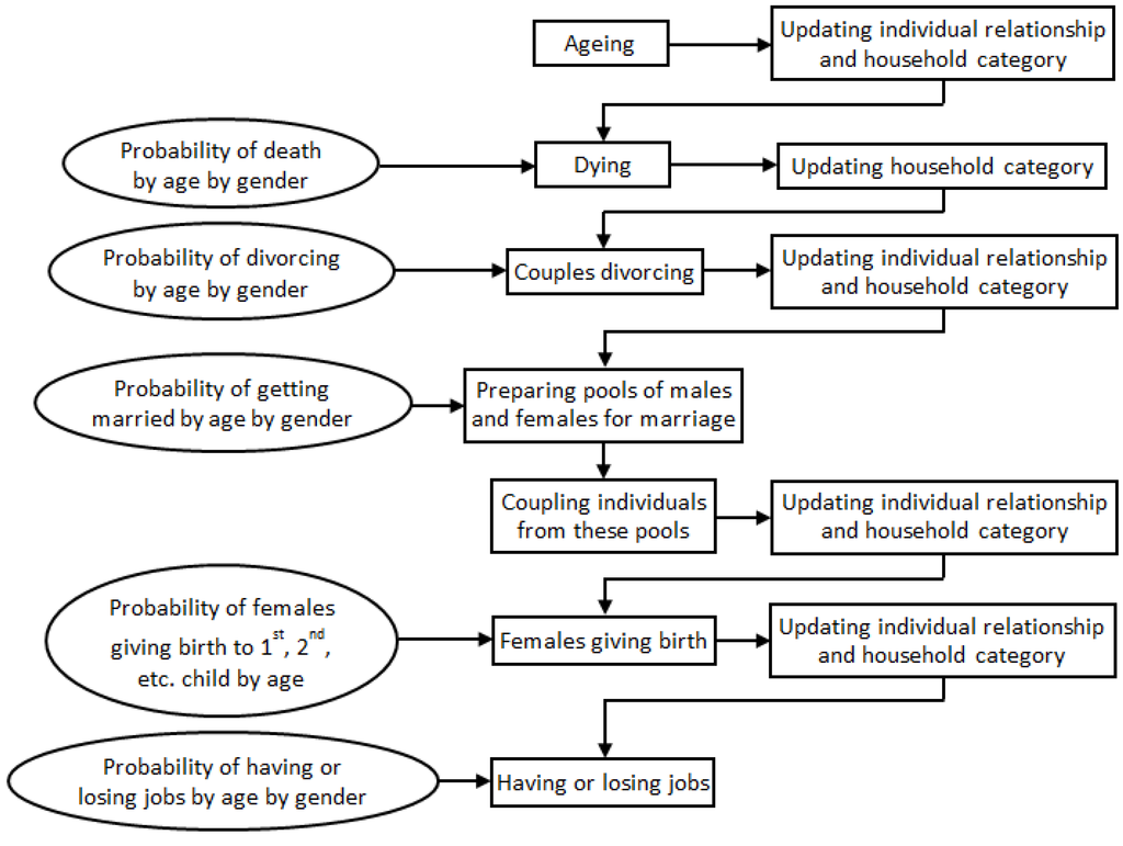
Figure 2.
Steps of synthetic population evolution.
Figure 2.
Steps of synthetic population evolution.
2.2. Perceived Liveability
A significant departure of the current model to other existing approaches is the assumption that residential location choice is based not only on availability and affordability principles but also on the perception that individuals have of the quality of the environment in which they live. The perceived liveability component uses a semi-empirical model to estimate individual levels of attraction to and satisfaction with specific locations. The semi-empirical model is a statistical weighted linear model calibrated on a CATI survey data collected in the study area. Full details of the survey and the semi-empirical model built from the model can be found in [19,20].
2.3. Travel Diaries
Each individual in the synthetic population is assigned with a travel diary which comprises a sequence of trips the person makes in a representative day as well as trip attributes such as travel mode, trip purpose, departure time, origin and destination. Because these details of travel behaviours of the population are not completely available in any single source of data (for confidentiality reasons), the process of assigning travel diaries to individuals comprises two steps. The first step assigns a trip sequence each individual makes in a representative day using the HTS data. Details of each trip in this trip sequence include trip purpose, travel mode, and departure time. The second step assigns locations to the origin and destination of each trip in the trip sequence, supported by the JTW data. Full details of semi-deterministic algorithm that assigns trip sequence to a synthetic individual are given in [21]. Full details of an algorithm that allocates origin and destination to trips, as well as an algorithm for updating travel diaries of the evolved population at every simulation step are given in [22].
2.4. Traffic Micro-Simulator
Traffic flows simulation is the natural follow up of the travel demand forecast (i.e., travel diaries) performed in Section 2.3. The traffic micro-simulator is in charge of executing the daily plans of the agents, hence reproduce the dynamics of traffic density on the road network. It resembles the central part of established traffic micro-simulators such as MATSim [23], TRANSIMS [24], DynaMIT [25] and AIMSUN [26].
The aforementioned traffic micro-simulators typically compute a (stochastic) user equilibrium by means of iterative simulations. These successive steps generate traffic flows until the travel time of each agent becomes stationary. At the end of every step, the performance of each agent is assessed and the micro-simulator modifies the plans of the most problematic agents (e.g., by assigning a new path or modifying the departure time). Consequently this iterative nature might results in a high computational cost, in particular when the number of agents is large and/or the road network is complex [27]. Furthermore these equilibrium approaches rely on strong assumptions and have several limitations now well identified [28]. Hence we opt for a behavioural approach in building a traffic micro-simulator in this study.
An original dynamic traffic assignment (DTA) model relying on reactive and autonomous agents has then been chosen as the traffic-micro simulator in TransMob. This new DTA scheme relies on the assumption that travellers take routing policies rather than paths: each agent has the ability to apply a strategy letting him or her to possibly re-route his/her path depending on the perceived local traffic conditions and time already spent travelling. The re-routing process allows the agents to be truly autonomous as they can directly react to any change in the road network, a major deviation from the more classical approaches where the agents follow predefined plans. This ability given to the agents removes the need of restarting the whole simulation process and consequently decreases the computational cost with respect to more classical equilibrium approaches. For the sake of simplicity, the strategy is modelled using a simple neural network [29]. The inputs of such neural network read the local information about the road network and the output gives the action to undertake, stay on the same path or modify it. As the agents use only local information, the overall road network topology does not really matter, thus the strategy is able to cope with large road networks, i.e., the model is highly scalable [29].
The micro-simulator current implementation relies on the C++ programming-language-based Repast for High Performance Computing (HPC) modelling platform [30]. The outcome is a highly efficient software being able to run on simple workstation as well as HPC facilities, taking advantage of their multiple computational cores. For instance, the simulation of 100,000 agents performing a total number of 360,000 trips over a day (24 h period) and moving across a road network consisting of 7000 nodes and 17,000 links required only 1/16th of the computational time needed by TRANSIMS for a single iteration (The numerical experiments for TRANSIMS and our model have been performed on an Intel® Core™ i5-4570 with 16 GB of RAM). More specifically on the computational time, TRANSIMS took approximately 24 h for one iteration, MATSim took around 0.5 h for 20 iterations and our behavioural traffic micro-simulator took 1.5 h for one iteration.
2.5. Transport Mode Choice
The purpose of the travel mode choice algorithm is to accurately describe the decision-making processes of individuals travelling on the transport network in the study area, thus enabling the prediction of the choice of travel modes of individuals in the population. Travel modes considered in this study are car driver, car passenger, public transport, taxi, bicycle, walk, and others.
A multinomial logit (MNL) model is developed for this purpose. At the heart of the MNL formulation is a linear part-worth utility function that calculates the utility of each alternative travel mode choice. Independent variables for this function include the difference of fixed cost and difference of variable cost of the selected travel mode with the cheapest mode [31]. The variable cost is dependent on the estimated travel time, which is the output of the traffic micro-simulation. Another independent variable is the individual’s income, acting as a proxy for the individual’s perception of value of time. Multinomial logit regression is used on the HTS data to estimate the utility coefficients vector for the possible travel modes. Full details on the development of this multinomial logit model for transport mode choice can be found in [32].
2.6. Residential Relocation Choice
Household relocation modelling is an integral part of both the residential and transport planning processes, as household locations determine demand for community facilities and services, including transport network demands. The approach used to model residential location choice includes two distinct processes: the decision to relocate, and the process of finding a new dwelling. A multinomial logit model is used to represent the process by which households make decision to relocate. The attributes of this model are change in household income, change of household configuration (e.g., having a newborn, divorced couples, newly wed couples), and the tenure of the household. The data from the HILDA survey is used to regress the coefficients associated to each of these attributes needed in the binomial logit model. Full details on the development of the model for triggering household relocation can be found in [33].
Once a household is selected for relocation, the second decision determines where the household will relocate and whether they will be renting or buying a dwelling in the target location, if a suitable dwelling is found. This process of finding a new dwelling is modelled as a constraint satisfaction process, whereby each household will attempt to find a suitable dwelling based on three factors, availability, liveability, and affordability.
With regards to housing availability, the initial simulated dwelling stock for four categories of house size (1 bedroom, 2 bedrooms, 3 bedrooms, and more than 3 bedrooms) is calibrated from the census data in 2006 and distributed across all travel zones. The dwelling stock from census data in 2011 is used to interpolate the dwelling availability in each year in between and into the future (via linear extrapolation). Alternatively, TransMob accepts user input for dwelling stocks in each dwelling category (house size) for each travel zone to facilitate the examination of housing supply scenarios. These user-input tables of housing stock will override the interpolated/extrapolated data.
With regards to dwelling pricing model, the sale and rental prices in travel zones in the study area are determined from the data provided by the Bureau of Transport Statistics (part of the Government department known as Transport for New South Wales, Australia) on the average sale prices. The Rent and Sales Report published by the New South Wales Department of Family and Community Services is also used to approximate the sale and rental price for different house size categories. In the current version of TransMob, the house prices are kept static over time, a limitation of our model due to the lack of data.
The algorithm for simulating the process of finding a dwelling of a household is presented in Figure 3. First the house size (in terms of number of bedrooms) required by the relocating household is heuristically decided based on the number of adults (over 15 years old), whether they are a couple, and the number of children in the household. It is assumed in TransMob that the relocating household will look for houses that have the number of bedrooms equal to or maximum of one higher than the number bedrooms required. Travel zones with at least one vacant dwelling satisfying this dwelling size is added into a list of travel zones to be considered. The relocating household then looks into the most liveable travel zone in the list and decides if it can afford to buy a property there. If not, it searches into the next most liveable travel zone, and so on. If the household cannot afford buying any property in the listed travel zones, it will then re-search the list, starting with the most liveable ones, for a property that it can afford to rent. If eventually the relocating household is unable to afford to either buy or rent a property in any of the listed travel zones, it is considered relocated to outside of the study area and is removed from the model.

Figure 3.
Algorithm for simulating the search for an affordable dwelling of a relocating household.
Figure 3.
Algorithm for simulating the search for an affordable dwelling of a relocating household.
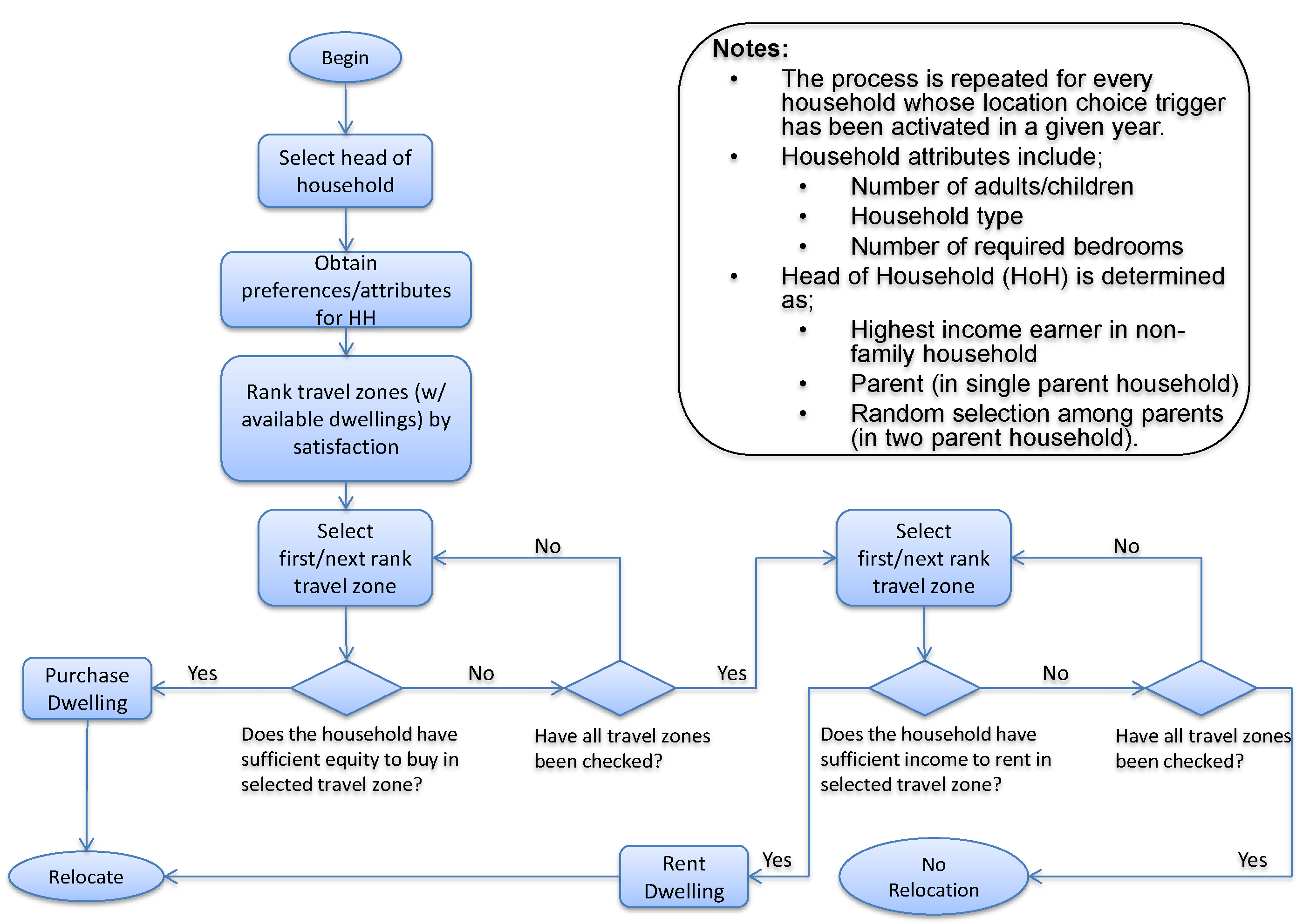
Note that the modelling of dwelling affordability of a household is simplified in TransMob to ensure the correct focus is placed in the target dynamics of residential relocation choice. The purpose of the model is not to measure the economic dynamics of housing markets, but rather the residential migration rates and mobility patterns. To this end, a simple algorithm has been used to account for cumulative equity of a household. If a household is paying mortgage, the mortgage repaid is added to its equity at the end of each simulation step. If a household is renting, it has savings that will be used in considerations of buying a property in the future simulation steps. This savings rate is assumed one third of household income per annum, in line with [34]. In the search for an affordable property to relocate (as described in Figure 3), a household compares its weekly total income with the weekly mortgage payment or rental cost. If the household’s weekly income is higher than the repayments on the dwelling price (including stamp duty) with an assumed 7% interest, distributed using the standard monthly payment formula on a fixed rate mortgage over a nominal thirty-year payment period, then the dwelling is deemed affordable for purchase. If the income is not greater than the estimated mortgage payment, but is greater than the rental cost, the dwelling may be rented. Over time, changes in household income will only occur when individuals in the household change employment status as decided as part of the synthetic population evolution (described in Section 2.1). Given that household costs remain static over time in our model (due to a lack of data), this formulation will not lead to any significant rises or decreases in the number of affordable dwellings available to a household as income will not change unless an individual in the household changes job. This model of dwelling affordability is acknowledged to be a gross simplification of the process of residential relocation. However, given that the focus of the model is to provide representative impacts of residential relocation, it is considered that these assumptions are valid for the purposes of the model.
3. Validations of Simulation Results
TransMob is applied to simulate the dynamic interactions between population growth, transport demands and urban residential mobility for a metropolitan area consisting of Randwick and Green Square in the south east of Sydney, Australia. The simulation period is from 2006 to 2011, the year that we last have census data for, where each simulation step represents a year. For each year, however, the simulation is carried out for one representative day. It is for this day that the travel patterns of the population are modelled and simulated. Variation of the travel patterns from one day to another (due to weather or mood swing for example) is not informed in the Household Travel Survey Data (which is the main data source for modelling travel demand in this study), or anywhere else, and thus is not simulated in TransMob. We acknowledge that there are likely considerable differences between travel patterns of a representative weekday and those of a representative weekend. Modelling travel patterns of a representative weekend will be considered as part of future developments of TransMob.
Having said that, the insights that are gained from studying/modelling the travel patterns of a representative workday would be sufficient for urban transport planning purposes. This is because workdays normally have the majority in a calendar year, normally have higher travel demands and thus pose more stress on the road network compared to weekend and holidays. Also such limitation is fine for a simulation model for strategic planning purposes. The impacts of travel patterns due to special events (e.g., carnivals) can be studied by designing a specific scenario inputted into TransMob.
In order to validate the capability of TransMob in reproducing observed complexity of an urban area, the final simulation results are rigorously compared against all the real life datasets available in 2011 across various attributes of the study area, including population demographics, housing structures, transport demands, and road traffic density.
3.1. Validation of Population Demographics
The study area has approximately 106,000 individuals living in around 48,000 households that reside in private dwellings. The initial population is constructed using the 2006 census data, released by the Australian Bureau of Statistics (ABS). This initial synthetic population is validated by Huynh et al. [18] that it matches the demographics of the real population at both individual level and household level, and thus is a realistic computational representation of the real population in the study area [18].
The demographics of the synthetic population at the end of the simulation are compared against the census data of the study area available in 2011 (released by ABS) at both individual level (Figure 4) and household level (Figure 5). Please note that census data in 2011 is the latest that can be used to validate the demographics evolution from 2006. The next census will not be available until 2016, which we are keen to use to further validate the evolution. A full description of household types being simulated in TransMob using the household types as given in the source census data is listed in Table 1.
Note that due to the lack of relevant data and in order to preserve the demographics at the household level, we assume a net 300 households equally distributed across the 17 household types immigrating into the study a year. These households are randomly drawn from the initial synthetic population (year 2006) and added to the population in each year. TransMob also accepts user input for the demographics of immigrants in each year to allow for the examination of changes of demographic structure due to immigration policies. Such user input will overwrite the default values of immigrants predefined in the model.
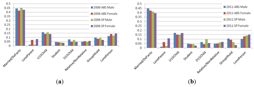
Figure 4.
Proportion of males and females by household relationship in study area in (a) 2006 and (b) 2011.
Figure 4.
Proportion of males and females by household relationship in study area in (a) 2006 and (b) 2011.
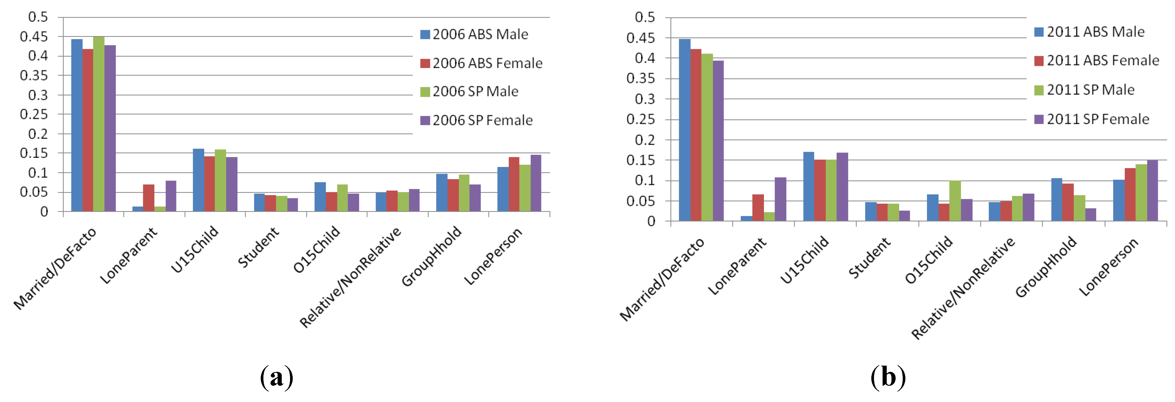
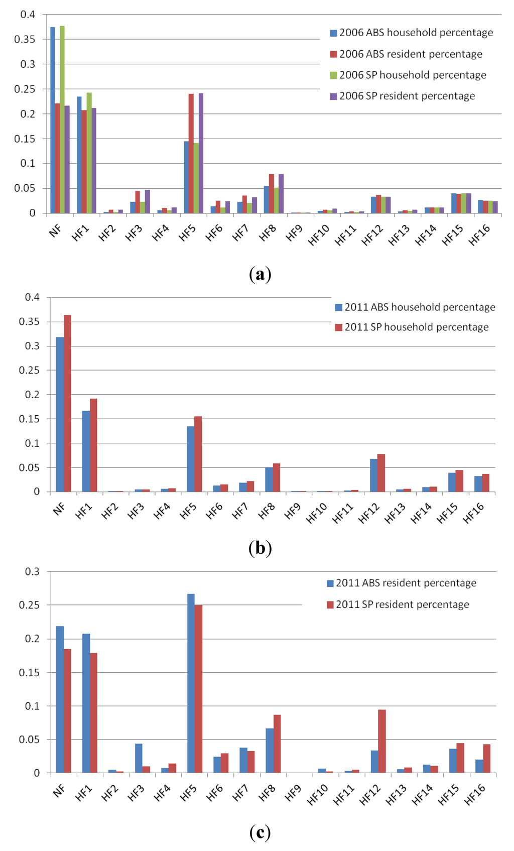
Figure 5.
Proportion of household types in study area (a) in 2006 by number of residents and number of households; (b) in 2011 by number of households; (c) in 2011 by number of residents.
Figure 5.
Proportion of household types in study area (a) in 2006 by number of residents and number of households; (b) in 2011 by number of households; (c) in 2011 by number of residents.


Table 1.
Household type in census data and their denotation in the synthetic population in TransMob.
| Census Data | Denotation in Synthetic Population |
|---|---|
| Couple family with no children | HF1 |
| Couple family with children under 15 and | |
| dependent students and non-dependent children | HF2 |
| dependent students and no non-dependent children | HF3 |
| no dependent students and non-dependent children | HF4 |
| no dependent students and no non-dependent children | HF5 |
| Couple family with no children under 15 and | |
| dependent students and non-dependent children | HF6 |
| dependent students and no non-dependent children | HF7 |
| no dependent students and non-dependent children | HF8 |
| One parent family with children under 15 and | |
| dependent students and non-dependent children | HF9 |
| dependent students and no non-dependent children | HF10 |
| no dependent students and non-dependent children | HF11 |
| no dependent students and no non-dependent children | HF12 |
| One parent family with no children under 15 and | |
| dependent students and non-dependent children | HF13 |
| dependent students and no non-dependent children | HF14 |
| no dependent students and non-dependent children | HF15 |
| Other family | HF16 |
| Non family household | NF |
The comparisons in Figure 4 and Figure 5 show that TransMob, while simulating the evolution of the population discretely at individual level, is able to predict reasonably well the demographic distributions of the whole population in 2011. More specifically, Figure 4 shows that in 2011, synthetic households of types NF, HF1, and HF5 maintain relatively higher proportions in the population compared to other household types. The figure also shows a slight drop in the proportions of household types HF3 and HF12 compared to 2006, whereas those of other household types remain relatively unchanged. At an individual level, TransMob successfully predicts that individuals in a relationship (married or de facto) occupy a higher proportion in the population compared to other individual types. The proportions of lone parents are relatively much lower, with significantly higher number of female lone parents compared to male lone parents.
However, there are mismatches in the simulation results of evolution compared to the 2011 census data. For example, TransMob fails to match the proportions of group household members and lone persons. It is also unable to predict the drop of non-family households in 2011 compared to 2006. These deviations could be attributed to a number of factors. Firstly, the age dependent evolution rates that drive the evolution through each of the 5 years in the simulation are for the whole of Australia in 2006. These rates thus when applied to the population in a much smaller urban area are prone to produce discrepancies between the predicted population and the census data for the area. The evolution algorithm in its current design is also unable to capture the complexity in the dynamics of urban households, for example adult children leaving their parent’s house, and the formation of three (or) more generation households.
3.2. Validation of Housing Structures
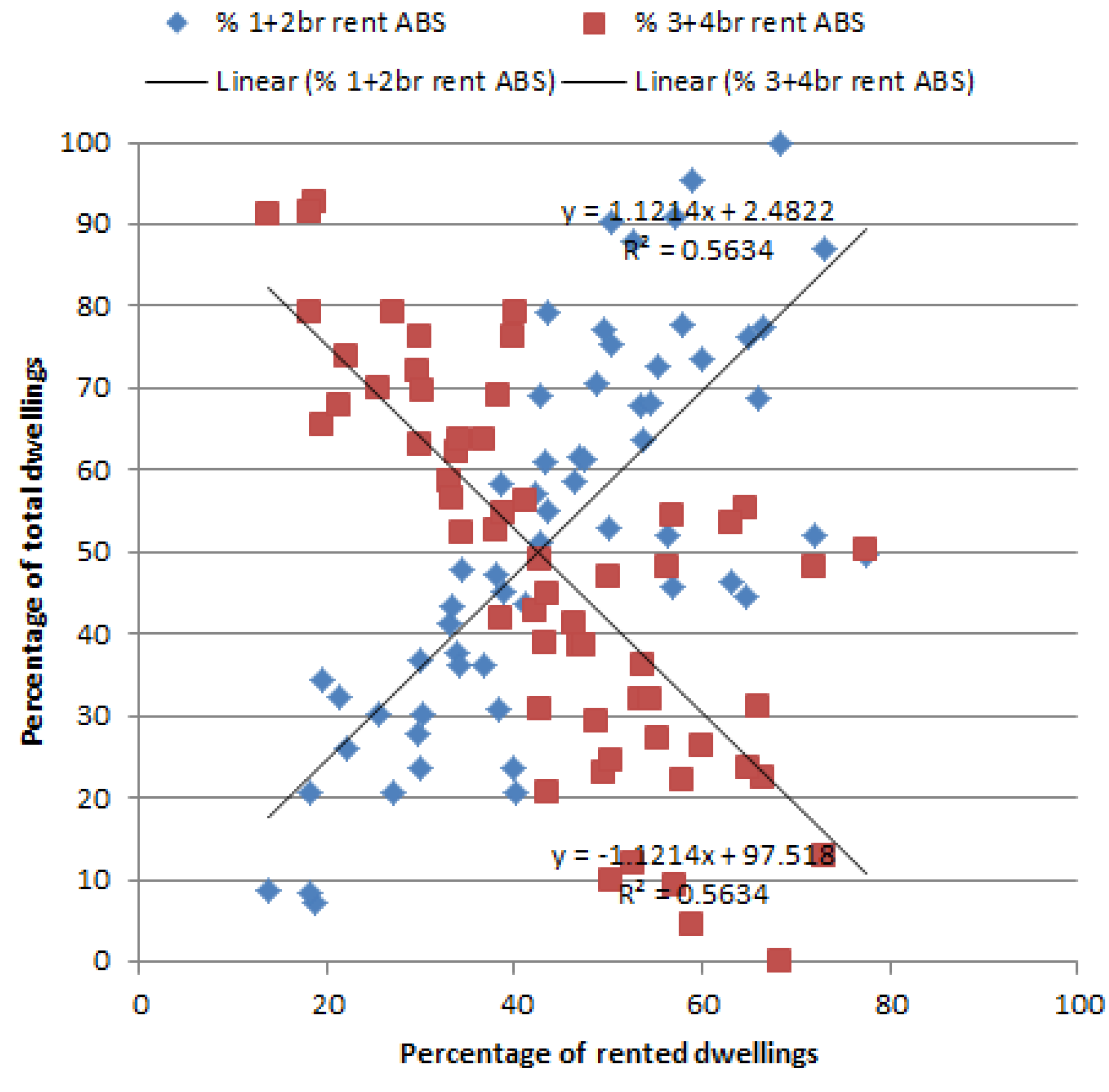
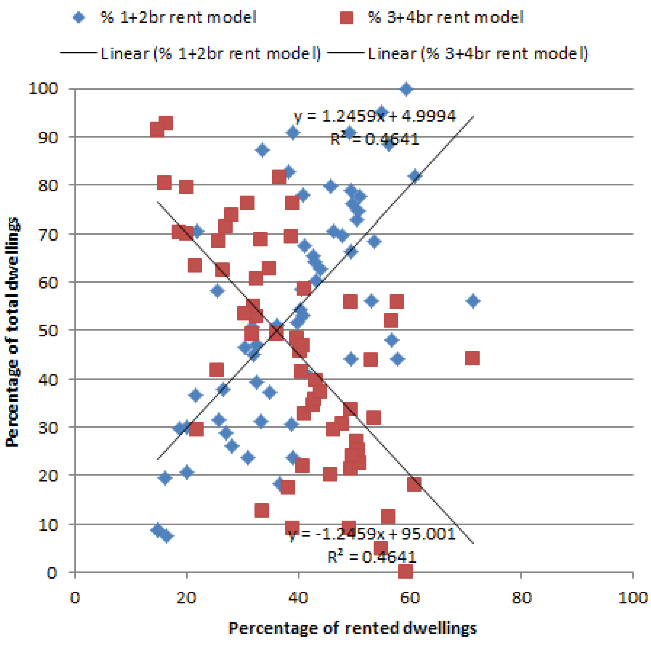
Based on the 2011 census data on ownership status by number of bedrooms by travel zones (released by ABS), the relation between the percentage of small dwellings in a travel zone and the percentage of small dwellings being rented in that travel zone is plotted for all travel zones in the study area (blue dots in Figure 6). The same relation for large dwellings is also plotted in Figure 6 (red dots). We define small dwellings as those having two or less bedrooms, and large dwellings as those having three bedrooms or more. The two sets of data points show that across the study area, travel zones that have a smaller proportion of small houses tend to have less of them occupied under a rental arrangement. The opposite trend applies to larger dwellings, i.e., travel zones that have a larger proportion of larger dwellings tend to have more of them occupied by homeowners.

Figure 6.
Distribution of rented dwellings by house size for travel zones in study area in census (ABS) data for 2011.
Figure 6.
Distribution of rented dwellings by house size for travel zones in study area in census (ABS) data for 2011.
The two distributions for small and large dwellings from the simulation results are plotted in Figure 7, which reflect the same trends that are observed in census data. This validates that the (simplified) algorithm of housing affordability in TransMob can reasonably reproduce the reasoning processes of people when choosing relocating to a new house. It is, however, not perfect, particularly with the assumptions that we made (see Section 2.6), and this explains the deviations between the simulation results and the census data. These assumptions, particularly on house prices and household equity, can be relaxed provided relevant data is made available to the model.

Figure 7.
Distribution of rented dwellings by house size for travel zones in study area from TransMob for 2011.
Figure 7.
Distribution of rented dwellings by house size for travel zones in study area from TransMob for 2011.
3.3. Validation of Travel Demands
Figure 8 and Figure 9 respectively show the percentage of trips by travel mode and trip purpose with respect to the number of trips made by the whole population for year 2006 (initial year) and year 2011 (the final simulation year). Figure 10 compares the percentage of individuals in the synthetic population against that in the HTS data by the number of trips made daily. The distributions of simulation results in these graphs are in very good agreement with the HTS data for the whole Sydney Greater Metropolitan Area. Note that the HTS data used for comparisons in Figure 8 to Figure 10 is the collective data of years from 2006 to 2011. This is to comply with the suggestion that three or more years of data are pooled to give reliable estimates of travel at a particular geographical level [35].
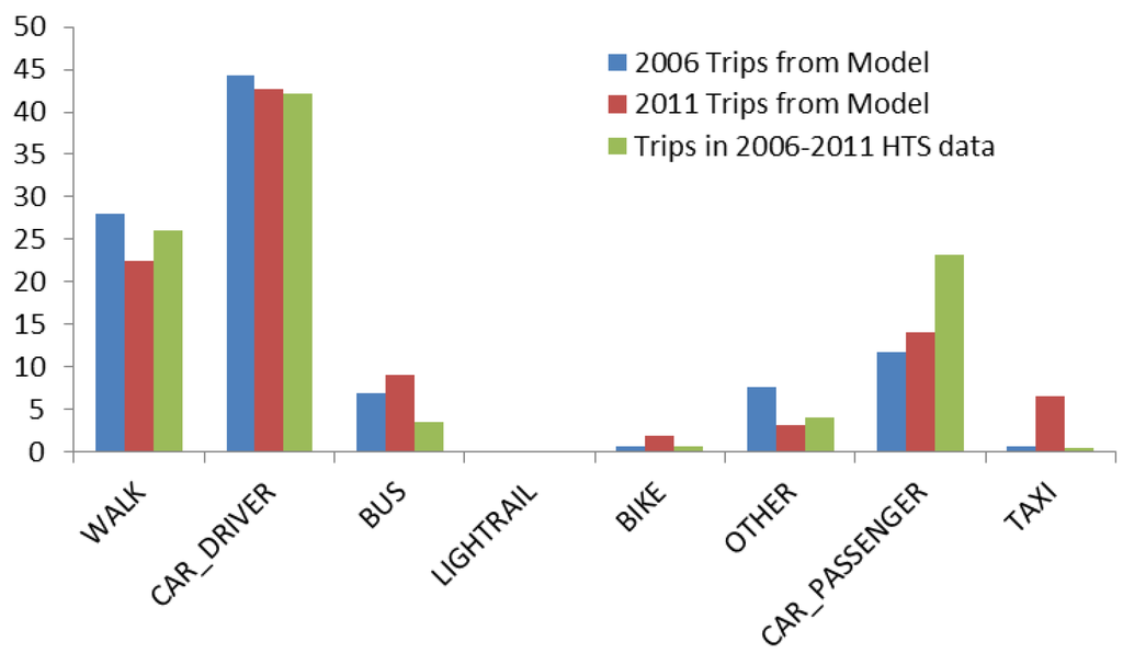
Figure 8.
Percentage of trips by modes from simulation years 2006 and 2011 versus 2006–2011 HTS data.
Figure 8.
Percentage of trips by modes from simulation years 2006 and 2011 versus 2006–2011 HTS data.

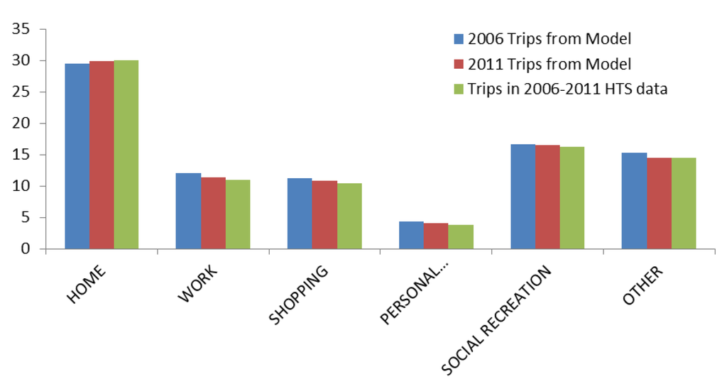
Figure 9.
Percentage of trips by purposes from simulation years 2006 and 2011 versus 2006–2011 HTS data.
Figure 9.
Percentage of trips by purposes from simulation years 2006 and 2011 versus 2006–2011 HTS data.


Figure 10.
Percentage of population by number of daily trips for simulation years 2006 and 2011 versus 2006–2011 HTS data.
Figure 10.
Percentage of population by number of daily trips for simulation years 2006 and 2011 versus 2006–2011 HTS data.
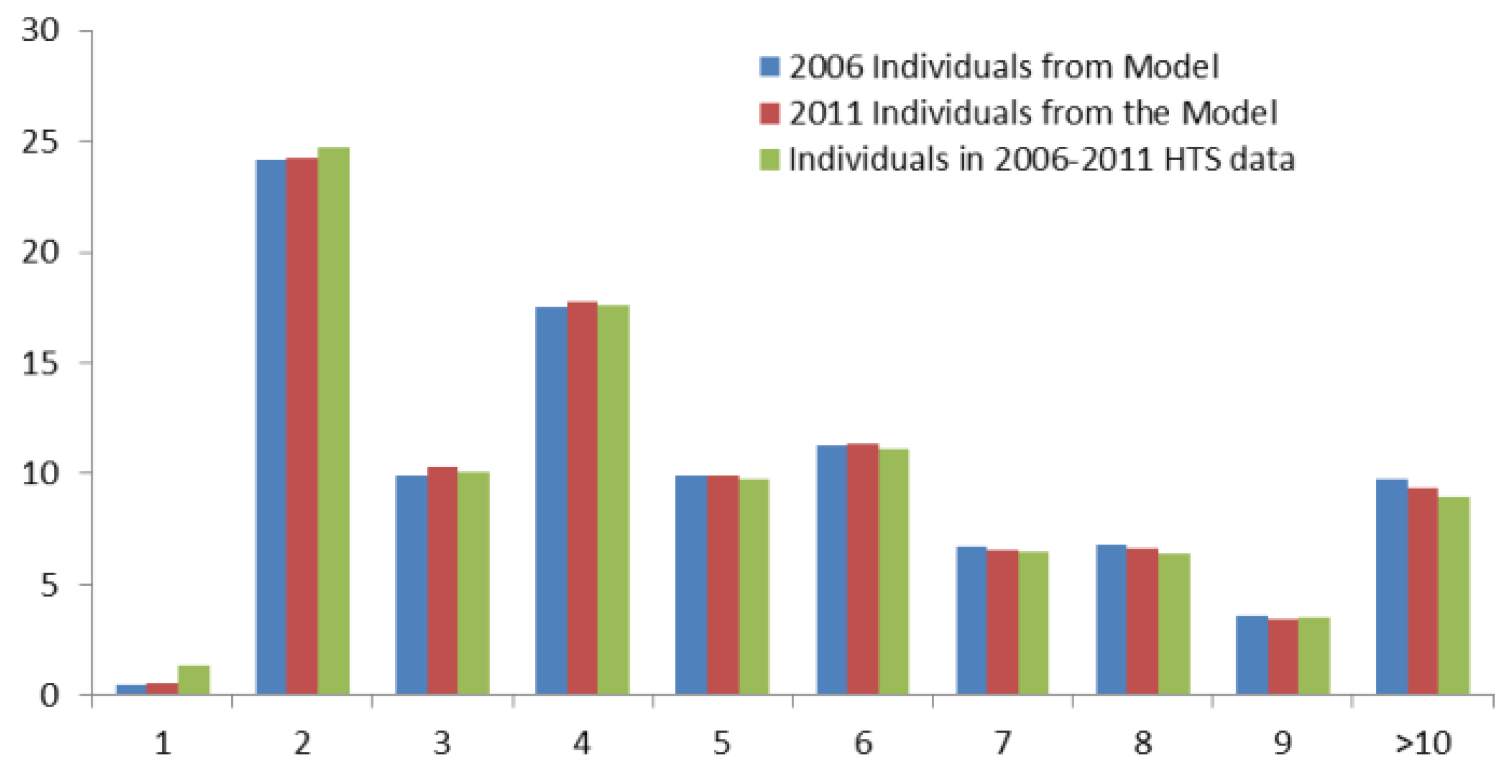
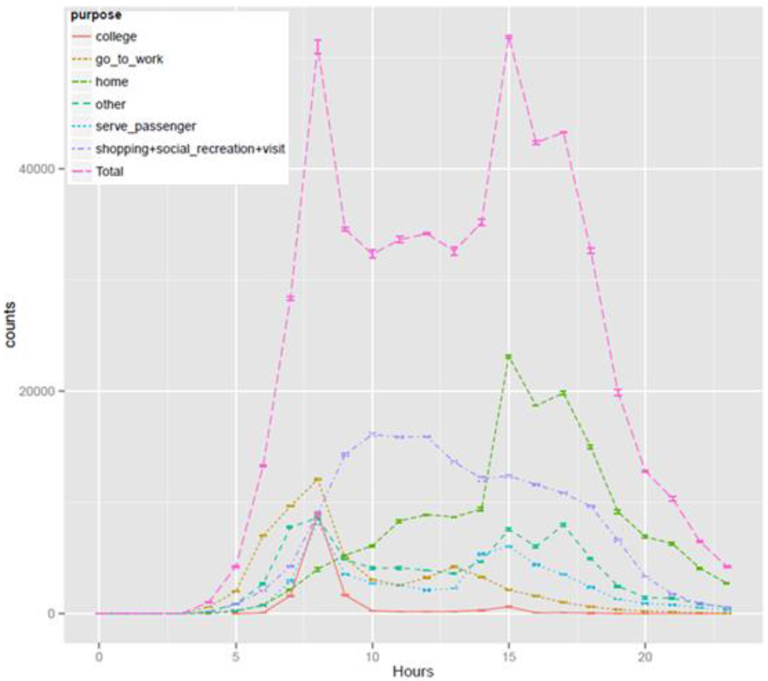
Figure 11 presents trip counts by trip purposes over 24 h of a representative day in year 2011. TransMob not only satisfactorily reproduces the peak of trips to work and trips to school between 8.00 am and 9.00 am; it shows that the count of work trips is higher than that of school strips at earlier hours (6.00 am–8.00 am), which reflects early workers. Trips to work also have a smaller peak between 1.00 pm and 2.00 pm to reflect afternoon and/or night shifts. Trips for shopping, social activities, recreational and personal services reach their peak at around 9.00 am to 12.00 midday and gradually drop in the afternoon. These observations affirm that TransMob can generate plausible patterns of travel demand of the population in the study area as well as the change of these patterns as the population evolves.

Figure 11.
Trip counts by purposes over 24 h of a representative day in year 2011.
Figure 11.
Trip counts by purposes over 24 h of a representative day in year 2011.
3.4. Validation of Road Traffic Density
Traffic density from the behavioural dynamic traffic assignment model (described in Section 2.4) on road links around the University of New South Wales at 8:00am are compared against the corresponding congestion real-world profiles from Google Traffic [36], as shown in Figure 12. The novel micro-traffic simulator incorporated into TransMob is able to reproduce relatively accurately the observed congestion patterns from Google Traffic. Figure 13 shows that the simulated congestion level of every road link on the road network in the study area at 8.00 am, which highlights Anzac Parade (the major artery running across the area) as the most congested, agreeing with the observed traffic in real life. However such agreements do not occur on all parts of the road network. This can be due to missing data from Google Traffic (or Google’s sources) and/or the assumptions of the traffic model as a closed system (i.e., no through traffic in the study area). Another source of discrepancies comes from the randomness in assigning a location to the destination of trips in the travel diary of the synthetic population. While the assignment of a destination location to work related trips is constrained by Journey to Work data, the randomness in assigning destination locations to trips of other purposes does not guarantee a realistic representation of traffic profiles in the model. Note that non-work trips have a significant proportion in the total number of trips made by the population in the study area (see Figure 9 and Figure 11).

Figure 12.
Traffic density around the University of New South Wales at 8.00 am. (a) From the behavioural traffic micro-simulator; (b) From Google Traffic.
Figure 12.
Traffic density around the University of New South Wales at 8.00 am. (a) From the behavioural traffic micro-simulator; (b) From Google Traffic.
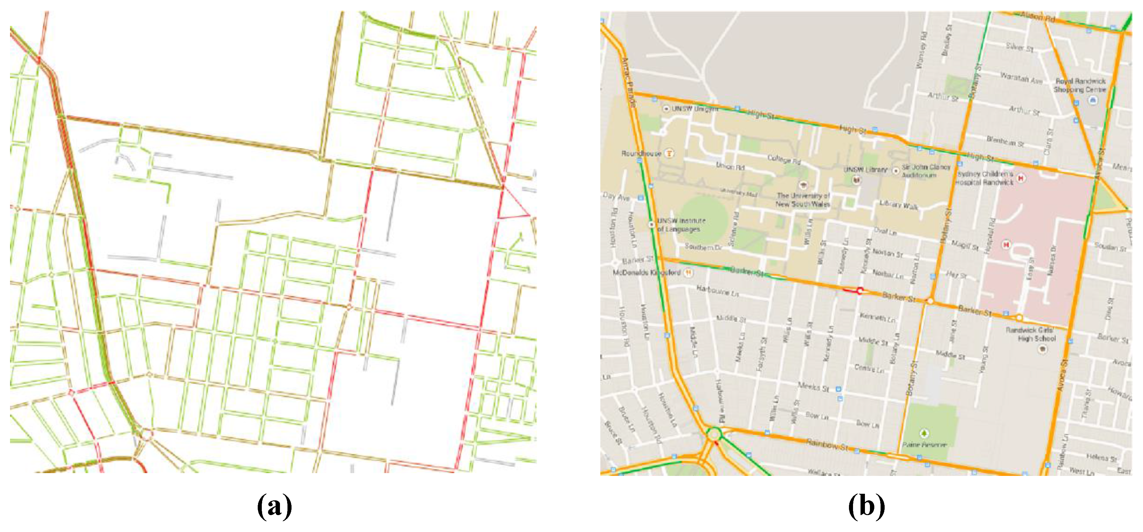
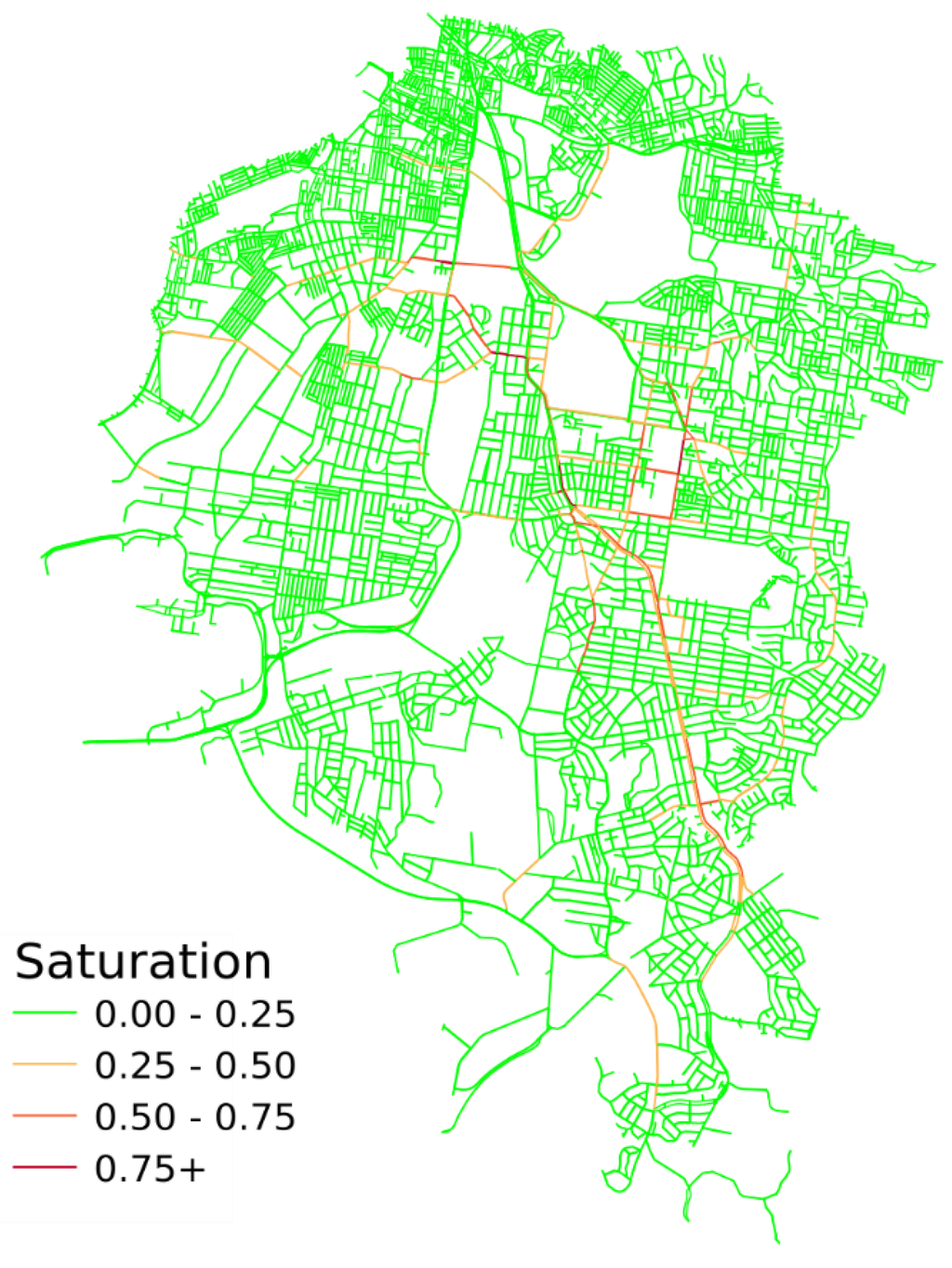
Figure 13.
Saturation of road network in the study area at 8.00 am.
Figure 13.
Saturation of road network in the study area at 8.00 am.

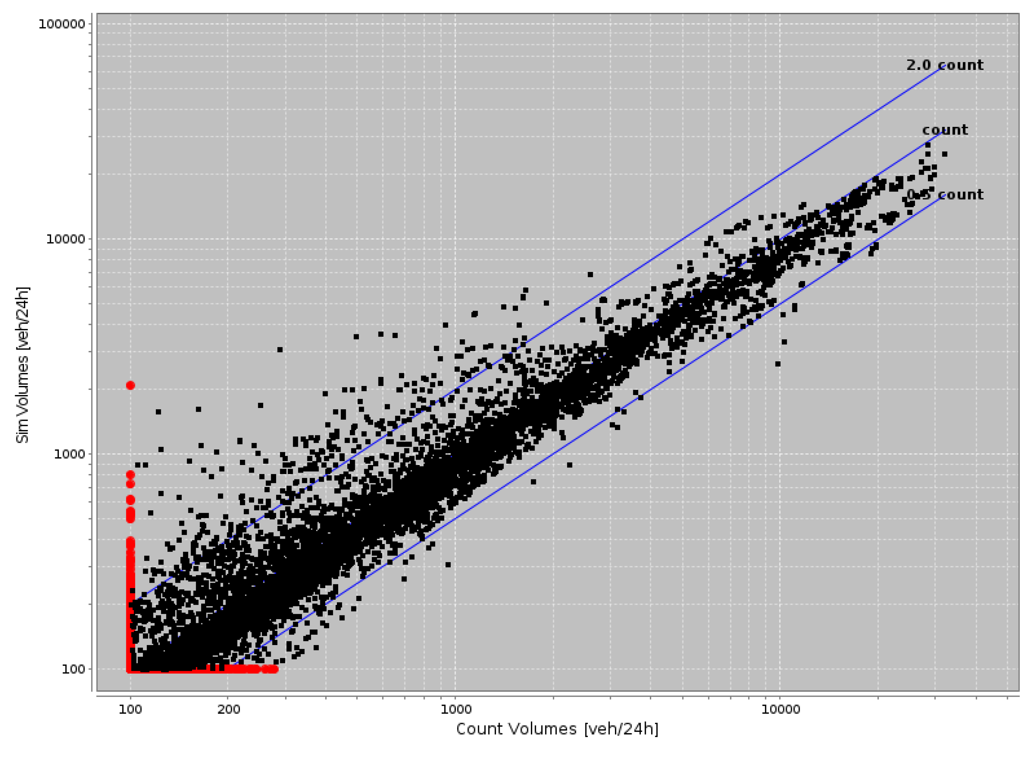
In order to benchmark the novel behavioural dynamic traffic assignment model against a traditional and widely recognised traffic micro-simulator, the results from the novel simulator are compared against the outputs from MATSim using the same set of inputs of travel demands and road network. In Figure 14, the traffic counts over the full simulation period (24 h) from the behavioural dynamic traffic assignment model and from MATSim are represented by the horizontal axis and the vertical axis, respectively. Each data point in the figure represents the traffic counts from our new traffic model and from MATSim for a road link. The strong positive correlation between the counts as observed in the figure (Pearson correlation coefficient of 0.905) indicates that our new traffic model produces traffic patterns similar to those from MATSim. This is an encouraging outcome for a work-in-progress traffic micro-simulator, particularly in considering that it originates from agent-based modelling paradigm that allows for emergent behaviours of vehicle drivers, including dynamic rerouting during the simulation.

Figure 14.
Benchmarking the behavioural traffic micro-simulator against MATSim.
Figure 14.
Benchmarking the behavioural traffic micro-simulator against MATSim.
4. Results and Discussion
The previous section has presented the comparisons of TransMob results against various survey data in a bid to validate its capability in satisfactorily reproducing the observed complexity of the dynamics of the selected urban area. The current section will demonstrate the application of TransMob for exploratory study of emergent behaviours of an urban area via a number of hypothetical scenarios of planning policies. The simulation period is 20 years for all scenarios starting in 2006. Details of the simulated scenarios are as follows
- -
- Scenario 1 (base line): This is the continuing of the validation simulation (for 5 years) presented in Section 3 for 15 more years into the future.
- -
- Scenario 2: Unlimited supply of dwelling stocks in the study area over the simulation period.
- -
- Scenario 3: An enhanced proportion of a Double Income No Kids (DINK) population.
- -
- Scenario 4: Introduction of a light rail corridor into the study area and unlimited supply of dwelling stocks in travel zones along the light rail corridor.
The above scenarios are selected to give comparative understanding of the model outcomes that can be generated from the use of a scenario exploration approach. More importantly they aim at demonstrating the capability of TransMob to properly react to various inputs. The assumptions made in these illustrative scenarios, therefore, are drastic in order to introduce extreme conditions in the model inputs. The remaining of this section describes inputs into TransMob for each scenario (compared to the base line scenario) and their simulation outputs. The results of the runs for each scenario did not vary in a significant way (intra-scenario) and for clarity we only illustrate one run.
4.1. Scenario 1—Base Line
The simulation in this scenario is the continuation of validation simulation presented in Section 3 for a total simulation time of 20 years. At the end of the simulation, the population in the area increases by 18% to almost 126,000 individuals and over 58,000 households. Factors affecting the population growth include the net immigration, the availability and pricing of dwelling stocks, and the evolution rates used in evolving the population.
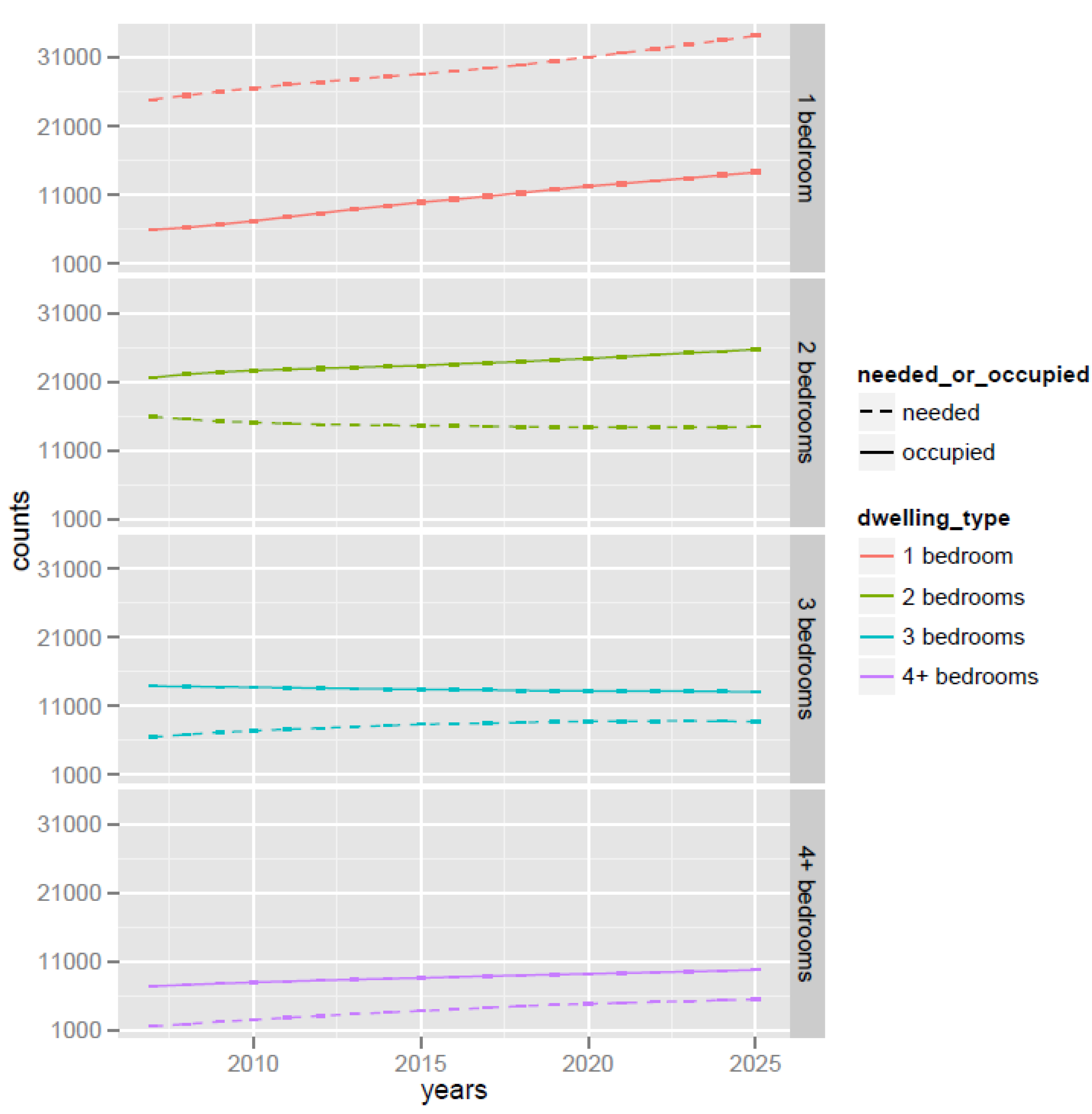
The change in the number of occupied dwellings by size over the course of the simulation is shown in Figure 15. Dotted lines represent the demand of dwellings of a particular size calculated based on the number of adults (over 15 years old), whether they are a couple, and the number of children in the household. Solid lines represent the dwellings actually occupied by households in the population. These two lines are not necessarily close to each other because the relocation algorithm allows a household to move into a dwelling one bedroom larger than its needs if the household can afford it (see Section 2.6). This feature is better illustrated in Table 2, which details of the number of dwellings needed by households in the synthetic population and the number of dwellings actually occupied by these households at the end of the simulation.

Figure 15.
Change of number of dwellings by size over simulation period for base line scenario.
Figure 15.
Change of number of dwellings by size over simulation period for base line scenario.
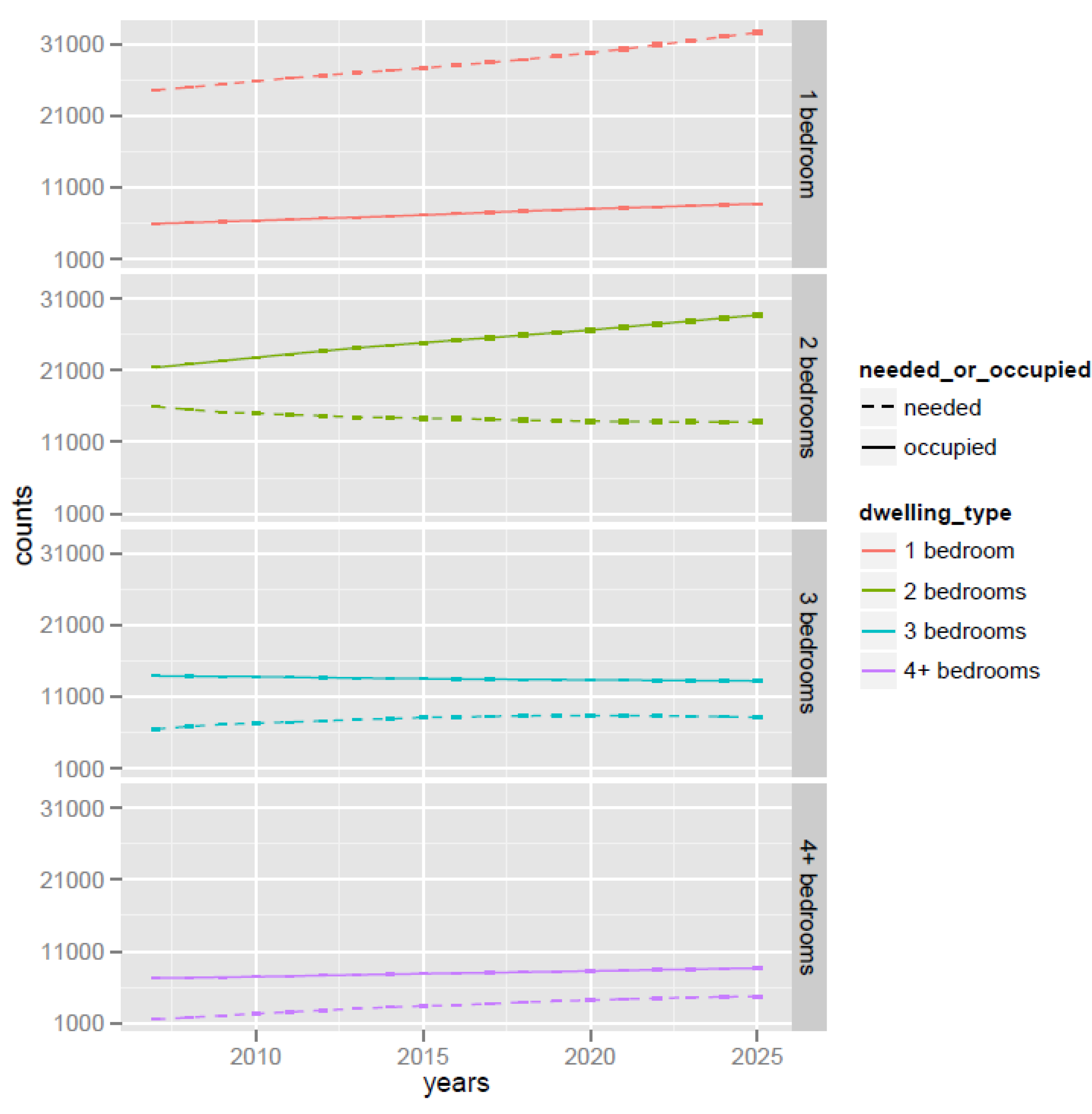
Table 2.
Comparison of number of dwellings needed and number of dwellings actually occupied by synthetic households in year 2026 for base line scenario.
| Types of Dwellings | Dwellings Needed (Based on Composition of Residents of Households in the Population) | Dwellings Occupied | Households Searching for Dwellings with 1 Bedroom Larger Than Needed | Dwelling Stocks |
|---|---|---|---|---|
| 1 bedroom | 32,072 | 8557 | 23,515 | 11,451 |
| 2 bedrooms | 13,490 | 28,086 | 8919 | 30,981 |
| 3 bedrooms | 7958 | 13,028 | 3849 | 18,159 |
| 4 bedrooms or more | 4752 | 8601 | 0 | 12,852 |
At the end of the simulation (year 2026), only 8557 out of 32,072 households that need one bedroom actually live in one-bedroom dwellings. The remaining 23,515 households search for, and eventually live in, two-bedroom dwellings. This means that out of 13,490 households that need two bedrooms, only 4571 of them live in two-bedroom dwellings. There are 8919 of these households searching for and eventually living in three-bedroom dwellings. Note that this is not a result of the unavailability of two-bedroom dwelling stocks because there are almost 3000 (30,981 minus 28,086) dwellings of this type remain unoccupied. Instead, these 8919 households end up live in three-bedroom dwellings, which can be explained by the mechanism described in Section 2.6. Specifically, these households (i) prefer living in a travel zone with higher liveability index and (ii) can afford a dwelling larger than their needs. The same explanation applies to households living in larger dwellings (with three bedrooms or more), i.e., out of 7958 households that need three bedrooms, only 4109 of them end up residing in three-bedroom dwellings. The remaining (3849 households), together with 4752 households that actually need four bedrooms or more, live in 8601 dwellings having more than three bedrooms.
The average satisfaction of the population in three age groups for each travel zone is plotted in Figure 16. Note that as only people over 15 years old were interviewed in the liveability survey, TransMob is able to calculate liveability and satisfaction index only for individuals over 15 years of age in the simulation. As Figure 16 shows, the majority of the population in all travel zones in the study area are between 30 and 64 years old, while younger group of people (15–29) and older group of people have approximately equal proportions. People above 65 years old appear to be more satisfied with their travel zones compared to people between 30 and 64 years old, who in turn, appear to be more satisfied with the people in the youngest age group. This is further illustrated in the histograms of average satisfaction of these three age groups in Figure 17.
With regards to transport demands, the distribution of trips over 24 h of a simulated day by trip purposes resembles that in Figure 11. The total number of trips however is higher due to a higher population in year 2026 compared to 2011. It is worth noting that trips that are declared as work related and going to school occupy totally only around 34% the total number of trips made in the morning peak hours. Even if we assume that the majority of trips marked as “serve passengers” are for dropping off children at school or people at work, over 50% of trips made in peak hours of a weekday are not work/school related. Driving drops from approximately 47% of mode share in 2006 to 40% in 2026 but remains the most popular/preferred transport mode, followed by walking (23%), car passengers (13%), and bus (9%).

Figure 16.
Average satisfaction versus proportion of three age groups in the population for base line scenario.
Figure 16.
Average satisfaction versus proportion of three age groups in the population for base line scenario.
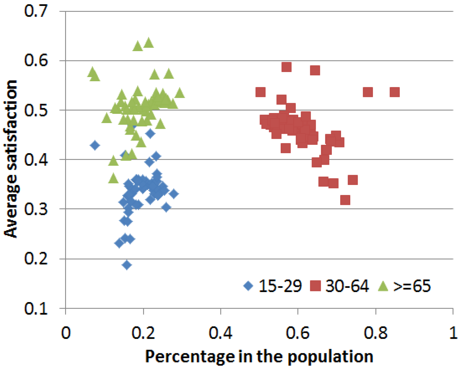
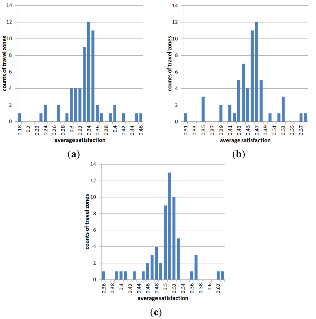
Figure 17.
Histograms of average satisfaction of three age groups in the population for base line scenario. (a) Age group 15–29; (b) Age group 30–64; (c) Age group ≥65.
Figure 17.
Histograms of average satisfaction of three age groups in the population for base line scenario. (a) Age group 15–29; (b) Age group 30–64; (c) Age group ≥65.

4.2. Scenario 2—Unlimited Supply of Dwelling Stocks
The inputs into this scenario are similar to those for Scenario 1 (base line scenario), except that the supply of dwelling stocks is abundant throughout the simulation period (2006–2026) across the whole study area. Thanks to this change in inputs, households have more chance to find a suitable dwelling and thus do not have to relocate to outside of the study area. This results in a higher population growth in this scenario compared to Scenario 1. The total population reaches 134,445 people and 61,751 households in 2026 in this scenario. Change of number of dwellings by size over the simulation period is shown in Figure 18. Note that the demand for dwellings in Scenario 2 is similar (in terms of the quantity in each year and the growth rate across the years) to the demand for dwellings in Scenario 1 across all dwelling types. However, the gap between the numbers of needed dwellings (i.e., the dotted line) and the numbers of occupied dwellings (i.e., the solid line) for one-bedroom dwellings and two-bedroom dwellings (the top two graphs in Figure 18) are significantly smaller than those in Scenario 1. However these gaps for three-bedroom dwellings or larger (the bottom two graphs in Figure 18) remain very similar to those in Scenario 1. An explanation to these observations is given below.
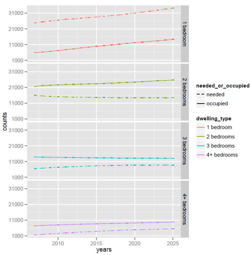
Figure 18.
Change of number of dwellings by size over simulation period for Scenario 2.
Figure 18.
Change of number of dwellings by size over simulation period for Scenario 2.
As aforementioned, thanks to the unlimited supply of dwelling stocks while the distributions of household income and distributions of house price are unchanged, more households who search for small dwellings (having less than three bedrooms) could successfully find one as opposed to Scenario 1, in which affordable dwellings would be very quickly run out of stock. This explains the smaller gap between the number of dwellings searched for and number of dwellings actually occupied in Scenario 2 compared to Scenario 1 for one- and two-bedroom dwellings. Meanwhile, households who search for larger dwellings, while not facing the problem of limited stocks, may still have to face the higher price tags of these dwellings (compared to their budget and income) as they would in Scenario 1. Thus in Scenario 2, it is equally financially difficult for large households to find a suitable dwelling compared to Scenario 1, which explains the same gaps between the number of dwellings searched for and number of dwellings actually occupied compared to Scenario 1 for dwellings with three bedrooms or more.
It is also noted that “occupied” one-bedroom dwellings remain below “needed” one-bedroom dwellings even though the supply of dwellings is unlimited in this scenario. An explanation is that the search for a relocating dwelling is constrained by both availability and affordability (and liveability). More specifically, a household searches into most liveable travel zone(s) first for a suitable dwelling, which for the current case has either one bedroom or two bedrooms. Please note that only if they cannot find any affordable dwellings that they move to the next (and less liveable) travel zone(s). Thanks to the unlimited dwelling stocks, there is always something available in a particular travel zone. The household however may not afford a one-bedroom dwelling but can afford a two- bedroom dwelling. Furthermore, if it can afford either a one-bedroom or a two-bedroom dwelling, the algorithm randomly selects one of the two options.
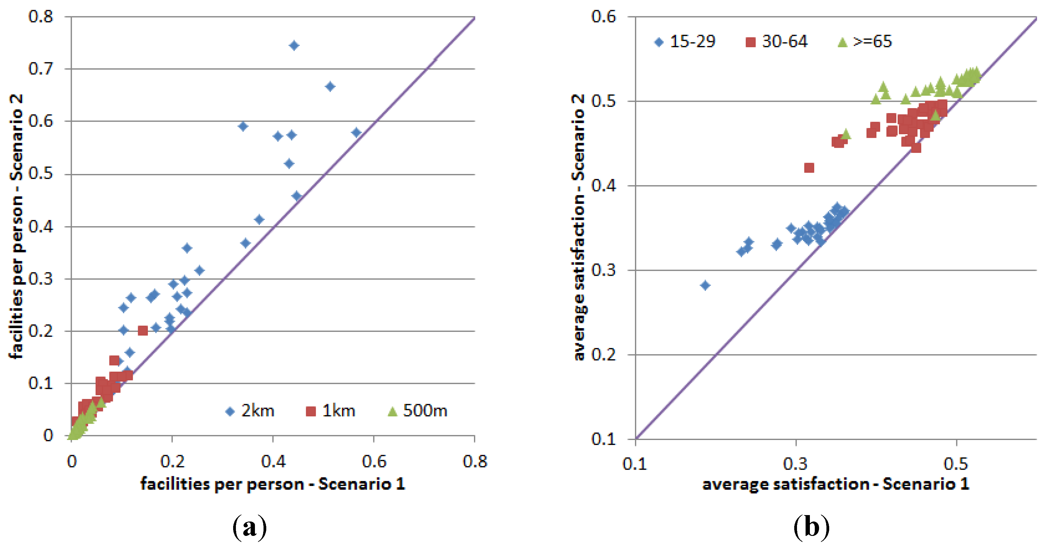
As the choice of a relocating travel zone in Scenario 2 is less constrained, some travel zones will end up having higher population (and some lower) compared to Scenario 1. Because the number of facilities and services available in each travel zone is the same between the two scenarios, residents in travel zones with higher population will have a lower access to the facilities and services, leading to a drop of satisfaction perception in these travel zones as compared to Scenario 1. This is because the value of average facilities (number of facilities and services accessible by a person) of a travel zone is an influential attribute in the calculation of satisfaction index of a person [19,20]. This relationship between average facilities of a travel zone and the average satisfaction of the population in the travel zone is illustrated in Figure 19 and Figure 20. These figures compare the number of facilities and services per capita in travel zones in Scenario 2 versus Scenario 1 and the corresponding average satisfaction of residents in the travel zones. Three ranges of average facilities for a travel zone are presented, within 500 m, 1 km, and 2 km radii of the centroid of the travel zone. The average satisfaction is presented for three groups of people, young (under 30), middle age (between 30 and 64), and elderly (above 65).
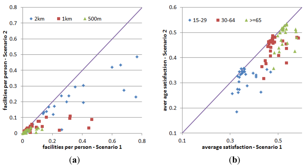
Figure 19.
Average satisfaction of travel zones in Scenario 2 having lower average facilities compared to Scenario 1. (a) Average facilities within three radii from travel zone centroid; (b) Average satisfaction of three age groups.
Figure 19.
Average satisfaction of travel zones in Scenario 2 having lower average facilities compared to Scenario 1. (a) Average facilities within three radii from travel zone centroid; (b) Average satisfaction of three age groups.
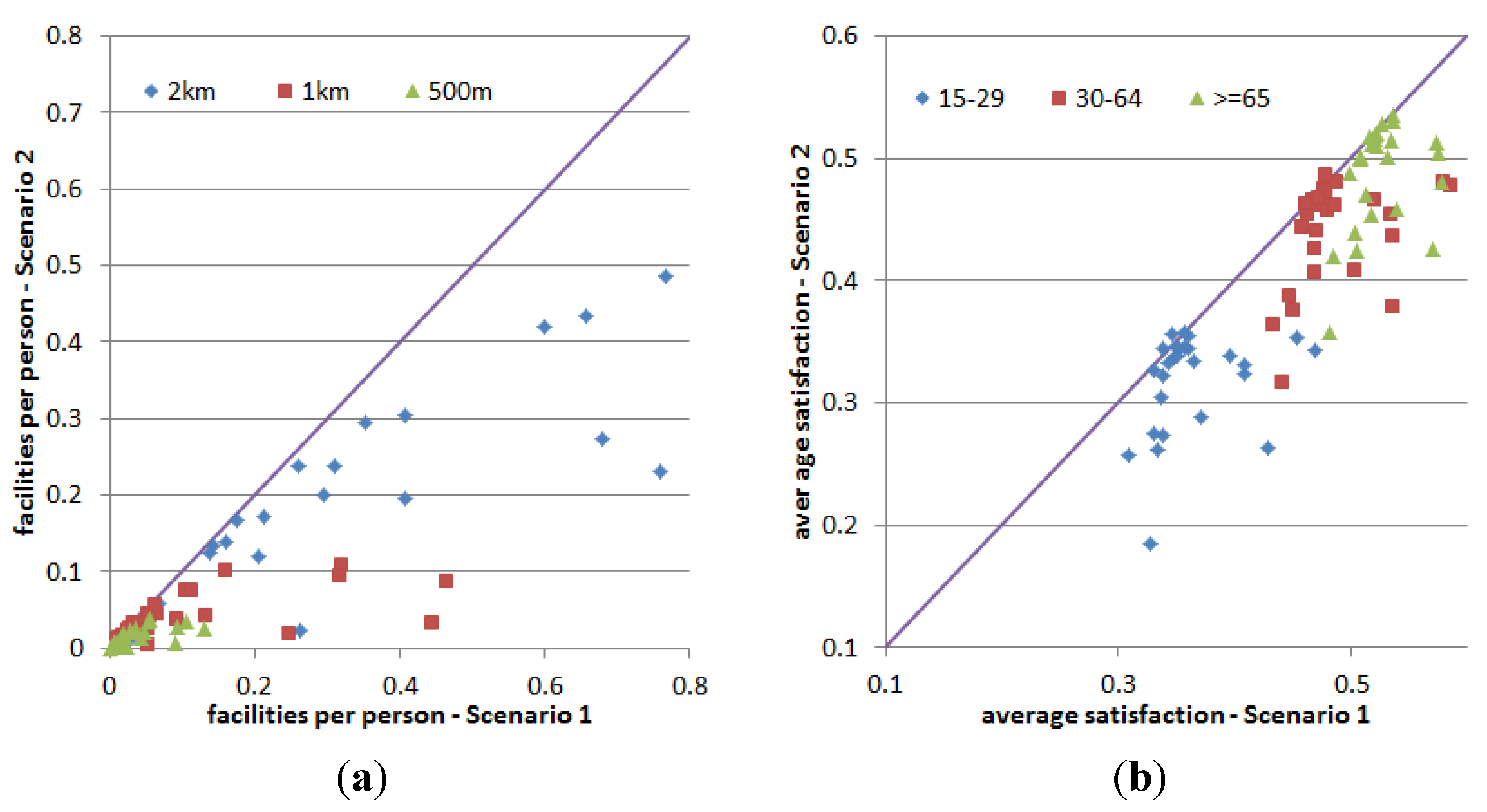
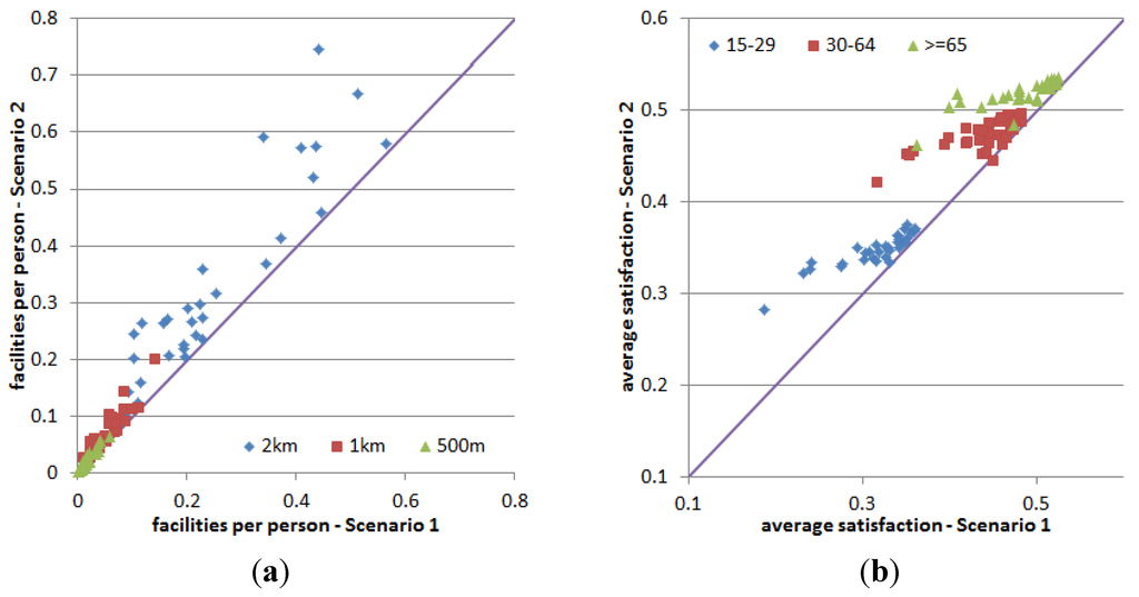
Figure 20.
Average satisfaction of travel zones in Scenario 2 having higher average facilities compared to Scenario 1. (a) Average facilities within three radii from travel zone centroid; (b) Average satisfaction of three age groups.
Figure 20.
Average satisfaction of travel zones in Scenario 2 having higher average facilities compared to Scenario 1. (a) Average facilities within three radii from travel zone centroid; (b) Average satisfaction of three age groups.
With regards to transport profiles, the composition of trips made by the population by modes and by trip purposes in Scenario 2 resembles that from Scenario 1. This is because there are no changes in the demographics composition of the population between the two scenarios. The total number of trips however is larger (by 6.7%) in Scenario 2 than in Scenario 1, which reflects the higher transport demands of a larger population in this scenario.
4.3. Scenario 3—Double Income No Kids Households
In this scenario, we model the case when the proportion of Double Income No Kids (DINK) households in the study area is increased rapidly over the simulated years. This is achieved by doubling the rates of marriage, halve the birth rate across all female ages, and halve the divorcing rates. The remaining of the inputs into this scenario is similar to those in Scenario 1.
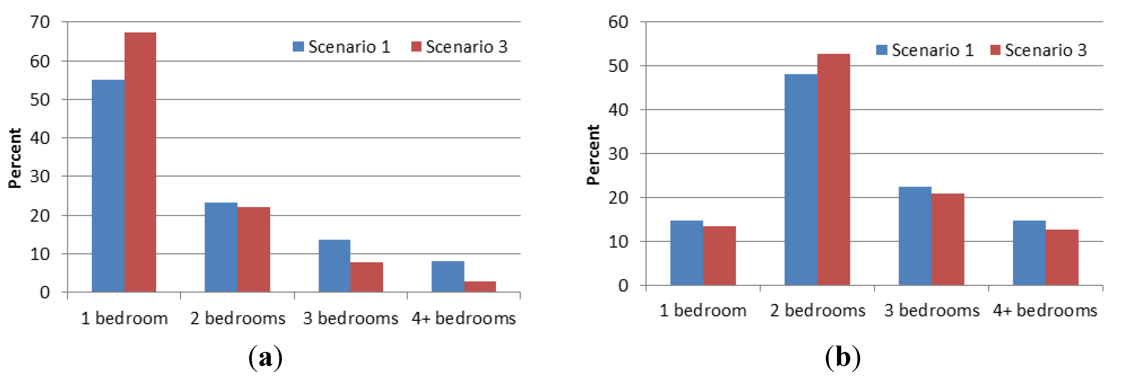
Thanks to these changes in inputs, the population growth in Scenario 3 is slower compared to Scenario 1. The final population is only 7.1% higher than the initial population, as compared to over 18% in Scenario 1. The average household size in the population at the end of the simulation in Scenario 3 is also smaller, at two persons per household compared to 2.16 persons per household in Scenario 1. A direct result of this is that the demand for small dwellings (e.g., having one bedroom) is significant higher in Scenario 3 as compared to Scenario 1, and vice versa for large dwellings (having three bedrooms or more), as evidenced in Figure 21.

Figure 21.
Comparing the proportion of dwellings by size as needed and occupied by households in Scenarios 1 and 3 in year 2026. (a) Needed dwellings; (b) Occupied dwellings.
Figure 21.
Comparing the proportion of dwellings by size as needed and occupied by households in Scenarios 1 and 3 in year 2026. (a) Needed dwellings; (b) Occupied dwellings.
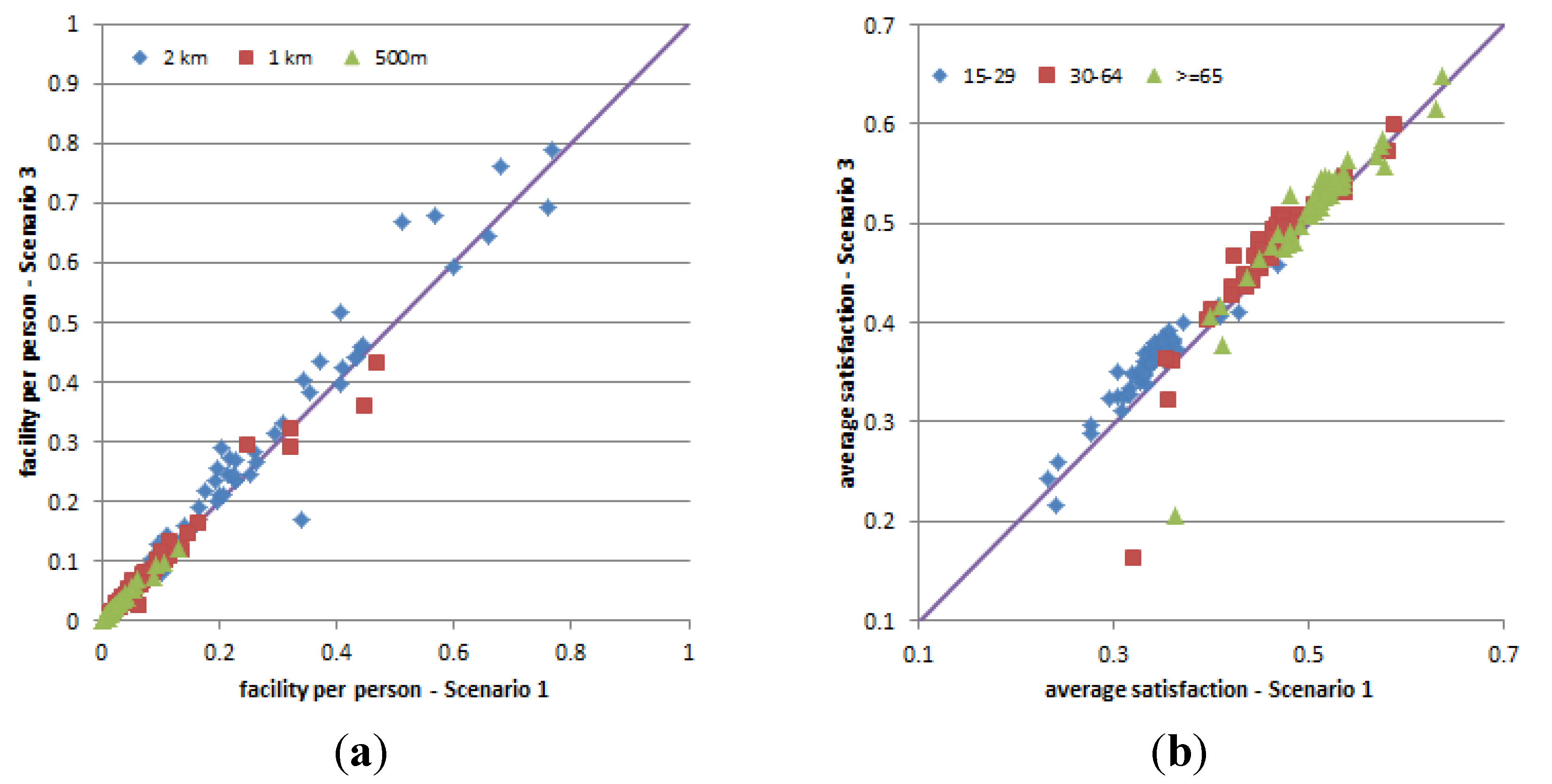
Another effect of lower birth rates to the population structure in this scenario is primarily in the lower number of children under 15 years old at the end of the simulation compared to Scenario 1. The number of people between 15 and 29 years of age is also slightly smaller than that in Scenario 1. This is because in Scenario 3, there are fewer babies born in the first five years of the simulation compared to Scenario 1, who will reach the age of 15 (and older) after 20 years. There would not be a very big difference in the proportion of people in older age groups in the population in this scenario compared to Scenario 1 (which would be the case had the death rates were increased). This is evidenced in Figure 22, which compares proportions of the population in three age groups in Scenario 3 against those in Scenario 1. Because of this, the average facilities (number of facilities available to a person over 15 years old) in this scenario is not so different to that in Scenario 1 in the majority of the travel zones, as evidenced in Figure 23a, leading to very similar the average satisfaction for people over 15 years old between the two scenarios across all travel zones (Figure 23b).

Figure 22.
Comparing proportion of population in three age groups in Scenario 3 against Scenario 1.
Figure 22.
Comparing proportion of population in three age groups in Scenario 3 against Scenario 1.
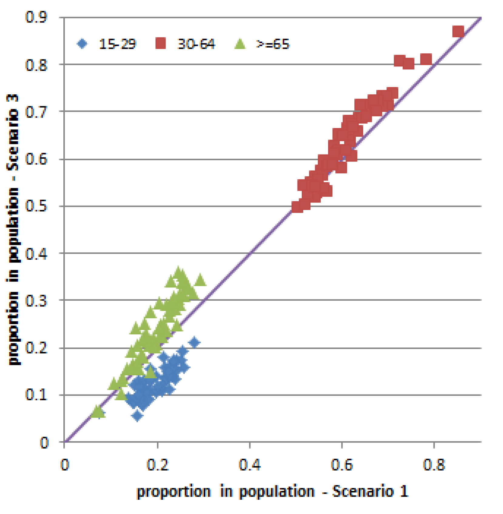

Figure 23.
Comparison of average facilities and average satisfaction of travel zones in Scenario 3 against Scenario 1. (a) Average facilities within the three radii (500 m, 1 km, and 2 km) from travel zone centroid; (b) Average satisfaction of three age groups (15–29, 30–64 and 65+).
Figure 23.
Comparison of average facilities and average satisfaction of travel zones in Scenario 3 against Scenario 1. (a) Average facilities within the three radii (500 m, 1 km, and 2 km) from travel zone centroid; (b) Average satisfaction of three age groups (15–29, 30–64 and 65+).
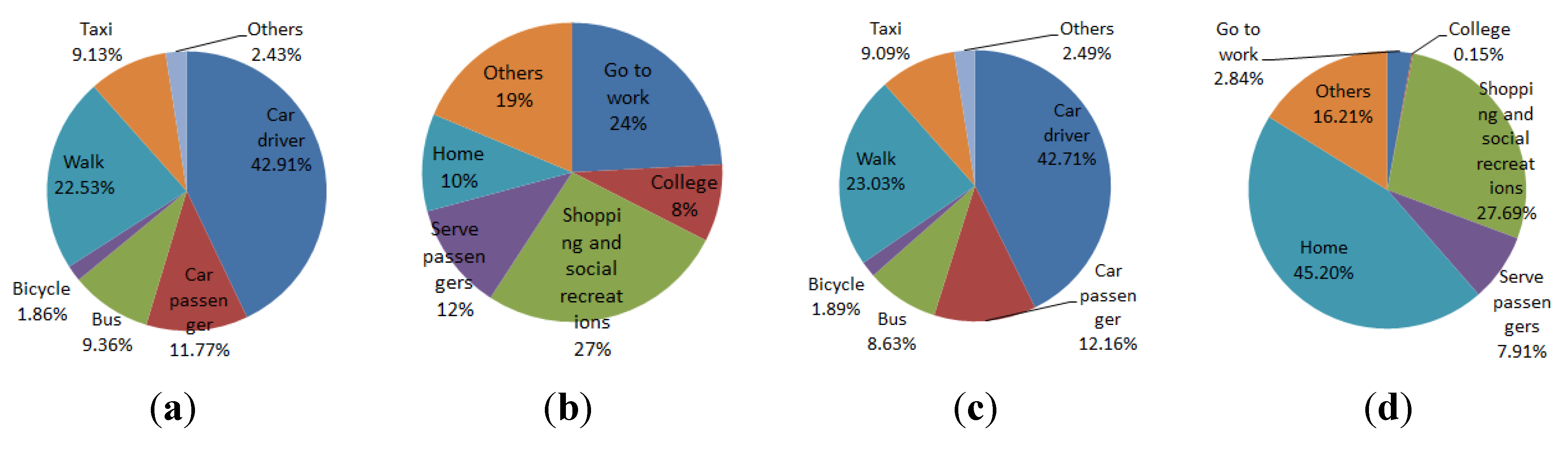
With regards to transport, the total number of trips made in a representative day in 2026 is less than that in Scenario 1, reflecting the smaller demands of a smaller population. More interestingly, the composition of the trips exhibits some noticeable differences between the two scenarios (see Figure 24 and Figure 25). Because there are less children under 15 in Scenario 3 at the end of the simulation, the percentage of trips to university/schools drops in the morning peak hours (between 7.00 am and 10.00 am) from 11.78% in Scenario 1 to around 8% in Scenario 3. The percentage of trips to serve passengers, which are composed considerably by trips for picking up and dropping off children at schools, is also lower in Scenario 3 for both the morning and afternoon peak hours. The effects of having less children in the population are also reflected in mode shares, with a drop in the percentage of car passengers in Scenario 3 for both the morning and afternoon peak hours (Figure 25a,c). A higher proportion of car drivers in Scenario 3 could be attributed to the fact that there are more adults/elderly people in the population of this scenario.

Figure 24.
Percentage of trips by modes and by purposes in AM and PM peak hours in Scenario 1 in year 2026. (a) Trips by modes AM; (b) Trips by purposes AM; (c) Trips by modes PM; (d) Trips by purposes PM.
Figure 24.
Percentage of trips by modes and by purposes in AM and PM peak hours in Scenario 1 in year 2026. (a) Trips by modes AM; (b) Trips by purposes AM; (c) Trips by modes PM; (d) Trips by purposes PM.
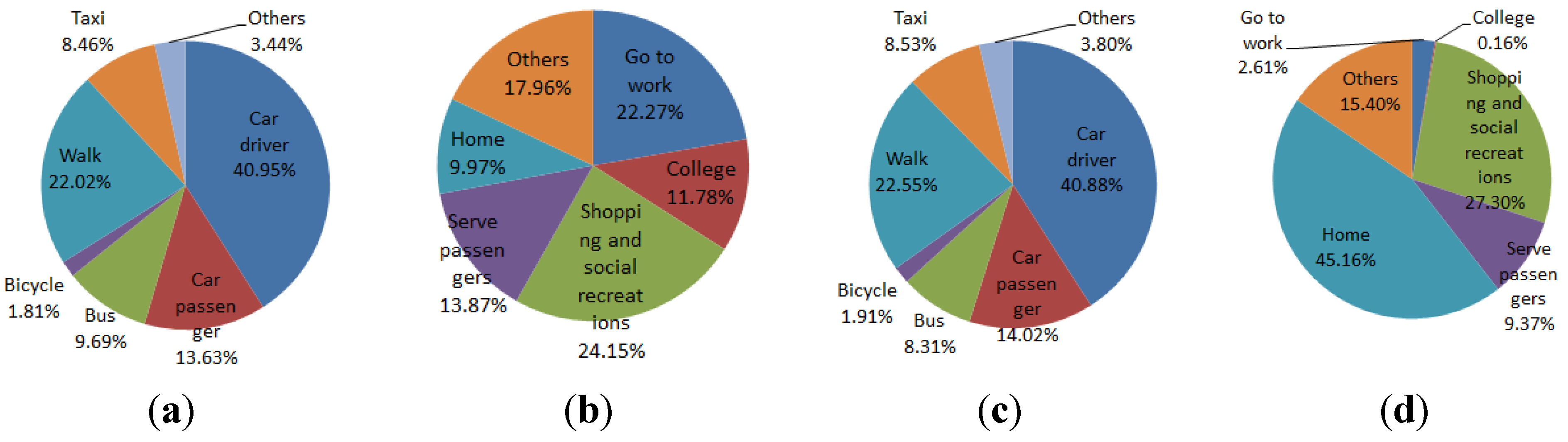

Figure 25.
Percentage of trips by modes and by purposes in AM and PM peak hours in Scenario 3 in year 2026. (a) Trips by modes AM; (b) Trips by purposes AM; (c) Trips by modes PM; (d) Trips by purposes PM.
Figure 25.
Percentage of trips by modes and by purposes in AM and PM peak hours in Scenario 3 in year 2026. (a) Trips by modes AM; (b) Trips by purposes AM; (c) Trips by modes PM; (d) Trips by purposes PM.
4.4. Scenario 4—New Light Rail Corridor with Population Densification along the Corridor
This scenario investigates a proposed light rail line to the main campus of the University of New South Wales located in the study area. However, it should be noted that this work is illustrative only and does not form part of, or validate, any economic evaluations of options of infrastructure development that may be undertaken by the Government. A map of the simulated light rail corridor and the surrounding travel zones is shown in Figure 26. It is assumed in Scenario 4 that light rail is available at full capacity from the 1st simulated year, and that light rail services depart every 5 min for all of a 24 h day, at a capacity of 104 passengers per light rail vehicle. In order to reproduce the impacts of the new light rail corridor to housing developments, the supply of housing stocks is assumed unlimited, i.e., housing availability in this subarea is completely demand driven. Finally, the immigrating population is assumed three times higher than that in Scenario 1.
The population growth in Scenario 4 is highest among the scenarios examined, reaching almost 155,000 individuals and over 69,000 households at the end of the simulation. This is primarily due to the large amount of immigrants introduced into the population at every simulated year, as well as the unlimited supply of dwelling stocks along the light rail corridor, which helps retain more population inside the study area. This is further evidenced by the results in Table 3, which show that for travel zones along the corridor at the end of the simulation, the number of occupied dwellings in Scenario 4 is much higher as compared to Scenario 1 across all dwelling sizes. Similar to the discussion of results of average satisfaction in Scenario 2, a higher density of population along the light rail corridor leads directly to lower average facilities, and thus a lower average satisfaction of the population in this area. Meanwhile as the population does not change too much across the remaining of the study area, the average facilities and the average satisfaction of the population in travel zones outside the corridor are relatively similar to Scenario 1.
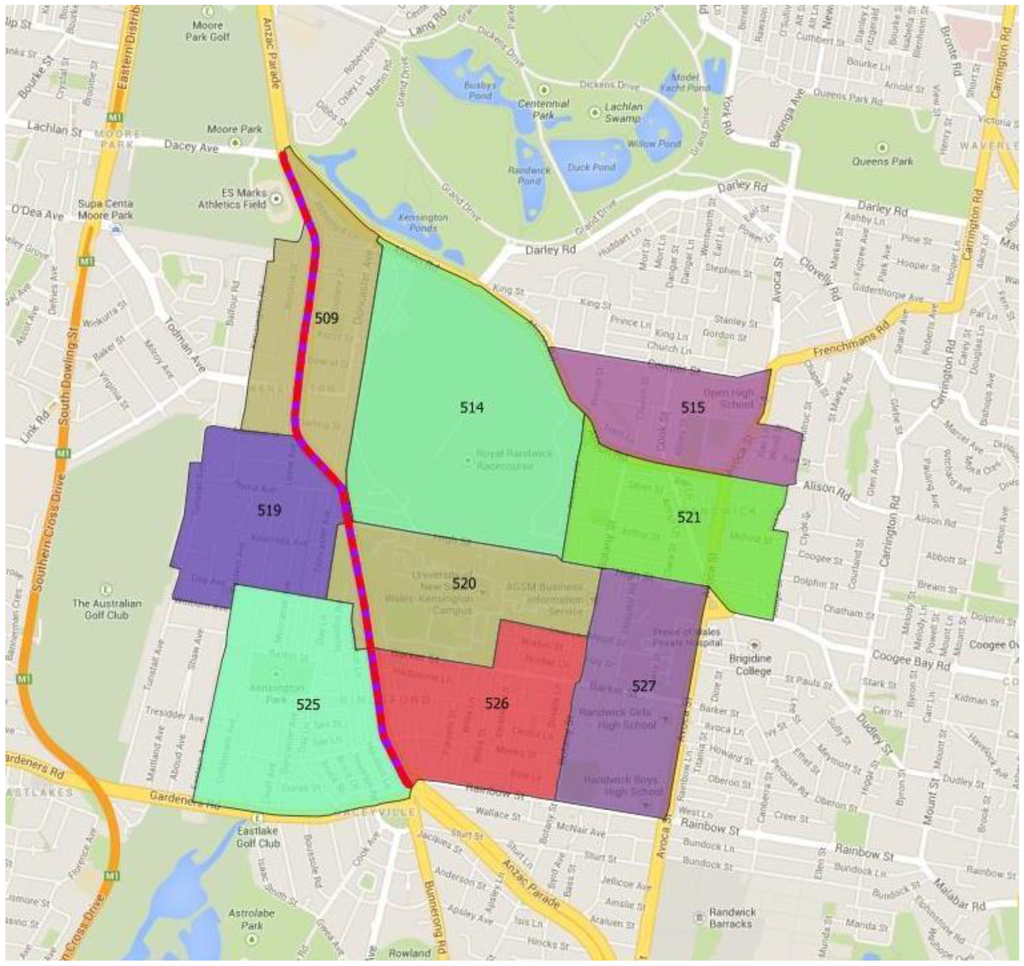
Figure 26.
Travel zones along the simulated light rail corridor.
Figure 26.
Travel zones along the simulated light rail corridor.

Table 3.
Comparing occupied dwellings by sizes in travel zones inside the light rail corridor at the end of the simulation between Scenarios 4 and 1.
| 1 Bedroom | 2 Bedrooms | 3 Bedrooms | ≥4 Bedrooms | |
|---|---|---|---|---|
| Scenario 1 | 1771 | 5556 | 1543 | 682 |
| Scenario 4 | 5928 | 7644 | 2577 | 1248 |
With regards to transport, a major change compared to Scenario 1 is the adoption of light rail as an alternative travel mode. In particular, in the three hours of the morning peak (7.00 am–10.00 am) there are around 4000 light rail trips. The afternoon peak hours see approximately the same amount of light rail traffic. Note that this number of trips is very close to the assumed capacity of the light rail line. With a light rail train departing every 5 min over 24 h of a simulated day and a capacity of 104 passengers each train, there are over 3700 individual passengers that can be carried over a three-hour period from the first station to the end of the line. The number of trips in the morning peak hours and afternoon peak hours from TransMob is slightly larger than the theoretical value of 3700 passengers because an individual passenger can make multiple light rail trips between stations along the light rail line.
Mode shares over the whole simulated day in the final year of the simulation period are shown in Figure 27. The total number of light rail trips over the whole day (around 20,500 trips) is lower than the daily theoretical capacity (29,600 individual passengers) because this capacity is estimated with an assumption of constant passengers boarding the light rail across 24 h of a day, which is unrealistic. Indeed, the demand for light rail follows the travel demand (travel diary) of the population across the day, which only becomes significant between around 5.00 am to around 10.00 pm.
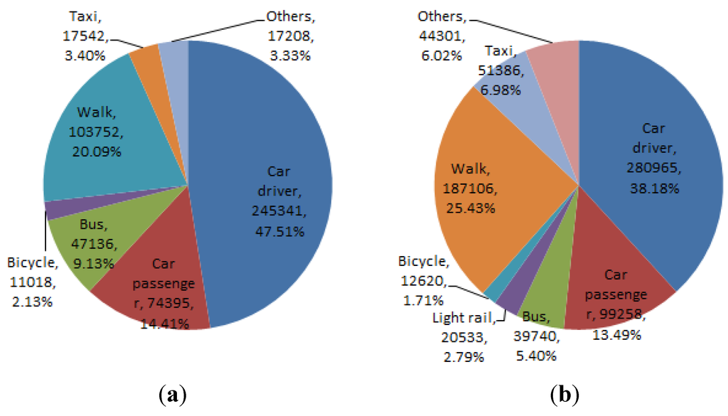
Figure 27.
Mode shares for the whole simulated day for Scenario 4. (a) Initial mode shares; (b) Mode shares at the end of simulation.
Figure 27.
Mode shares for the whole simulated day for Scenario 4. (a) Initial mode shares; (b) Mode shares at the end of simulation.

5. Conclusions
This paper has presented an agent based model, TransMob, for the simulation of the dynamics between demographic evolution, transport demand, housing needs and the eventual change in the liveability perception of the population. The ability to explicitly simulate such dynamics is a unique feature that has not been found in many other agent based models for urban transport and/or urban planning purposes. The model thus is highly suitable for studies exploring long-term consequences of various transport and land use planning scenarios.
TransMob is composed of six major modules, synthetic population, perceived liveability, travel diary assignment, traffic micro-simulator, residential location choice, and travel mode choice. We have reported the application of TransMob to simulate the urban dynamics for Randwick and Green Square, a metropolitan area in south east of Sydney, Australia between from 2006 to 2011 (Section 3). The simulation results in 2011 are vigorously compared against real life survey data available in 2011 across various attributes of the area, including population demographics, housing structures, transport demands, and road traffic density. Satisfactory agreements from these comparisons validate the capability of TransMob in reproducing observed complexity of an urban area.
In a bid to demonstrate the capability of TransMob to properly react to various inputs, we have presented the application of TransMob to simulate hypothetical scenarios of urban planning policies. The assumptions made in these scenarios are quite drastic so that extreme input conditions in various aspects can be introduced to model. These aspects include the availability of residential property (Scenario 2), demographic structure of the population (Scenario 3), public transport options (Scenario 4), and rapid growth of the population (Scenario 4).
Results presented in Section 4 have shown that major modules in the model (i.e., transport, demographic population, satisfaction, residential mobility) are able to response accordingly to these extreme conditions. With unlimited supply of dwelling stocks (in Scenario 2), the TransMob predicts a much larger population residing inside the study area, and higher transport demands in peak hours across all trip purposes and transport modes. It successfully reproduces the reasoning of households in choosing a dwelling to relocate under such a special condition of dwelling stock supply. Given a demographic structure that would result in a higher growth of DINK (double income no kids) households, the model predicts a smaller population (compared to baseline scenario), higher demands for small dwellings (having two bedrooms or less), and a lower number of trips to school in the morning peak hours. It also successfully predicts a lower proportion of people between 15 and 29 years old after 20 years, as a result of lower number of babies born in the first five years of the simulation. With the introduction of a new public transport option (light rail) and high growth of the population (via immigration) in a specified area, TransMob is able to pick up this new travel mode in simulating the reasoning of an individual for transport mode choice. It also predicts a higher transport demand and dwelling demands thanks to the large number of immigrants. Finally TransMob is able to provide insights into the change of satisfaction of the population under the drastic conditions in these scenarios.
It is worth noting that TransMob was calibrated using the data for a specific urban area. The results, analyses and conclusions in terms of the influence of an urban element (e.g., demographics or housing supply) made in the scenarios in Section 4 are therefore rather specific to this area, not generic or applicable to other areas/cities. Furthermore the scenarios in Section 4 investigate only the impacts of changing each of the existing elements of the urban system to its future. Examining whether one element (e.g., demographics), has a greater impact than another element (e.g., freight transport or housing supply), will require a scenario that allows for the comparison of combined effects made by the changes of these elements. Such a scenario needs to be carefully designed so that one can make sense of simulation outputs in relation to what was inputted. However before carrying out such exercise, it is helpful to have a good understanding of what each of the existing elements does to the simulation outputs, which is exactly what this paper aims at in reporting the scenario simulations in Section 4.
Despite the demonstrated capabilities, TransMob has numerous limitations which will be the focus for future developments. We report here some of the major limitations. Firstly, TransMob has no macro-economic model for employment. A simple ‘job event’ probability is used to trigger a salary update and for residential relocation test. Such probability is informed by the employment statistics that is available from the Australian Bureau of Statistics. Secondly, there is currently no proactive real estate market in the model. A bootstrapping approach is used (in the base line scenario) based on the evolution of dwelling stocks and prices in each travel zone between 2006 and 2011. The next limitation is the omission of urban zoning or planning mechanisms, meaning TransMob is unable to model and simulate the evolution of urban land use. With regards to transport and traffic modelling, thanks to the lack of reliable survey data, the exact location of destinations are assigned to trips on a random basis, particularly for non-work trips. Such randomness obviously cannot guarantee a realistic representation of traffic demands in the simulation model. Finally, there is no freight transport being modelled. With the consideration of Sydney airport and Port Botany (Australia’s second busiest container port) located in the south of the study area, such freight movements would contribute considerably to the through traffic across the study area, further burden the road network, and may have significant effects on the simulation results of mode choice and average satisfaction of the population.
Author Contributions
PP, MB, NH carried out the conceptual design, validation plan and experiment design of TransMob; NH and MB supervised the coding and verification of TransMob; NH and PP carried out the data analysis; NH built modules “synthetic population”, “travel diary” and part of “relocation choice”; JB built module “traffic micro-simulator”; NH wrote the paper.
Conflicts of Interest
The authors declare no conflict of interest.
References
- Batty, M. Urban Modelling. In International Encyclopedia of Human Geography; Thrift, N., Kitchin, R., Eds.; Elsevier: Oxford, UK, 2009; pp. 51–58. [Google Scholar]
- Miller, E.J.; Hunt, J.D.; Abraham, J.E.; Salvini, P.A. Microsimulating urban systems. Comput. Environ. Urban. Syst. 2004, 28, 9–44. [Google Scholar] [CrossRef]
- Raney, B.; Cetin, N.; Vollmy, A.; Vrtic, M.; Axhausen, K.W.; Nagel, K. An agent-based microsimulation model of Swiss travel: First results. Netw. Spat. Econ. 2003, 3, 23–42. [Google Scholar] [CrossRef]
- Balmer, M.; Axhausen, K.W.; Nagel, K. An Agent Based Demand Modeling Framework for Large Scale Micro-Simulation. Transp. Res. Record: J. Transp. Res. Board 2006, 1985, 125–134. [Google Scholar] [CrossRef]
- Benhamza, K.; Ellagoune, S.; Seridi, H.; Akdag, H. Agent-Based Modeling for Traffic Simulation. In Proceedings of the International Symposium on Modeling and Implementation of Complex Systems MISC2010, Constantine, Algeria, 30–31 May 2010; pp. 219–227.
- Cheng, S.F.; Nguyen, T.D. TaxiSim: A Multiagent Simulation Platform for Evaluating Taxi Fleet Operations. In Proceedings of the 2011 IEEE/WIC/ACM International Conferences on Web Intelligence and Intelligent Agent Technology, IEEE Computer Society, Lyon, France, 22–27 August 2011; pp. 14–21.
- Javanmardi, M.; Mohammadian, A.K. Integration of the ADAPTS Activity-Based Model and TRANSIMS. In Proceedings of the Submitted for Presentation at the 2012 Transport Chicago Conference, Tampa, Florida, 30 April–2 May 2012; Available online: http://www.transportchicago.org/uploads/5/7/2/0/5720074/ps4_transimsadapts.pdf (accessed on 7 May 2015).
- Maciejewski, M.; Nagel, K. The Influence of Multi-Agent Cooperation on the Efficiency of Taxi Dispatching. In Parallel Processing and Applied Mathematics; Wyrzykowski, R., Dongarra, J., Karczewski, K., Waśniewski, J., Eds.; Springer-Verlag: Berlin/Heidelberg, Germany, 2014; pp. 751–760. [Google Scholar]
- Scerri, D.; Hickmott, S.; Bosomworth, K.; Padgham, L. Using modular simulation and agent based modelling to explore emergency management scenario. Aust. J. Emerg. Manag. 2012, 27, 44–48. [Google Scholar]
- Schumacher, M.; Grangier, L.; Jurca, R. Modeling and Design of an Agent-Based Micro-Simulation of the Swiss Highway Network. In Engineering Environment-Mediated Multi-Agent Systems: Lecture Notes in Computer Science; Weyns, D., Brueckner, S.A., Demazeau, Y., Eds.; Springer-Verlag: Berlin Heidelberg, Germany, 2008; Volume 5049, pp. 187–203. [Google Scholar]
- Shah, A.P.; Pritchett, A.R.; Feigh, K.M.; Kalarev, S.A.; Jadlav, A.; Corker, K.M. Analyzing Air Traffic Management Systems Using Agent-based Modeling and Simulation. In Proceedings of the 6th USA/Europe ATM R&D Seminar, Baltimore, MD, USA, 27–30 June 2005; Available online: https://smartech.gatech.edu/xmlui/bitstream/handle/1853/24616/ATM2005_Pritchett-etal.pdf (accessed on 7 May 2015).
- Vogel, A.; Nagel, K. Multi-agent based simulation of individual traffic in Berlin. In Proceedings of the CUPUM 2005 Conference, London, UK, 29 June–1 July 2005; Available online: http://128.40.111.250/cupum/searchpapers/papers/ paper179.pdf (accessed on 28/09/2015).
- Zhang, B.; Chan, W.K.; Ukkusuri, S.V. Agent-Based Discrete-Event Hybrid Space Modeling Approach for Transportation Evacuation Simulation. In Proceedings of the 2011 Winter Simulation Conference (WSC), Phoenix, Arizona, 11–14 December 2011; pp. 199–209.
- Zhang, L.; Levinson, D. Agent-Based Approach to Travel Demand Modeling. Transp. Res. Record: J. Transp. Res. Board 2004, 1898, 28–36. [Google Scholar] [CrossRef]
- Berryman, M.J.; Denamagage, R.W.; Cao, V.; Perez, P. Modelling and Data Frameworks for Understanding Infrastructure Systems throuh a Systems-of-Systems Lens. In Proceedings of the International Symposium for Next Generation Infrastructure 2013 (INSGI), University of Wollongong, Wollongong, Australia, 1–4 October 2013; pp. 1–13.
- Huynh, N.; Barthélemy, J.; Perez, P. A Heuristic Combinatorial Optimisation Approach to Synthesising a Population for Agent Based Modelling Purposes. JASSS. under revision.
- Bureau of Transport Statistics, Spatial. Available online: http://www.bts.nsw.gov.au/Statistics/Spatial/default.aspx?FolderID=222#top (accessed on 7 May 2015).
- Huynh, N.; Namazi-Rad, M.; Perez, P.; Berryman, M.J.; Chen, Q.; Barthélemy, J. Generating a Synthetic Population in Support of Agent-Based Modeling of Transportation in Sydney. In Proceedings of the 20th International Congress on Modelling and Simulation (MODSIM 2013), Adelaide, Australia, 1–6 December 2013; pp. 1357–1363.
- Namazi Rad, M.; Lamy, F.; Perez, P.; Berryman, M. A Heuristic Analytical Technique for Location-Based Liveability Measurement. In Proceedings of the Fifth Annual ASEARC Research Conference: Looking to the future, University of Wollongong, Wollongong, Australia, 2–3 February 2012; pp. 35–38.
- Namazi Rad, M.; Perez, P.; Berryman, M.; Lamy, F. An experimental determination of perceived liveability in Sydney. In Proceedings of the ACSPRI Conferences, RC33 Eighth International Conference on Social Science Methodology, Sydney, Australia, 9–13 July 2012; pp. 1–13.
- Huynh, N.; Shukla, N.; Munoz Aneiros, A.; Cao, V.; Perez, P. A semi-deterministic approach for modelling of Urban Travel Demand. In Proceedings of the International Symposium for Next Generation Infrastructure 2013 (ISNGI), University of Wollongong, Wollongong, Australia, 1–4 October 2013; pp. 1–8.
- Huynh, N.; Cao, V.; Wickramasuriya, R.; Berryman, M.; Perez, P. An Agent Based Model for the Simulation of Road Traffic and Transport Demand in a Sydney metropolitan Area. In Proceedings of the Eighth International Workshop on Agents in Traffic and Transportation, Paris, France, 5–9 May 2014; pp. 1–7.
- Meister, K.; Balmer, M.; Ciari, F.; Horni, A.; Rieser, M.; Waraich, R.A.; Axhausen, K.W. Large-Scale Agent-Based Travel Demand Optimization Applied to Switzerland, Including Mode Choice. In Proceedings of the 12th World Conference on Transportation Research, Lisbon, Portgula, 11–15 July 2010.
- Smith, L.; Beckman, R.; Baggerly, K. TRANSIMS: Transportation Analysis and Simulation System (No. LA-UR--95–1641); Los Alamos National Lab.: Los Alamos, NM, USA, 1995. [Google Scholar]
- Ben-Akiva, M.E.; Gao, S.; Wei, Z.; Weng, Y. A dynamic traffic assignment model for highly congested urban networks. Transp. Res. Part C: Emerg. Technol. 2012, 24, 62–82. [Google Scholar] [CrossRef]
- Barcelo, J.; Casas, J. Dynamic Network Simulation with AIMSUN. In Simulation Approaches in Transportation Analysis; Kitamura, R., Kuwahara, M., Eds.; Springer: New York, NY, USA, 2005; pp. 57–98. [Google Scholar]
- Pan, J.; Khan, M.A.; Popa, I.S.; Zeitouni, K.; Borcea, C. Proactive Vehicle Rerouting Strategies for Congestion Avoidance. In Proceedings of the 2012 IEEE 8th International Conference on Distributed Computing in Sensor Systems (DCOSS), Hangzhou, China, 16–18 May 2012; pp. 265–272.
- Dehoux, P.; Toint, P. Some Comments on Dynamic Modelling, in the Presence of Advanced Driver Information Systems. In Advanced Telematics in Road Transport; Argyrakos, G., Carrara, M., Cartsen, O., Davies, P., Mohlenbrink, W., Papageorgiou, M., Rothengatter, T., Toint, P.L., Eds.; Commission of the European Communities—DG XIII; Elsevier Science Inc.: New York, NY, USA, 1991; pp. 964–981. [Google Scholar]
- Barthélemy, J. A Parallelized Micro-Simulation Platform for Population and Mobility Behaviour—Application to Belgium; Presses Universitaires de Namur & Johan Barthélemy: Namur, Belgium, 2014; pp. 80–106. [Google Scholar]
- Collier, N.; North, M. Parallel Agent-Based simulation with Repast for High Performance Computing. Simulation 2012. [Google Scholar] [CrossRef]
- Ben-Akiva, M.E.; Lerman, S.R. Discrete Choice Analysis: Theory and Application to Travel Demand; MIT Press: Cambridge, UK/Massachusetts, MA, USA, 1985. [Google Scholar]
- Shukla, N.; Munoz, A.; Huynh, N. Conceptual Model for Travel Mode Choice; Technical Report; SMART Infrastructure Facility, University of Wollongong: Wollongong, Australia, 2013; Available online: https://www.researchgate.net/publication/280822312_Conceptual_Model_for_Travel_Mode_Choice (accessed on 11 August 2015).
- Namazi Rad, M.; Shukla, N.; Munoz Aneiros, A.; Mokhtarian Dehkordi, P.; Ma, J. A probabilistic predictive model for residual mobility in Australia. In Proceedings of the International Symposium for Next Generation Infrastructure 2013 (ISNGI), University of Wollongong, Wollongong, Australia, 1–4 October 2013; pp. 1–6.
- United States Census Bureau, Census of Housing. Available online: http://www.census.gov/housing/census/publications/who-can-afford.pdf (accessed on 20 August 2015).
- Bureau of Transport Statistics. Household Travel Survey. Available online: http://www.bts.nsw.gov.au/Statistics/Household-Travel-Survey/default.aspx#top (accessed on 8 May 2015).
- Google Maps. Available online: https://maps.google.com/?ll=47.398349,44.296875&spn=71.56992,183.339844&t=m&layer=t&z=3 (accessed on 12 March 2015).
© 2015 by the authors; licensee MDPI, Basel, Switzerland. This article is an open access article distributed under the terms and conditions of the Creative Commons Attribution license (http://creativecommons.org/licenses/by/4.0/).