A Citizen Science Tool Based on an Energy Autonomous Embedded System with Environmental Sensors and Hyperspectral Imaging

Abstract

Citizen science reinforces the development of emergent tools for the surveillance, monitoring, and early detection of biological invasions, enhancing biosecurity resilience. The contribution of farmers and farm citizens is vital, as volunteers can strengthen the effectiveness and efficiency of environmental observations, improve surveillance efforts, and aid in delimiting areas affected by plant-spread diseases and pests. This study presents a robust, user-friendly, and cost-effective smart module for citizen science that incorporates a cutting-edge developed hyperspectral imaging (HI) module, integrated in a single, energy-independent device and paired with a smartphone. The proposed module can empower farmers, farming communities, and citizens to easily capture and transmit data on crop conditions, plant disease symptoms (biotic and abiotic), and pest attacks. The developed HI-based module is interconnected with a smart embedded system (SES), which allows for the capture of hyperspectral images. Simultaneously, it enables multimodal analysis using the integrated environmental sensors on the module. These data are processed at the edge using lightweight Deep Learning algorithms for the detection and identification of Tuta absoluta (Meyrick), the most important invaded alien and devastating pest of tomato. The innovative Artificial Intelligence (AI)-based module offers open interfaces to passive surveillance platforms, Decision Support Systems (DSSs), and early warning surveillance systems, establishing a seamless environment where innovation and utility converge to enhance crop health and productivity and biodiversity protection.

1. Introduction

The rise in popularity of citizen science in recent years, fueled by the widespread use of smartphones, allows the general public to actively participate in the research process. In agriculture, this involvement is crucial not only for farmers, but also for citizens. Through user-friendly and easy to access mobile applications and tools, individuals can effortlessly contribute to data collection, fostering a collaborative approach to understanding and addressing agricultural challenges [1,2]. As research shows, citizen science initiatives can effectively track insect outbreaks, providing real-time data on pest populations and their dynamics [3,4]. Furthermore, citizen science tools have been used for reporting and monitoring purposes [2,5,6], while the collective efforts of non-professionals have proven invaluable in both the early warning and early detection of new pests [7].

Another important development in the field of agricultural technology is the integration of Artificial Intelligence (AI) to transform agricultural applications. In the last few years, Deep Learning (DL) methods have been applied to identify, classify, and quantify the diseases, pests, and stress on different crops [8]. Moreover, numerous studies have been conducted by combining AI and hyperspectral imaging (HI) to monitor and improve performance in agricultural applications [9,10], while various publications prove the importance of multispectral and hyperspectral imaging [11,12,13,14]. Hyperspectral imaging is a powerful tool for analyzing biological samples and enabling precision agriculture, leading to cost savings, time efficiency, and a reduction in chemical fertilizer use [11,15]. It is a helpful tool for more easily recognizing agricultural diseases (e.g., by capturing and analyzing images of leaves or crops) and enables the more precise and timely identification of their physiological condition [11]. Also, features such as crop water content, chlorophyll and nitrogen contents, pests, and plant dimensions can be obtained and analyzed [16,17]. However, most solutions that combine AI and HI are often expensive and not accessible to all interested groups [18,19].

To address these limitations, smart embedded systems (SESs) can provide a valuable solution. SESs are small embedded devices that can enable data-driven decision-making and automation at the edge. They combine data acquisition from integrated sensors with advanced computing capabilities via the use of lightweight, optimized algorithms for data fusion and AI/DL processing at the edge, while they also employ wireless Integrated Circuits (ICs) for short- or long-range communication. SESs can be energy autonomous to enable a maintenance-free operation through the use of energy harvesting (EH). EH from photovoltaic (PV) cells is a sustainable solution for powering SESs, by providing a reliable power source with a higher energy density [20], even in remote or off-grid locations, owing to the exceptional conversion efficiency of PV cells and their ability to operate effectively in both indoor and outdoor environments. The integration of AI and DL into such low-power microcontrollers marks a significant advance in the field of embedded systems, since, so far, these algorithms were associated with high-performance computing environments. Recent advancements have enabled the deployment of these technologies on resource-constrained platforms such as low-power microcontrollers (MCUs), introducing efficiency and autonomy to a wide range of applications, spanning from Internet of Things (IoT) devices to wearable gadgets, where energy consumption and processing capabilities are critical considerations.

The current study aims to bridge the gap between technology and agriculture, by introducing a novel HI-based module, integrated in a single, energy-independent device and designed for citizen science that can be seamlessly integrated with smartphone cameras, thanks to its lightweight profile and portability. This citizen science tool, coupled with a miniaturized SES and additive manufacturing, leverages a low-power ARM RISC architecture, while facilitating efficient execution at the edge, incorporating a customized version of the YOLOv5 algorithm. Utilizing the sensors contained in the embedded system and the diffraction grating placed in a 3D-printed module, this tool is capable of capturing conventional and hyperspectral images, while, at the same time, monitoring different environmental conditions. Moreover, the HI-based smart embedded system’s open interfaces extend its functionality, enabling the transmission of captured information to Decision Support Systems (DSSs), allowing further analyses and empowering farmers with timely insights for effective interventions [21]. To showcase the proposed citizen science tool, one of the most severe pests of tomato plants that quickly spreads throughout Europe and Mediterranean countries [22,23] was chosen—the tomato leafminer, commonly known as Tuta absoluta (Meyrick). From the evaluation, the suggested HI-based module shows promising results in detecting T. asboluta and has great potential for significant advances in agricultural monitoring and crop protection.

The paper is structured as follows: Section 2 provides a literature review with details of related works. Section 3 includes details of the system architecture and methodology underlying the proposed modules; this includes specifications of hardware components, the incorporation of a diffraction grating, insights into additive manufacturing, and a thorough exploration of the assembly process for the HI-based module. Section 4 presents the DL integration, showcasing the methodology employed in training the models. The study concludes with Section 5, which presents the results of the custom DL models and an evaluation of the proposed HI-based module.

2. Literature Review

2.1. Embedded Systems for Smart Agriculture

Embedded systems and Internet of Things (IoT) devices have become pivotal in the advancement of Smart Agriculture Systems (SASs), leveraging different sensors to measure soil and environmental conditions, as well as actuators for irrigation control that can work autonomously through the use of energy storage devices and batteries, utilizing wireless communication for data transmission. The current state of the use of embedded systems, such as SAS, is reviewed in a comprehensive survey [24], focusing on wireless sensor nodes along DL and Machine Learning (ML) applications for Smart Agriculture, including the detection of pests and plant diseases, the estimation of soil parameters, for plant phenotyping, as well as for weed detection.

Brunelli et al. (2019) [25] implemented an embedded system for pest monitoring in apple orchards, which utilized a Raspberry Pi integrated with an Intel Movidius stick for on-edge image sensor data processing. The system involved five different tasks with different times and current consumptions; 43.68 s and an average current of 345 mA for booting; 3.45 s and 394 mA, on average, for image capture; 4.07 s and 501 mA, on average, for preprocessing; 10.19 s and 525 mA, on average, for classification; as well as 0.34 s and 525 mA, on average, for reporting. Gia et al. (2019) [26] introduced a multi-layer SAS combining edge, fog, and cloud layers for farm monitoring and control, using sensors and actuators managed by an AVR ATmega8 MCU and a Raspberry Pi gateway for communication. For plant disease prediction and pest control, Shivling et al. (2015) [27] used a Raspberry Pi SoC with various sensors to predict occurrences of apple scab disease through beta regression modeling, integrating environmental factors such as temperature and humidity. Materne et al. (2018) [28] developed an environmental monitoring platform measuring eight parameters related to pest and disease development in plantations, using Arduino Uno R3 sensor boards, Raspberry Pi gateways, and cloud services, with the data being processed using algorithms. Yashodha et al. (2021) [29] proposed a high-level image classification approach for detecting blister blight in tea leaves, caused by Exobasidium vexans, though specific system details were not disclosed.

Table 1. Summary of embedded systems’ specifications for Smart Agriculture.

SoC	Sensors	Model	Wireless	Source
Raspberry Pi	Image	Deep Learning	LoRa	[25]
Raspberry Pi, AVR	Environmental, soil	-	LoRa, NRF24L01	[26]
Raspberry Pi	Environmental	Beta regression	-	[27]
Raspberry Pi, Arduino Uno	Environmental, soil, lux, CO2	k-nearest neighbor, logistic regression, random forest regression, linear regression	ZigBee	[28]
ARM RISC	Environmental	Custom YOLOv5	BLE, LoRa	Ours

below summarizes the specifications of embedded systems when used for Smart Agriculture.

2.2. Spectral Imaging in Agriculture

Spectral imaging [30] has recently been enhanced by the integration of AI and DL techniques [31], offering a promising approach for advancements in the agricultural sector. Pechlivani et al. (2023) [19] developed a cost-effective hyperspectral camera using off-the-shelf components and open-source software, enabling the simplified capture and analysis of hyperspectral imaging data. Giakoumoglou et al. (2023) [32] utilized multispectral imaging to identify the plant disease, grey mold, applying DL models that achieved a 93% accuracy in classification and a 0.88 mean Average Precision (mAP) in detection. Georgantopoulos et al. (2023) [33] provided a dataset of multispectral images for tomato plants afflicted with T. absoluta and Leveillula taurica, using a Faster-RCNN model to obtain a 90% F1 score and a 20.2% mAP for detecting and classifying lesions. Fernandez et al. (2021) [34] used multispectral imagery over cucumber plants to detect powdery mildew (Podosphaera xanthii). Nagasubramanian et al. (2019) [35] demonstrated the efficacy of hyperspectral imaging and 3D DL models in distinguishing between inoculated and mock-inoculated stem images, achieving a 95.73% classification accuracy. Moghadam et al. (2017) [36] applied hyperspectral imaging coupled with ML to detect tomato spotted wilt virus in capsicum plants, showing strong discriminative results across full spectral data and data-driven models. Nguyen et al. (2021) [37] used hyperspectral imagery to identify and classify early asymptomatic stages of grapevine diseases, incorporating both DL architectures and traditional ML techniques. Finally, Feng et al. (2021) [38] adopted hyperspectral imaging with deep transfer learning methods to detect diseases in four rice varieties, signifying the technology’s broad applicability across different crop types.

2.3. Artificial Intelligence in Agriculture

The application of AI techniques in agriculture is transforming the landscape of farming practices, as reviewed in a comprehensive survey [39]. Giakoumoglou et al. (2023) [40] developed a method for generating synthetic datasets for object detection using Denoising Diffusion Probabilistic Models (DDPMs), showcasing its effectiveness in agricultural pest detection with a 0.66 mAP using YOLOv8. Giakoumoglou et al. (2022) [41] used YOLOv3, YOLOv5, Faster R-CNN, Mask R-CNN, and RetinaNet to detect whiteflies and black aphids, achieving an mAP of 75%. Liu et al. (2019) [42] introduced an end-to-end solution for large-scale, multi-class pest detection and classification. Liu et al. (2020) [43] constructed a dataset with tomato diseases and pests for real-world detection scenarios, with an improved YOLOv3 model attaining the highest mAP of 92.39%. Wang et al. (2021) [44] released a benchmark dataset specifically for small pest recognition and detection. State-of-the-art object detection models were applied, including SSD, RetinaNet, Faster R-CNN, FPN, and Cascade R-CNN, achieving an mAP of 70.83%. Fuentes et al. (2017) [45] employed Faster R-CNN, R-CNN, and SSD models to identify tomato diseases and pests. Loyani et al. [46] generated a dataset of tomato images to train semantic and instance segmentation models, achieving an mAP of 85.67% with Mask R-CNN and high accuracy metrics with U-Net. Mia et al. (2021) [47] used conventional imaging for disease detection (downy mildew, powdery mildew, mosaic virus, belly rot, scab, and cottony leak) on cucumber plants, where DL models achieved a high accuracy of 93.23%. Mkonyi et al. (2020) [8] utilized DL architectures to identify T. absoluta in tomatoes, confirming the reliability of their model with a 91.9% accuracy on test images. Rubanga et al. (2020) [48] evaluated the severity of T. absoluta damage on tomato plants, employing DL architectures that achieved an average accuracy of 87.2%. Lastly, Giakoumoglou et al. (2023) [49] combined DL models, including Faster R-CNN and RetinaNet, with ensemble techniques, significantly enhancing the detection of T. absoluta in tomatoes, as demonstrated by a 20% increase in mean Average Precision scores using real-life field and greenhouse data.

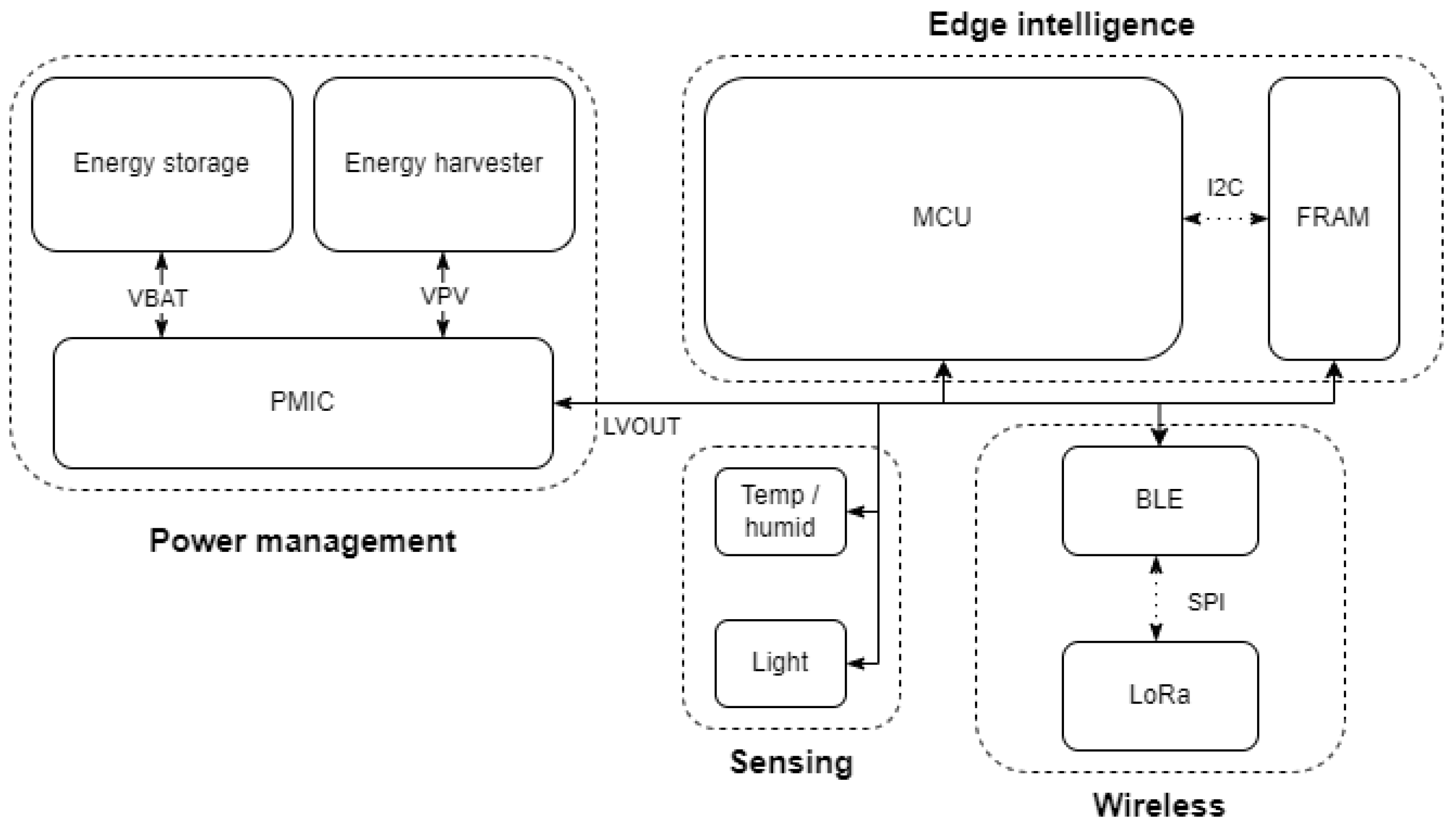
3. System Architecture

The HI-based module of this work is a low-power, energy autonomous device, targeted to Smart Agriculture applications. It integrates an SES for processing at the edge, environmental data acquisition, and data transfer, as well as a diffraction grating to enable the creation of a spectrometer. The module can be paired with a smartphone on demand by the user, to additionally allow the capture of high-resolution hyperspectral images. This section details the specifications and architecture of the SES of this work. The characteristics of the diffraction grating, when functioning as a spectral filter, are also given. Finally, the manufacturing and assembly of the HI-based module are presented.

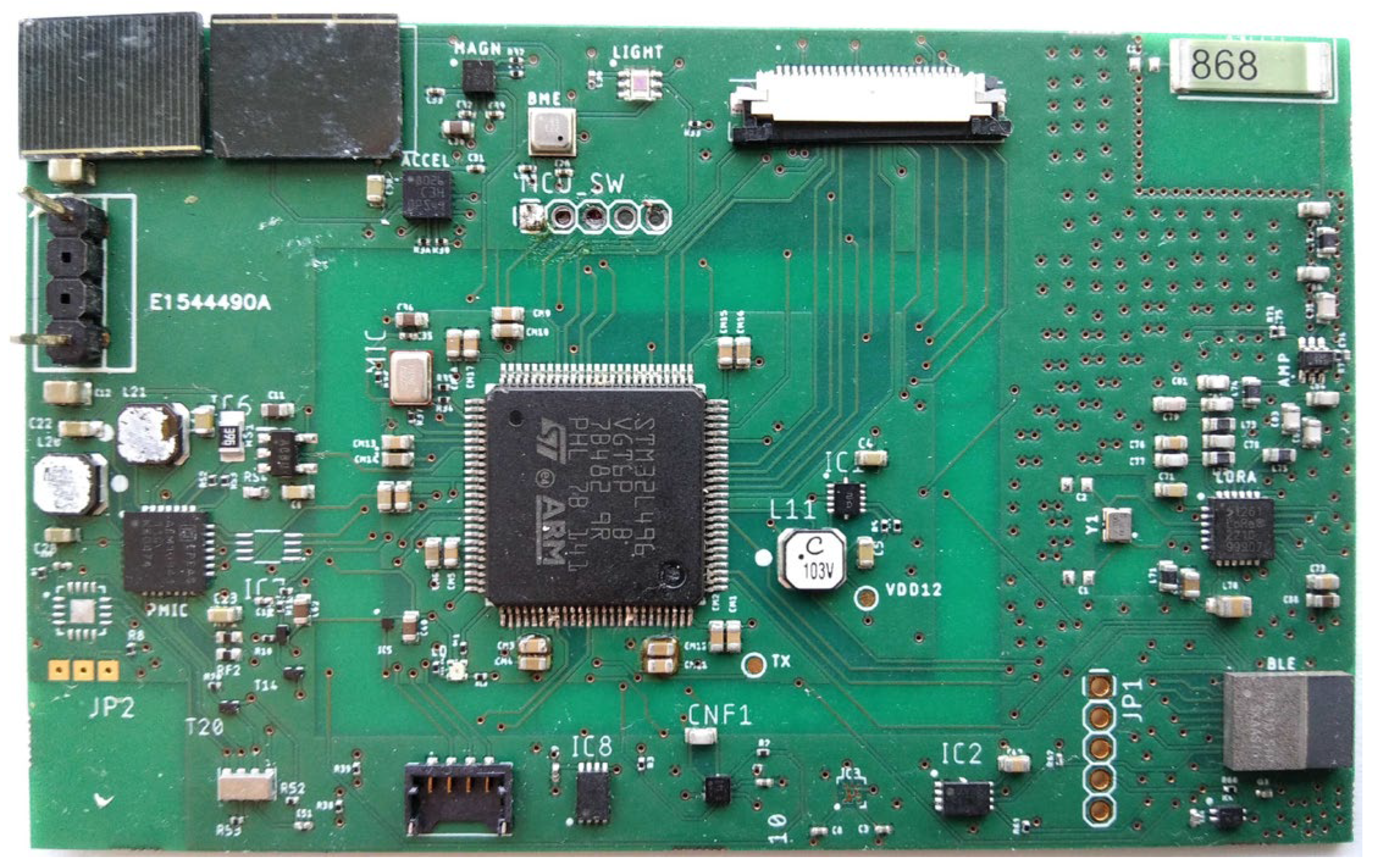
3.1. Hardware and Internet of Things Sensors

The proposed SES of this paper is used for autonomous data acquisition and processing on the edge. It was specifically designed and developed with an emphasis on low-power consumption and miniaturized dimensions. An initial version of the system was first presented by Kouzinopoulos et al. (2019) [50], with the introduction of an autonomous embedded system with miniaturized dimensions that harvested energy from PV cells to power sensors and communication ICs. However, an ARM Cortex-M0 MCU was utilized by Kouzinopoulos et al. that is not capable enough for the models of this work. Moreover, a different set of sensors was used. The system, with the addition of a Cortex-M4 MCU, the BME680 gas sensor, and the CCS811 air quality sensor, as well as the HM01B0 ultra-low-power CMOS image sensor, was evaluated by Papaioannou et al. (2023) [51] for low-power fire detection and crowd counting. It harvested energy from indoor illumination, using optimized variants of the MLP and YOLOv5 algorithms. Similar systems are very prevalent in the literature for Smart Agriculture applications, incorporating data acquisition from on-board sensors and processing at the edge, such as La Rosa et al. (2022) [52]. The groundwork for the power management architecture of the SES used in this paper was explored by Meli et al. (2023) [53], where the design of an energy autonomous low-power BLE node was described, capable of working under an illuminance as low as 5 lux. This is the first time that this system is used for autonomous decision-making on the edge, in the context of Smart Agriculture.

3.1.1. System Specifications

The system has the dimensions of a credit card, approximately 89 × 51 mm, and a thickness of less than 3 mm. It consists of several components, specifically integrated with an emphasis on low-power consumption and miniaturization, as summarized in

Table 2. Components integrated for low-power consumption and miniaturization.

Part No	Functionality	Manufacturer
Processing
STM32U5A5ZJ	MCU	ST
MB85RC64TAPN-G-AMEWE1	FRAM	Fujitsu Semiconductor
Sensors
MS1089	Temperature	Microdul
BME680	Environmental	Bosch
Power
EXL1-1V20	PV harvester	Lightricity
AEM10941	PMIC	E-Peas
GEB201212C	Battery	PowerStream
Communication
RSL10	Bluetooth Low Energy	Onsemi
SX1261	LoRa	Semtech

below.

More specifically, for edge processing, the STM32U5A5ZJ MCU from ST was used, based on the Cortex-M33 RISC instruction set architecture of ARM that can operate at a variable frequency of up to 160 MHz. The processor includes 4 Mbyte of flash memory and approximately 2.5 Mbyte of SRAM and features a single-precision floating point unit. Moreover, it features a 32 Kbyte instruction cache and 16 Kbyte data cache. The MCU can operate in seven different low-power modes, to achieve the best balance between power consumption, start-up time, as well as the number of available peripherals and wake-up sources. The modes include Run mode; Sleep mode; Stop 0–3, and Standby, as well as a Shutdown mode. During Run mode, it has 18.5 μA/MHz energy consumption.

For energy harvesting from solar light, the EXL1-1V20 PV cells (from Lightricity Ltd., Oxford, UK) were used. Each cell has more than 20 μW/cm² power density and more than a 30–35% efficiency under a white LED and fluorescent spectrum. The cells can produce up to approximately 0.1 mA of current for 1 V of voltage, under 1000 lux of illuminance. The system includes two EXL1-1V20-SM cells, each with a surface of 1 cm², yielding a total active surface of 2 cm². The cells were connected in parallel, in order to increase the output current of the energy harvester, as depicted in the upper left part of Figure 1.

To regulate, convert, control, and optimize the energy flow between the PV cells and the battery, as well as between the battery and the different components of the system, the AEM 10941 Power Management Integrated Circuit (PMIC) from E-peas was used. To store the excessive energy produced by the PV harvester, the Powerstream GEB201212C battery with a capacity of 10 mAh was used.

To store the data acquired by the system’s environmental sensors, as well as interim data from the ML algorithms developed for this paper, the MB85RC64TAPN-G-AMEWE1 64 KB low-power, non-volatile FRAM memory was used. The memory can be switched off between transfers in order to conserve energy and be put into sleep mode, which reduces quiescent current consumption.

For temperature sensing, the MS1089 temperature sensor from Microdul was used. The sensor can operate at 1.8 V, with 4 nA quiescent current between measurements and approximately 68 nA current consumption at 1 measurement per minute. For environmental sensing, including air humidity and air pressure, as well as Volatile Organic Compounds (VOCs) measurement, the BME680 environmental sensor was utilized. The sensor has 0.15 μA quiescent current, 3.7 μA current consumption at 1 Hz for humidity and pressure sensing, and 0.1 mA for VOCs measurements in ultra-low-power mode. For light sensing, the TI OPT3001 sensor was used.

For short-range communication, the system utilizes Bluetooth Low Energy (BLE) with the use of RSL10, an ultra-low-power IC. The IC has 3 mA peak Rx current consumption at 3 V and 4.6 mA peak Tx current consumption at 0 dBm at 3 V. For long-range communication, the Semtech SX1261 LoRa transceiver is used, with 4.2 mA of active receive current.

All sensing components, as well as BLE, are connected to the MCU via the I2C interface. LoRa is connected to the MCU via the BLE IC using SPI. A high-level architecture of the proposed SES is depicted in Figure 2.

3.2. Diffraction Grating

The diffraction grating enables the creation of spectrometers like the proposed HI-based module, which attaches to a smartphone camera for capturing spectral images. The specific diffraction grating used is the Edmund Optics (https://www.edmundoptics.eu/, accessed on 26 March 2024) transmission diffraction grating #49-580 (600 Grooves, 25 mm Sq, 28.7° Groove Angle Grating, Edmund Optics, Barrington, NJ, USA). Positioned in front of the smartphone’s camera sensor, this diffraction grating, with dimensions of 25 × 25 × 3 mm, allows data capture across the visible spectrum (400–700 nm). For the present study, the decision to use the wavelength range (400–700 nm) was based on a previous study by Stuart et al. [54]. Positioning the diffraction grating in front of the camera transforms the device into a spectral imaging system [54].

The use of diffraction gratings provides versatility, as they can be employed with different wavelength ranges depending on the application. This adaptation of diffraction gratings on the camera sensor provides the capability to separate the spectrum into individual wavelengths. Consequently, light can be effectively dissected into its spectral components based on their distinct wavelengths [55,56]. Unlike smartphone cameras, which are not specifically tailored for spectral analysis applications, placing the diffraction grating in front of a smartphone’s camera sensor allows the smartphone to capture the diffraction spectrum as an image.

3.3. Additive Manufacturing

The HI-based module was designed with a focus on portability and lightweight characteristics, making it easily adaptable to a mobile phone’s camera. Great attention was given to all dimensions of the HI-based system. The dimensions and properties of the diffraction grating and SES were carefully examined, and their respective recesses were designed to ensure proper functionality. The design process was carried out using SOLID-WORKS^® CAD Software (2022 SP2.0 Professional version) and the prototype was manufactured using the fused filament fabrication (FFF) technique.

The FFF 3D printer used for the manufacturing process was the Original Prusa i3 MK3S+. Prior to 3D printing, the printing parameters were configured using the Prusa Slicer 2.5.0 software. FFF was chosen as the fabrication method due to its speed, cost-effectiveness, and the wide variety of available materials [57,58]. However, other 3D printing techniques can also be employed, including selective laser sintering, selective laser melting, stereolithography, and more.

The material chosen for the HI-based module prototype was PETG (polyethylene terephthalate glycol), supplied in filament form with a 1.75 mm diameter. PETG is known for its ability to withstand and remain durable in hot weather conditions and it is also a recyclable material [19,59].

The 3D printing parameters for PETG were as follows: the printing temperature (nozzle temperature) was set to 245 °C and the 3D printer bed temperature was set at 80 °C. The nozzle diameter employed was 0.4 mm, the layer height was set to 0.2 mm, and a fill density of 20% was chosen to strike a balance between lightweight design and fulfilling usage requirements.

Figure 3 illustrates all the components that make up the HI-based module, comprising three 3D-printed parts and one commercial screw. These components, including the “Primary component” (1), “Secondary component” (2), “Screw” (3), and “Screw cap” (4), are assembled to enable the HI-based module’s attachment to a mobile phone’s (7) camera. The length of the HI-based module was designed to be 90 mm [54], determined to be an appropriate distance from the entry point of the light at the edge of the HI-based module, ensuring satisfactory capture of the diffraction spectrum. Finally, the “Primary component” features specially designed slots for the “Diffraction Grating” (5) and the “SES” (6).

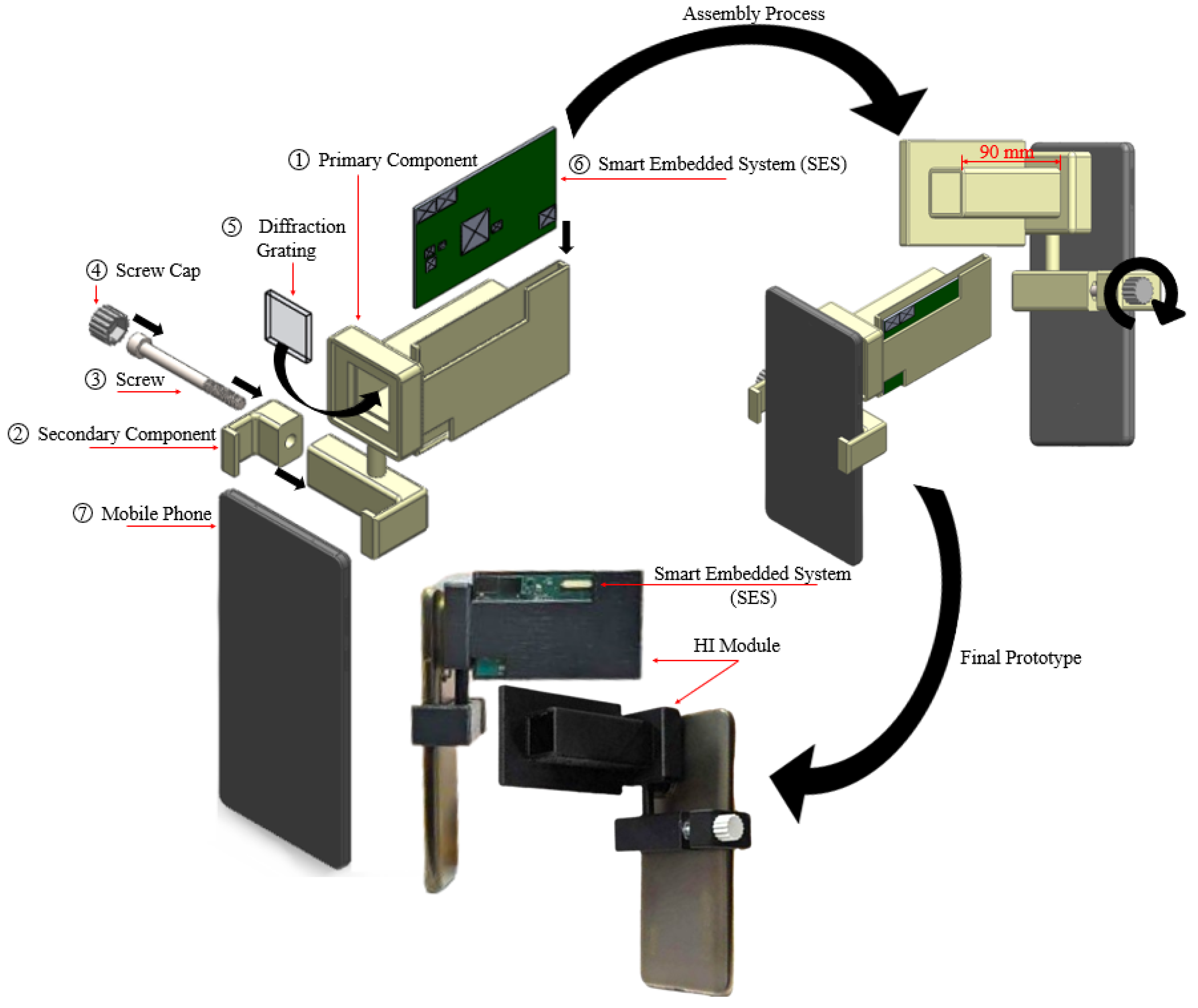
3.4. Assembly Process

In regard to the assembly and integration of all the components required for constructing the HI-based system and connecting it to a mobile phone, Figure 3 provides a comprehensive visual representation of this entire process. It provides isometric views of the HI-based system, showcasing the assembled CAD files and the final prototype. Specifically, within the figure, the screw cap (4) is seen positioned atop the screw (3), facilitating convenient user manipulation for rotation. The screw then interfaces with the secondary component (2) of the HI-based module, before engaging with the primary component (1).

Moreover, Figure 3 offers insights into the attachment of the diffraction grating (5) to the HI-based module. The diffraction grating seamlessly fits into the specially designed recess within the module. To ensure stability throughout the HI-based system’s operation, the diffraction grating is firmly affixed using silicone. Furthermore, the SES is securely placed within a purpose-built slot. The SES resides within a specifically shaped slot, designed to accommodate easy insertion and removal, with particular regions of the card exposed to collect precise environmental data. These thoughtful design considerations prioritize user-friendly assembly and disassembly, while maintaining stability during use.

Lastly, Figure 3 provides guidance on attaching the HI-based system to a mobile phone’s camera. The HI-based module, which includes the SES, can be affixed to devices of different dimensions. This versatility is achieved by allowing users to adjust its size through the rotation of the screw cap, facilitating the use of the HI-based system on various devices.

4. Deep Learning Integration

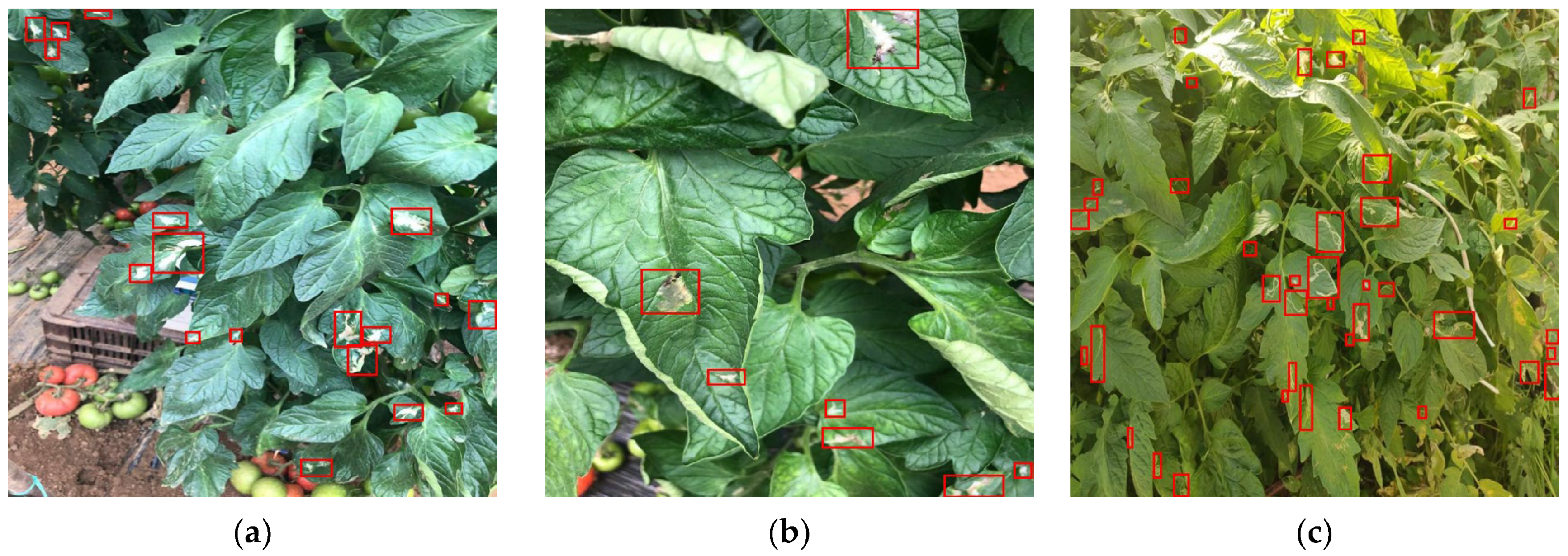
This section outlines the dataset utilized, details the lightweight object detection models implemented, and describes their integration on the proposed SES to detect T. absoluta infestation on-field, using the custom YOLOv5 algorithm.

4.1. Dataset

This study employs a dataset captured in RGB format under real-life conditions in fields and greenhouses, clearly depicting the damage caused by T. absoluta on tomato plants [49]. It comprises 659 images, split into 396 for training and 263 for validation, each annotated with bounding boxes around the areas of damage, executed by expert agronomists. These images and annotations were obtained from the EDEN Library (https://edenlibrary.ai, accessed on 26 March 2024). There are a total of 5443 annotations for the training set and 3267 for the validation set, making up 8710 annotations altogether. Figure 4 provides a visual representation, showcasing sample images that depict the characteristic damage caused by T. absoluta on tomato leaves.

The selection of the RGB dataset was based on the spectral capabilities of the diffraction grating used in this study, as specified in Section 3.2. Given that this particular diffraction grating facilitates data capture across the visible spectrum, RGB images were suitable for demonstration purposes. However, in addition to simple demonstration, the dataset also serves as a fundamental resource for pre-training models, with the potential for subsequent fine-tuning using a custom dataset tailored to alternative diffraction gratings placed into the 3D-printed module. A modification to the diffraction grating with a new one capable of capturing data beyond the visible spectrum holds considerable promise for HI, enabling comprehensive analyses of diverse agricultural practices, including diseases, pests, fungi, and overall crop health [12,15]. Furthermore, due to the lack of readily available datasets that meet our specific needs, this approach emerges as the most feasible.

4.2. Methodology

The proposed methodology focuses on sparse training, pruning, and fine-tuning to create lightweight DL models optimized for efficiency. Optimization of the model was pursued through sparsity training based on the Batch Normalization (BN) layer coefficient gamma pruning [61].

4.2.1. Sparse Training

BN [62] facilitates rapid convergence and enhances generalization performance. A BN layer normalizes internal activations using statistics from the mini batch. For an input $z_{in}$ and output $z_{out}$, of a BN layer, and given the current mini batch $B$, the BN layer executes the transformation:

$$\widehat{z}=\frac{z_{in}-{\mu }_B}{\sqrt{{\sigma }_B^2}+\epsilon };z_{out}=\gamma \cdot \widehat{z}+\beta$$

(1)

where ${\mu }_B$ is the batch mean and ${\sigma }_B^2$ is the batch variance of the input activations over batch $B$. The parameters $\gamma$ and $\beta$ are trainable and perform affine transformations (scaling and shifting), allowing the linear transformation of normalized activations to various scales.

For pruning purposes, the coefficient $\gamma$ in the BN layer is crucial. A small $\gamma$ leads to a proportionally low activation $z_{out}$, forming the basis for channel pruning within the BN layer. To achieve sparsity in $\gamma$, an L1 regularization constraint is added to the loss function [61]. The total loss $\mathcal{L}$ includes the original loss function $\mathcal{l}$ and the L1 regularization applied on $\gamma$ values:

$$\mathcal{L}={\sum }_{\left(x,y\right)}\mathcal{l}\left(f\left(x,w\right),y\right)+\lambda \cdot {\sum }_{\gamma \in \Gamma }g\left(\gamma \right),$$

(2)

where $x$ and $y$ are the input and output of the training, respectively; $w$ denotes the trainable weights in the network; the first sum term corresponds to the normal training loss; $g(\cdot )$ is a sparsity-induced penalty on the scaling factors; and $\lambda$ is the penalty factor that balances the two terms. Here, $g\left(s\right)=\left|s\right|$, which is known as L1-norm. The gradient descent algorithm optimizes the loss.

4.2.2. Pruning

After training, pruning is carried out [63]. Pruning reduces the model’s complexity and improves its efficiency to selectively remove less important neurons or connections. It is essential that the threshold does nοt surpass any channel BN’s maximum gamma. The pruning is then performed based on a defined cutting ratio, which determines the extent of reduction in the model’s size or complexity. Pruning a BN layer requires removing the previous layer’s convolution kernel and adjusting the following convolution layer’s corresponding channel. Pruning thresholds are critical in this process, serving as the criteria or limits that dictate which channels or neurons are considered less important and, thus, eligible for removal, ensuring a balanced trade-off between model simplicity and performance retention.

4.2.3. Fine-Tuning

Post-pruning, the model is fine-tuned. This step refines the pruned model, ensuring efficient performance without unnecessary parameters. Through this process, the model is optimized using a gradient descent algorithm. By fine-tuning the pruned model, it becomes more proficient at accurately capturing intricate patterns and features within the data, thereby enhancing its predictive capabilities.

4.3. Deep Learning Models

In this study, a custom version of the YOLOv5 [60] model was employed. The core architecture of the model, the CSP-Darknet53 backbone, was maintained, but with the following adjustments to its scale: a depth multiple of 0.33 and a width multiple of 0.10 was used. This resulted in a total of 326,562 parameters. Both the head and the neck of the original YOLOv5 model were retained without alteration. The custom YOLOv5 was fine-tuned for the detection of T. absoluta in tomato crops. Optimization of the model was pursued through sparsity training based on BN layer co-efficient gamma pruning, aiming to refine the model’s efficiency and effectiveness in recognizing and classifying the target in diverse crop environments.

No constraints were imposed on all BN layer gamma values. Specifically, layers with shortcuts, as found in the bottleneck structure of the C3 structure in YOLOv5, were left unpruned to retain the tensor dimension suitable for addition. Without the imposition of the L1 regularization constraint, the gamma distribution of the post-training BN layer resembles a normal distribution.

4.4. Model Training

The initial training was conducted using the AdamW [64] optimizer over 300 epochs with a 0.001 learning rate, decayed to 0.1. The momentum was set to 0.937. A warmup period was implemented during the first 3 epochs. The batch size was set to 32. All images were resized to 480 × 480 pixels for all experiments. Sparsity training was further applied for 100 epochs with the same hyper-parameters as base training and using the pre-trained weights of base training. Subsequently to sparsity training, pruning was applied at various thresholds, ranging from 10% to 30%. Finally, fine-tuning of the pruned models was executed across 100 epochs with the same hyper-parameters as base training.

The training process was carried out on a high-performance computing setup, equipped with an Intel^® Xeon^® processor running at 2.30 GHz, a Tesla T4 GPU with 16 GB of VRAM, and 12 GB of system RAM.

4.5. Evaluation Metrics

For the evaluation of the models, the COCO detection metrics [37] were utilized. This included the mean Average Precision (mAP) at an Intersection over Union (IoU) threshold of 0.5, denoted as mAP₅₀. It gives a single metric that reflects the model’s ability to correctly identify and locate objects. Additionally, precision and recall metrics were also reported. Precision measures the accuracy of the positive predictions, while recall assesses the model’s ability to detect all relevant instances. The evaluation further considered the model parameters, model size, and the computational intensity in terms of Giga-Floating Point Operations Per Second (GFLOPs).

4.6. Implementation in the Embedded System

The proposed version of YOLOv5 was developed on the PyTorch framework, in a similar manner to the original YOLOv5. Thus, conversion to TensorFlow Lite Micro (TFLM) was necessary before loading to the embedded platform [31]. The conversion process from PyTorch [65] to TFLM initiates with the conversion of the PyTorch model to Open Neural Network Exchange (ONNX) format. Subsequently. The onnx2tf library (https://pypi.org/project/onnx2tf/, accessed on 26 March 2024) was used to convert the ONNX file to TensorFlow format. Finally, the TensorFlow file was converted to TFLM format, ensuring compatibility with embedded platforms, followed by the transformation into C code, prepared for uploading onto the embedded platforms.

To optimize the performance of the model in terms of execution time and memory requirements, quantization techniques were applied. There are two different methods for neural network quantization, Post-Training Quantization (PTQ) and Quantization-Aware Training (QAT). The primary distinction between PTQ and QAT lies in the stage at which the scale is computed. PTQ involves computing the quantized model after the network has completed training, typically confined to FP16 or INT8 quantization. In contrast, QAT calculates the quantized model during the training phase. PTQ with binary 32 and 16 and integer 8 were applied in this article.

5. Results and Discussion

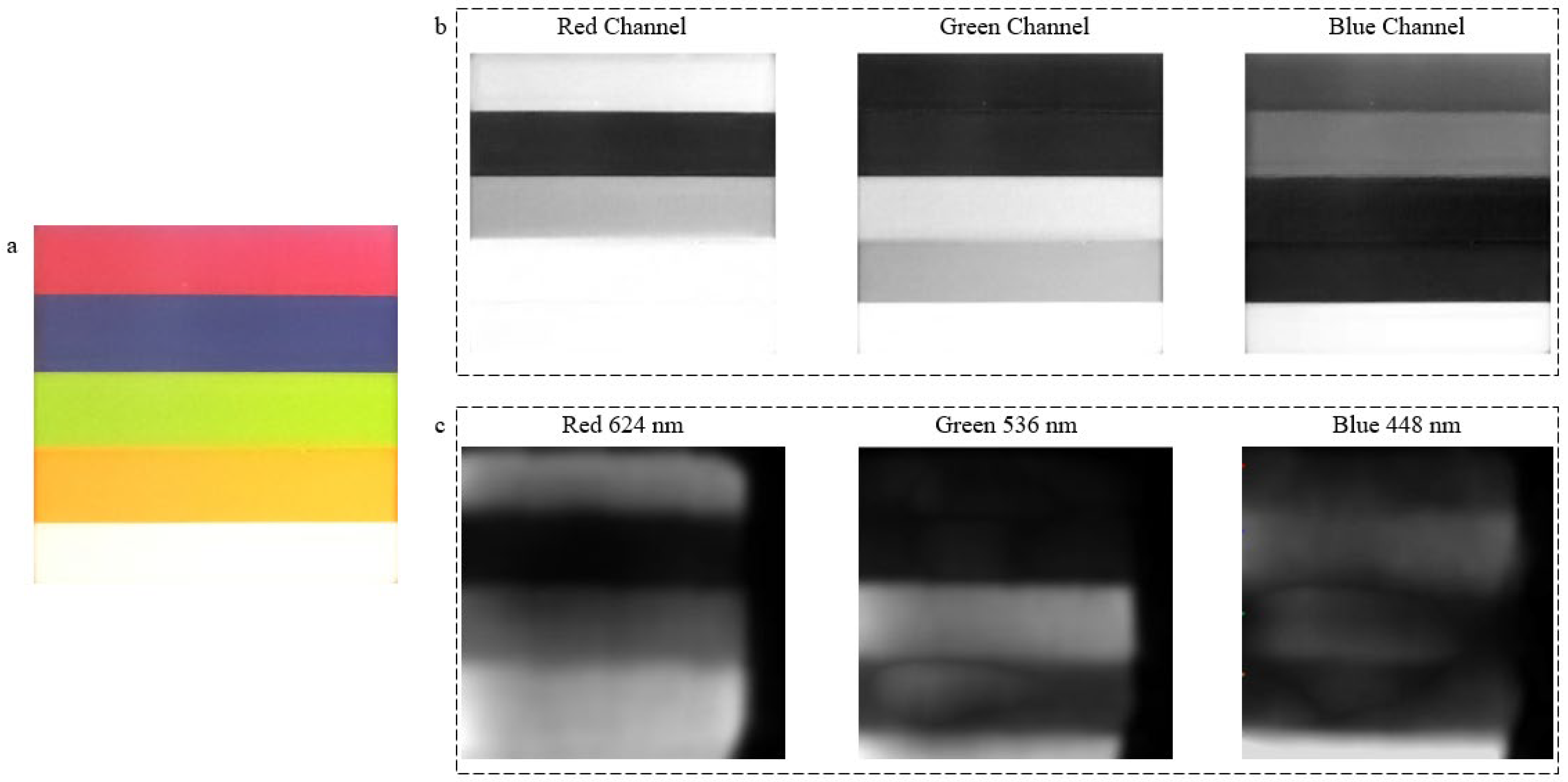
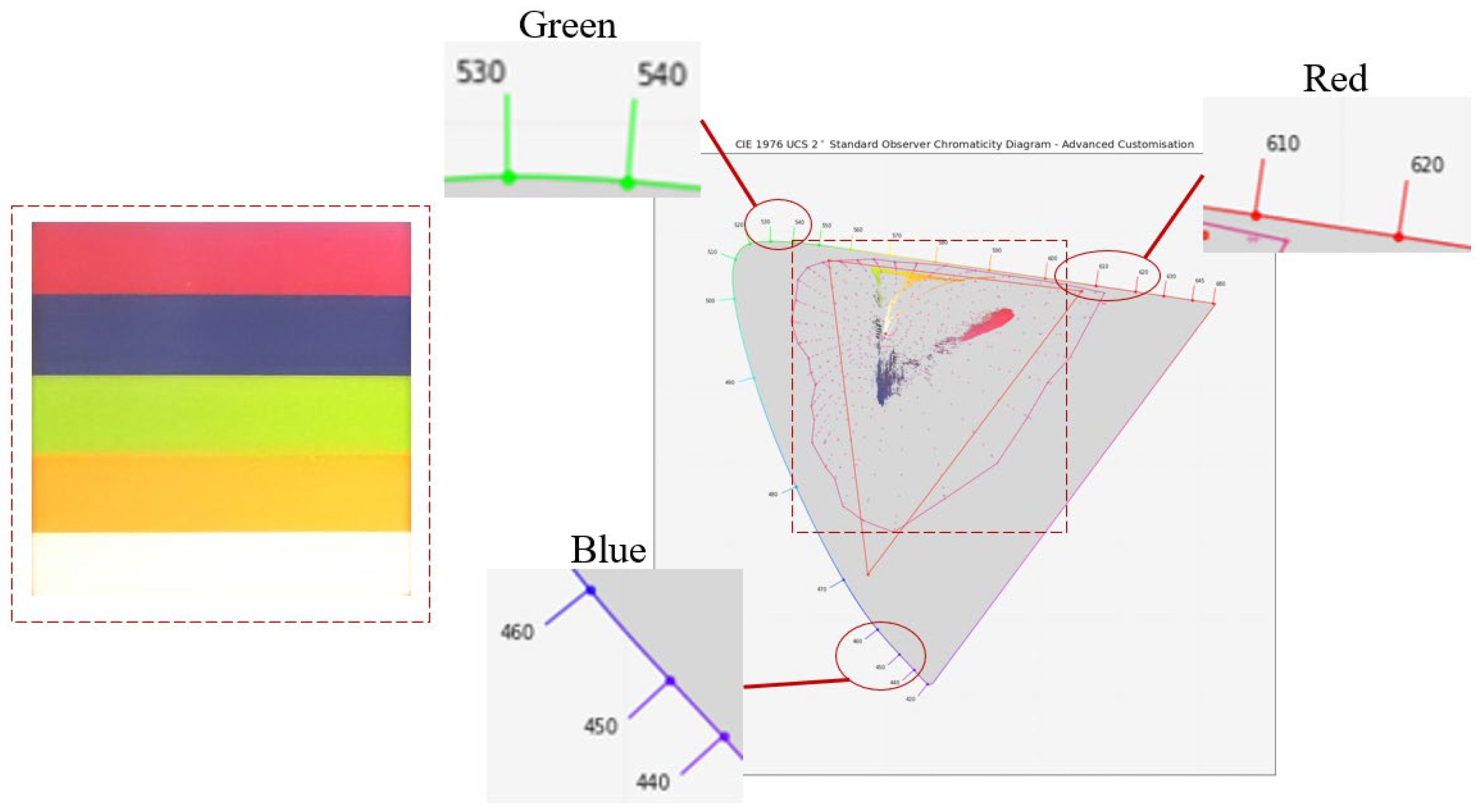
5.1. Proof of Concept Using Spectral Images from a 3D-Printed Multi-Color Box

For the evaluation of the images captured using the HI-based module as a proof of concept, the same 3D-printed multi-color box was utilized, as used in a prior study where a hyperspectral camera was developed [19]. The multi-color box was captured using a smartphone’s camera equipped with the HI-based system, as depicted in Figure 3. Subsequently, individual spectral images for the red, green, and blue channel were extracted. The exported red channel image corresponds to a wavelength of 624 nm, the green channel to 536 nm, and the blue channel to 448 nm. Figure 5 presents a comparative analysis between the results of the HI-based system in and the spectral images from the hyperspectral camera in a prior study, as shown in Figure 5c, revealing distinct and accurate color representations. Specifically, Figure 5b highlights the vivid and correct display of red, green, and blue colors, each appearing brighter in its respective channel, while the white color is evident in all images, due to its broad spectral nature.

Compared to a similar hyperspectral device developed by Stuart et al. [54], the pro-posed HI-based module is designed with a focus on functioning in external environments, primarily for agricultural applications. In outdoor settings, controlled laboratory conditions are not possible, resulting in the proposed HI-based system’s captured images exhibiting a spectral overlap phenomenon (https://flowcore.syr.edu/help/spectral-overlap/, accessed on 26 March 2024) [66]. However, the proof of concept presented in Figure 5 demonstrates that even with images containing overlapped spectra information, the colors are detected at the correct wavelengths.

In order to understand the colors captured within the 3D-printed multi-color box and its color space, the data of the images were visualized in a CIE 1976 UCS chromaticity diagram (https://colour.readthedocs.io/en/latest/index.html, accessed on 26 March 2024). The extracted diagram was constructed based on the decoded RGB data of the image and provides a comprehensive visualization of the wavelengths associated with each color that exists within the multi-color box. In Figure 6, the image of the 3D-printed multi-color box reveals that the red, green, and blue colors are near the wavelengths of 624 nm, 536 nm, and 448 nm, respectively. This detailed representation provides important information about the exact colors the HI-based module captures, helping to better understand its ability to image different wavelengths.

5.2. Proof of Concept Using Spectral Images from Agricultural Leaves

To extend the assessment of the HI-based system’s capabilities, another proof of concept was executed using a leaf. This attempt aimed to garner insights for potential agricultural applications in the future. Using the leaf image, individual spectral images were generated for the red, green, and blue channels. Figure 7 portrays the original spectral image captured by the HI-based module, alongside the three additional exported images. As anticipated, the green channel at 536 nm reveals the lightest hue, aligning with the predominantly green color of the leaf, underscoring the camera’s precise color capture capability. In contrast, the blue channel at 448 nm exhibits the darkest shade.

5.3. Deep Learning Models’ Results

Adjusting the resolution of the images for processing in object detection frequently leads to a diminished mAP, as the essential details crucial for precise object recognition and localization tend to get lost. Nonetheless, object detection involves the complex task of both identifying objects and accurately regressing their locations within the image, which naturally complicates the achievement of elevated mAP figures. The custom YOLOv5 model, incorporating a depth multiple of 0.33 and a width multiple of 0.10, was validated in the initial T. absoluta dataset to assess its performance. The base model has a size of 926 KB, featuring 326,562 parameters at 1.0 GFLOPs. The base model without the incorporation of sparsity achieved an mAP₅₀ of 0.46, demonstrating a precision of 0.54 and a recall of 0.46. This base model was used as a pre-training checkpoint for sparsity training. Following the base training, models with varying levels of sparsity were trained, as shown in

Table 3. Initial experiment results with custom YOLOv5 (depth 0.33, width 0.10).

Sparsity	mAP50	Precision	Recall	Prune Threshold
0	0.460	0.546	0.467	-
0.00001	0.462	0.605	0.437	0.65710
0.00005 1	0.465	0.548	0.476	0.7344
0.0001	0.460	0.570	0.462	0.6234
0.0005	0.455	0.551	0.466	0.3746
0.001	0.453	0.536	0.467	0.2905
0.005	0.44	0.544	0.451	0.1471
0.01	0.433	0.563	0.425	0.0754

¹ Bold row indicates the best performing model in terms of mAP₅₀.

. The introduction of minimal sparsity (0.00001) slightly enhanced the mAP₅₀, significantly increasing precision while slightly reducing recall. As sparsity levels increased, mAP₅₀ showed minor fluctuations, with a peak performance of 0.465 observed at a sparsity level of 0.00005 with a precision of 54.8%.

Subsequently, models were pruned at a maximum rate of 30% to reduce their size, aiming for a balanced trade-off between mAP₅₀ and parameters. Models showing significant loss in detection capability post-pruning were discarded (

Table A1. Pruning of sparsed trained custom YOLOv5 (depth 0.33, width 0.10).

Sparsity	Pruning Ration	Params	GFLOPs	mAP50	Size
0.00001	10%	286,535	0.9	0.0134	753 KB
0.00001	20%	245,420	0.8	0.0032	673 KB
0.00001	30%	208,185	0.7	0.0023	600 KB
0.00005	10%	286,249	0.9	0.0451	753 KB
0.00005	20%	244,197	0.8	0.0042	670 KB
0.00005	30%	202,607	0.7	0.0026	588 KB
0.0001	10%	285,034	0.9	0.1708	751 KB
0.0001	20%	239,037	0.8	0.0061	660 KB
0.0001	30%	201,337	0.7	0.0053	586 KB
0.0005	10%	279,444	0.9	0.4483	740 KB
0.0005	20%	237,086	0.8	0.4482	657 KB
0.0005	30%	195,702	0.7	0.3757	575 KB
0.001	10%	282,376	0.9	0.4390	745 KB
0.001	20%	237,293	0.8	0.4533	657 KB
0.005	10%	288,219	0.9	0.4146	757 KB

Bold rows indicate selected models for fine-tuning.

). The remaining models, demonstrating more promising mAP₅₀ values, were selected for fine-tuning.

Table 4. Fine-tuned pruned models’ results with custom YOLOv5 (depth 0.33, width 0.10).

Sparsity	Prune Ratio	Params.	GFLOPs	Size	mAP50	Precision	Recall
0.0001	10%	285,034	0.9	751 KB	0.433	0.499	0.456
0.0005	10%	279,444	0.9	740 KB	0.442	0.499	0.474
0.0005	20%	237,086	0.8	657 KB	0.437	0.524	0.452
0.0005 3	30%	195,702	0.7	575 KB	0.434	0.497	0.467
0.001 2	10%	282,376	0.9	745 KB	0.445	0.558	0.434
0.001	20%	237,293	0.8	657 KB	0.439	0.529	0.446
0.005	10%	288,219	0.9	757 KB	0.424	0.51	0.45

² Bold row indicates the best performing model. ³ Underlined row indicates the model with the lowest size.

shows the results of the fine-tuned pruned models with the custom YOLOv5. Models with 0.0001 and 0.0005 sparsity levels pruned at 10% with similar sizes around 750 KB, with GFLOPs at 0.9, achieved mAP₅₀ values of 0.43 and 0.44, respectively. Increasing the pruning ratio to 20% and 30% in the 0.0005 sparsity model led to further size reduction, with a marginal decrease in mAP₅₀. Meanwhile, models with 0.001 sparsity pruned at 10% and 20% offered a balance between size and detection accuracy, with mAP₅₀ values in the 0.43 to 0.44 range.

For the optimal trade-off between size and mAP₅₀, the model with a sparsity rate of 0.0005, pruned at 30%, emerged as the optimal choice. It demonstrated a slight reduction in mean mAP₅₀, dropping from 0.465 to 0.434, which constitutes a decrease of approximately 6.67%. More significantly, the model size was reduced from 926 KB to 575 KB, amounting to a decrease of 37.90%. This streamlined model was subsequently implemented in the embedded system.

5.4. Deep Learning Models’ Results on the Embedding System

To further evaluate the performance of the custom YOLOv5 model in detecting T. absoluta, the version implemented on the embedded system was validated using the T. absoluta dataset.

Table 5. Results of the custom YOLOv5 for different quantization precisions (sparsity 0.0005, pruning 30%).

Quantization Precision	mAP50	Precision	Recall	Size	RAM Usage	Execution Time
32-bit	0.434	0.497	0.467	1.165 KB	2.423 KB	17.22 min
16-bit	0.415	0.476	0.442	655 KB	1.945 KB	8.55 min
8-bit	0.398	0.459	0.425	403 KB	1.393 KB	4.15 min

illustrates the results of deploying the custom YOLOv5 model across different quantization precisions, maintaining a constant sparsity of 0.0005 and a pruning rate of 30%. The frequency of the evaluation platform, as detailed in Section 3.1.1, was 160 MHz. The impact of different quantization precisions on all metrics (mAP₅₀, precision, size, ram usage, and execution time) is noticeable. Specifically, for 32-bit precision, the model achieved an mAP₅₀ of 0.434, precision of 0.497, and an execution time of 17.22 min, accompanied by a model size of 1.165 KB and a RAM usage of 2.423 KB. There was a noticeable reduction in these metrics as the precision decreases. The 16-bit precision exhibits an mAP₅₀ of 0.415, precision of 0.476, and an execution time of 8.55 min, with a smaller model size of 655 KB and a RAM usage of 1.945 KB. In percentage terms, this represents a reduction of 4.47% in mAP50, 56.04% in memory size, 22.25% in RAM usage, and 67.29% in execution time, compared to the 32-bit precision. Similarly, the 8-bit precision exhibits a reduction in mAP₅₀ by 8.65%, in memory size by 198.85%, in RAM usage by 53.98%, and in execution time by 122.32%, compared to the 32-bit precision.

The results from deploying the custom YOLOv5 model on the embedded system may not be directly comparable to the methods executed on more powerful hardware setups. The observed reduction in mAP₅₀, followed by a reduction in memory size, RAM usage, and execution time reflect the compromises made to accommodate the constraints of the embedded system. Under the resource constraints of the low-power environment, these reductions are required to ensure that the customized YOLOv5 model remains functional.

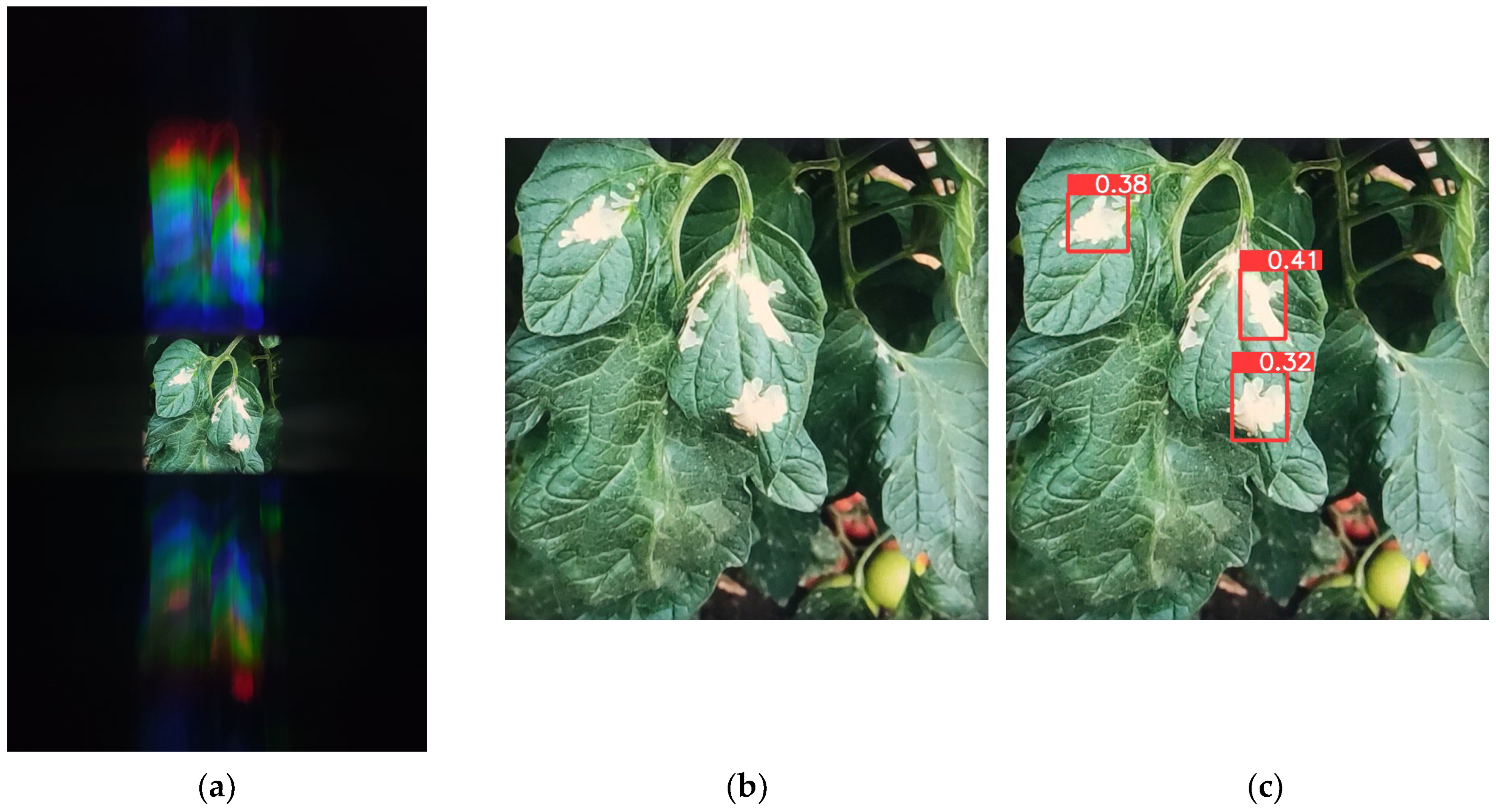
5.5. Proof of Concept in Detection of T. absoluta

To confirm the T. absoluta detection performance of the HI-based smart embedded system, the visible range capabilities of the diffraction grating used (400–700 nm) were leveraged. This choice offers advantages over conventional smartphone cameras, enhancing the capture of the red (R), green (G), and blue (B) channels for improved analysis. As depicted in Figure 8a,b, the original image, captured in RGB format in a greenhouse by the HI-based system attached to the smartphone camera, is cropped to retain only relevant details for the model. Subsequently, this cropped image serves as an input for the custom YOLOv5 8-bit model, generating the final result with distinct bounding boxes outlining areas affected by T. absoluta damage. This successful proof of concept not only underscores the immediate effectiveness of identifying and highlighting T. absoluta-inflicted damage on tomato leaves, but also positions the HI-based system for future applications.

In addition to capturing the image, a temperature of 27 °C, a humidity of 70%, and an illuminance of approximately 2000 lux was captured using the environmental and light sensors of the module. Temperature significantly affects the development, reproduction, and longevity of T. absoluta [67]. High humidity levels are also generally favorable for the reproduction and survival of the pest, as it tends to thrive in warm and humid conditions. Finally, light intensity can indirectly affect the pest’s behavior and activity. Through the analysis of the sensor data through a DSS capable of utilizing real-time data [21], farmers can gain a comprehensive understanding of the environmental conditions conducive to T. absoluta’s growth, development, survival, and reproduction.

6. Conclusions

This study introduces a lightweight, portable, and user-friendly HI-based smart embedded system for citizen science. Designed for seamless integration with smartphones equipped with cameras, this innovative citizen science tool offers energy autonomy, empowering farmers, communities, and citizens to effortlessly capture and relay crucial data on crop conditions, plant diseases, pest incursions, and crop monitoring. The HI-based module, based on a low-power ARM RISC architecture for energy efficiency, employs an optimized DL algorithm to showcase as a proof of concept the detection and identification of damage caused by the T. absoluta pest. This demonstration illustrates the potential applicability of similar DL algorithms for detecting various insects and fungal diseases.

The custom YOLOv5 method shows promising outcomes in identifying T. absoluta-inflicted damage on tomato leaves. Specifically, the model version implemented on the embedded system resulted in an mAP₅₀ of 0.398, a precision of approximately 50%, a compact model size of 403 KB, and RAM usage of 1.393 KB, contributing to social inclusion in the inspection of quarantine pests and invasive alien spread. Also, besides capturing images, the module acquires data from different sensors for further understanding of the environmental conditions that can affect the growth and reproduction of the detected insect or plant disease. By integrating this data, predictive models can be refined to anticipate and mitigate the impact of plant diseases and pest infections on crop yields, ensuring more resilient agricultural practices. Additionally, these integrated data have the potential to be connected to a DSS, offering valuable insights for informed decision-making in agricultural management.

As for the current installed diffraction grating used in the range of 400–700 nm, future studies can explore the replacement with various diffraction gratings featuring different wavelength ranges, extending into the Near Infrared Range (NIR) (over 700 nm). While the RGB dataset served its purpose for demonstration and initial model training, it is important to acknowledge that a hyperspectral dataset and a diffraction grating capable of capturing data beyond the visible spectrum can offer a more comprehensive understanding of agricultural phenomena. By utilizing the proposed DL pipeline, it is possible to adjust and fine-tune the models to accommodate new wavelength ranges, such as NIR, thereby enhancing the capability of hyperspectral imaging to detect and analyze a broader spectrum of spectral data. This potential hold promises to address specific agricultural application needs and opens doors to adapting the proposed HI-based smart embedded system to diverse agricultural concerns, including the detection of widespread fungal diseases.

In summary, the introduction of a novel HI-based module for citizen science represents a significant advancement in agricultural technology. By providing a user-friendly and accessible tool for surveillance, monitoring, and detection, this innovation opens doors for farm citizens, farmers, land managers, and the general public to actively engage in data collection and analysis. With its versatile applications, this tool holds the potential to revolutionize the way agricultural information is gathered and utilized, empowering individuals at every level of the agricultural landscape to contribute to improved practices and outcomes.

References

1. Dehnen-Schmutz, K.; Foster, G.L.; Owen, L.; Persello, S. Exploring the role of smartphone technology for citizen science in agriculture. Agron. Sustain. Dev. 2016, 36, 25. [Google Scholar] [CrossRef]
2. Brown, N.; Pérez-Sierra, A.; Crow, P.; Parnell, S. The role of passive surveillance and citizen science in plant health. CABI Agric. Biosci. 2020, 1, 17. [Google Scholar] [CrossRef] [PubMed]
3. Carleton, R.D.; Owens, E.; Blaquière, H.; Bourassa, S.; Bowden, J.J.; Candau, J.-N.; DeMerchant, I.; Edwards, S.; Heustis, A.; James, P.M.A.; et al. Tracking insect outbreaks: A case study of community-assisted moth monitoring using sex pheromone traps. FACETS 2020, 5, 91–104. [Google Scholar] [CrossRef]
4. Malek, R.; Tattoni, C.; Ciolli, M.; Corradini, S.; Andreis, D.; Ibrahim, A.; Mazzoni, V.; Eriksson, A.; Anfora, G. Coupling Traditional Monitoring and Citizen Science to Disentangle the Invasion of Halyomorpha halys. ISPRS Int. J. Geo-Inf. 2018, 7, 171. [Google Scholar] [CrossRef]
5. Meentemeyer, R.K.; Dorning, M.A.; Vogler, J.B.; Schmidt, D.; Garbelotto, M. Citizen science helps predict risk of emerging infectious disease. Front. Ecol. Environ. 2015, 13, 189–194. [Google Scholar] [CrossRef] [PubMed]
6. Garbelotto, M.; Maddison, E.R.; Schmidt, D. SODmap and SODmap Mobile: Two Tools to Monitor the Spread of Sudden Oak Death. For. Phytophthoras 2014, 4. [Google Scholar] [CrossRef]
7. de Groot, M.; Pocock, M.J.O.; Bonte, J.; Fernandez-Conradi, P.; Valdés-Correcher, E. Citizen Science and Monitoring Forest Pests: A Beneficial Alliance? Curr. For. Rep. 2023, 9, 15–32. [Google Scholar] [CrossRef] [PubMed]
8. Mkonyi, L.; Rubanga, D.; Richard, M.; Zekeya, N.; Sawahiko, S.; Maiseli, B.; Machuve, D. Early identification of Tuta absoluta in tomato plants using deep learning. Sci. Afr. 2020, 10, e00590. [Google Scholar] [CrossRef]
9. Wang, C.; Liu, B.; Liu, L.; Zhu, Y.; Hou, J.; Liu, P.; Li, X. A review of deep learning used in the hyperspectral image analysis for agriculture. Artif. Intell. Rev. 2021, 54, 5205–5253. [Google Scholar] [CrossRef]
10. Khan, A.; Vibhute, A.D.; Mali, S.; Patil, C.H. A systematic review on hyperspectral imaging technology with a machine and deep learning methodology for agricultural applications. Ecol. Inform. 2022, 69, 101678. [Google Scholar] [CrossRef]
11. Lu, B.; Dao, P.D.; Liu, J.; He, Y.; Shang, J. Recent Advances of Hyperspectral Imaging Technology and Applications in Agriculture. Remote Sens. 2020, 12, 2659. [Google Scholar] [CrossRef]
12. Avola, G.; Matese, A.; Riggi, E. An Overview of the Special Issue on ‘Precision Agriculture Using Hyperspectral Images’. Remote Sens. 2023, 15, 1917. [Google Scholar] [CrossRef]
13. Barbedo, J.G.A. A review on the combination of deep learning techniques with proximal hyperspectral images in agriculture. Comput. Electron. Agric. 2023, 210, 107920. [Google Scholar] [CrossRef]
14. Wang, Y.M.; Ostendorf, B.; Gautam, D.; Habili, N.; Pagay, V. Plant Viral Disease Detection: From Molecular Diagnosis to Optical Sensing Technology—A Multidisciplinary Review. Remote Sens. 2022, 14, 1542. [Google Scholar] [CrossRef]
15. Rayhana, R.; Ma, Z.; Liu, Z.; Xiao, G.; Ruan, Y.; Sangha, J. A Review on Plant Disease Detection Using Hyperspectral Imaging. IEEE Trans. AgriFood Electron. 2023, 1, 108–134. [Google Scholar] [CrossRef]
16. Teke, M.; Deveci, H.S.; Haliloğlu, O.; Gürbüz, S.Z.; Sakarya, U. A short survey of hyperspectral remote sensing applications in agriculture. In Proceedings of the 2013 6th International Conference on Recent Advances in Space Technologies (RAST), Istanbul, Turkey, 12–14 June 2013; pp. 171–176. [Google Scholar] [CrossRef]
17. Adão, T.; Hruška, J.; Pádua, L.; Bessa, J.; Peres, E.; Morais, R.; Sousa, J.J. Hyperspectral Imaging: A Review on UAV-Based Sensors, Data Processing and Applications for Agriculture and Forestry. Remote Sens. 2017, 9, 1110. [Google Scholar] [CrossRef]
18. Eli-Chukwu, N.C. Applications of Artificial Intelligence in Agriculture: A Review. Eng. Technol. Appl. Sci. Res. 2019, 9, 4377–4383. [Google Scholar] [CrossRef]
19. Pechlivani, E.M.; Papadimitriou, A.; Pemas, S.; Giakoumoglou, N.; Tzovaras, D. Low-Cost Hyperspectral Imaging Device for Portable Remote Sensing. Instruments 2023, 7, 32. [Google Scholar] [CrossRef]
20. Ahmad, F.F.; Ghenai, C.; Bettayeb, M. Maximum power point tracking and photovoltaic energy harvesting for Internet of Things: A comprehensive review. Sustain. Energy Technol. Assess. 2021, 47, 101430. [Google Scholar] [CrossRef]
21. Pechlivani, E.M.; Gkogkos, G.; Giakoumoglou, N.; Hadjigeorgiou, I.; Tzovaras, D. Towards Sustainable Farming: A Robust Decision Support System’s Architecture for Agriculture 4.0. In Proceedings of the 2023 24th International Conference on Digital Signal Processing (DSP), Rhodes, Greece, 11–13 June 2023; pp. 1–5. [Google Scholar] [CrossRef]
22. Miranda, M.M.M.; Picanço, M.; Zanuncio, J.C.; Guedes, R.N.C. Ecological Life Table of Tuta absoluta (Meyrick) (Lepidoptera: Gelechiidae). Biocontrol Sci. Technol. 1998, 8, 597–606. [Google Scholar] [CrossRef]
23. Urbaneja, A.; González-Cabrera, J.; Arnó, J.; Gabarra, R. Prospects for the biological control of Tuta absoluta in tomatoes of the Mediterranean basin. Pest Manag. Sci. 2012, 68, 1215–1222. [Google Scholar] [CrossRef]
24. Qazi, S.; Khawaja, B.A.; Farooq, Q.U. IoT-Equipped and AI-Enabled Next Generation Smart Agriculture: A Critical Review, Current Challenges and Future Trends. IEEE Access 2022, 10, 21219–21235. [Google Scholar] [CrossRef]
25. Brunelli, D.; Albanese, A.; d’Acunto, D.; Nardello, M. Energy Neutral Machine Learning Based IoT Device for Pest Detection in Precision Agriculture. IEEE Internet Things Mag. 2019, 2, 10–13. [Google Scholar] [CrossRef]
26. Gia, T.N.; Qingqing, L.; Queralta, J.P.; Zou, Z.; Tenhunen, H.; Westerlund, T. Edge AI in Smart Farming IoT: CNNs at the Edge and Fog Computing with LoRa. In Proceedings of the 2019 IEEE AFRICON, Accra, Ghana, 25–27 September 2019; pp. 1–6. [Google Scholar] [CrossRef]
27. Shivling, D.V.; Sharma, S.K.; Ghanshyam, C.; Dogra, S.; Mokheria, P.; Kaur, R.; Arora, D. Low cost sensor based embedded system for plant protection and pest control. In Proceedings of the 2015 International Conference on Soft Computing Techniques and Implementations (ICSCTI), Faridabad, India, 8–10 October 2015; pp. 179–184. [Google Scholar] [CrossRef]
28. Materne, N.; Inoue, M. IoT Monitoring System for Early Detection of Agricultural Pests and Diseases. In Proceedings of the 2018 12th South East Asian Technical University Consortium (SEATUC), Yogyakarta, Indonesia, 12–13 March 2018; pp. 1–5. [Google Scholar] [CrossRef]
29. Yashodha, G.; Shalini, D. An integrated approach for predicting and broadcasting tea leaf disease at early stage using IoT with machine learning—A review. Mater. Today Proc. 2021, 37, 484–488. [Google Scholar] [CrossRef]
30. Terentev, A.; Dolzhenko, V.; Fedotov, A.; Eremenko, D. Current State of Hyperspectral Remote Sensing for Early Plant Disease Detection: A Review. Sensors 2022, 22, 757. [Google Scholar] [CrossRef]
31. Hussain, T.; Shah, B.S.; Ullah, I.U.; Shah, S.M.; Ali, F.; Park, S.H. Deep learning-based segmentation and classification of leaf images for detection of tomato plant disease. Front. Plant Sci. 2022, 13, 1031748. [Google Scholar] [CrossRef]
32. Giakoumoglou, N.; Pechlivani, E.M.; Sakelliou, A.; Klaridopoulos, C.; Frangakis, N.; Tzovaras, D. Deep learning-based multi-spectral identification of grey mould. Smart Agric. Technol. 2023, 4, 100174. [Google Scholar] [CrossRef]
33. Georgantopoulos, P.S.; Papadimitriou, D.; Constantinopoulos, C.; Manios, T.; Daliakopoulos, I.N.; Kosmopoulos, D. A Multispectral Dataset for the Detection of Tuta Absoluta and Leveillula Taurica in Tomato Plants. Smart Agric. Technol. 2023, 4, 100146. [Google Scholar] [CrossRef]
34. Fernández, C.I.; Leblon, B.; Wang, J.; Haddadi, A.; Wang, K. Detecting Infected Cucumber Plants with Close-Range Multispectral Imagery. Remote Sens. 2021, 13, 2948. [Google Scholar] [CrossRef]
35. Nagasubramanian, K.; Jones, S.; Singh, A.K.; Sarkar, S.; Singh, A.; Ganapathysubramanian, B. Plant disease identification using explainable 3D deep learning on hyperspectral images. Plant Methods 2019, 15, 98. [Google Scholar] [CrossRef]
36. Moghadam, P.; Ward, D.; Goan, E.; Jayawardena, S.; Sikka, P.; Hernandez, E. Plant Disease Detection Using Hyperspectral Imaging. In Proceedings of the 2017 International Conference on Digital Image Computing: Techniques and Applications (DICTA), Sydney, Australia, 29 November–1 December 2017; pp. 1–8. [Google Scholar] [CrossRef]
37. Nguyen, C.; Sagan, V.; Maimaitiyiming, M.; Maimaitijiang, M.; Bhadra, S.; Kwasniewski, M.T. Early Detection of Plant Viral Disease Using Hyperspectral Imaging and Deep Learning. Sensors 2021, 21, 742. [Google Scholar] [CrossRef] [PubMed]
38. Feng, L.; Wu, B.; He, Y.; Zhang, C. Hyperspectral Imaging Combined with Deep Transfer Learning for Rice Disease Detection. Front. Plant Sci. 2021, 12, 693521. [Google Scholar] [CrossRef] [PubMed]
39. Bannerjee, G.; Sarkar, U.; Das, S.; Ghosh, I. Artificial intelligence in agriculture: A literature survey. Int. J. Sci. Res. Comput. Sci. Appl. Manag. Stud. 2018, 7, 1–6. [Google Scholar]
40. Giakoumoglou, N.; Pechlivani, E.M.; Tzovaras, D. Generate-Paste-Blend-Detect: Synthetic dataset for object detection in the agriculture domain. Smart Agric. Technol. 2023, 5, 100258. [Google Scholar] [CrossRef]
41. Giakoumoglou, N.; Pechlivani, E.M.; Katsoulas, N.; Tzovaras, D. White Flies and Black Aphids Detection in Field Vegetable Crops using Deep Learning. In Proceedings of the 2022 IEEE 5th International Conference on Image Processing Applications and Systems (IPAS), Genova, Italy, 5–7 December 2022; pp. 1–6. [Google Scholar] [CrossRef]
42. Liu, J.; Wang, R.; Xie, C.; Yang, P.; Wang, F.; Sudirman, S.; Liu, W. PestNet: An End-to-End Deep Learning Approach for Large-Scale Multi-Class Pest Detection and Classification. IEEE Access 2019, 7, 45301–45312. [Google Scholar] [CrossRef]
43. Liu, J.; Wang, X. Tomato Diseases and Pests Detection Based on Improved Yolo V3 Convolutional Neural Network. Front. Plant Sci. 2020, 11, 898. [Google Scholar] [CrossRef] [PubMed]
44. Wang, R.; Liu, L.; Xie, C.; Yang, P.; Li, R.; Zhou, M. AgriPest: A Large-Scale Domain-Specific Benchmark Dataset for Practical Agricultural Pest Detection in the Wild. Sensors 2021, 21, 1601. [Google Scholar] [CrossRef]
45. Fuentes, A.; Yoon, S.; Kim, S.; Park, D. A Robust Deep-Learning-Based Detector for Real-Time Tomato Plant Diseases and Pests Recognition. Sensors 2017, 17, 2022. [Google Scholar] [CrossRef]
46. Loyani, L.K.; Bradshaw, K.; Machuve, D. Segmentation of Tuta absoluta ’s Damage on Tomato Plants: A Computer Vision Approach. Appl. Artif. Intell. 2021, 35, 1107–1127. [Google Scholar] [CrossRef]
47. Mia, M.J.; Maria, S.K.; Taki, S.S.; Biswas, A.A. Cucumber disease recognition using machine learning and transfer learning. Bull. Electr. Eng. Inform. 2021, 10, 3432–3443. [Google Scholar] [CrossRef]
48. Rubanga, D.P.; Loyani, L.K.; Richard, M.; Shimada, S. A Deep Learning Approach for Determining Effects of Tuta Absoluta in Tomato Plants. arXiv 2020. [Google Scholar] [CrossRef]
49. Giakoumoglou, N.; Pechlivani, E.-M.; Frangakis, N.; Tzovaras, D. Enhancing Tuta absoluta Detection on Tomato Plants: Ensemble Techniques and Deep Learning. AI 2023, 4, 50. [Google Scholar] [CrossRef]
50. Kouzinopoulos, C.S.; Tzovaras, D.; Bembnowicz, P.; Meli, M.; Bellanger, M.; Kauer, M.; De Vos, J.; Pasero, D.; Schellenberg, M.; Vujicic, O. AMANDA: An Autonomous Self-Powered Miniaturized Smart Sensing Embedded System. In Proceedings of the 2019 IEEE 9th International Conference on Consumer Electronics (ICCE-Berlin), Berlin, Germany, 8–11 September 2019; pp. 324–329. [Google Scholar] [CrossRef]
51. Papaioannou, A.; Kouzinopoulos, C.S.; Ioannidis, D.; Tzovaras, D. An Ultra-low-power Embedded AI Fire Detection and Crowd Counting System for Indoor Areas. ACM Trans. Embed. Comput. Syst. 2023, 22, 1–20. [Google Scholar] [CrossRef]
52. Rosa, R.L.; Dehollain, C.; Costanza, M.; Speciale, A.; Viola, F.; Livreri, P. A Battery-Free Wireless Smart Sensor platform with Bluetooth Low Energy Connectivity for Smart Agriculture. In Proceedings of the 2022 IEEE 21st Mediterranean Electrotechnical Conference (MELECON), Palermo, Italy, 14–16 June 2022; pp. 554–558. [Google Scholar] [CrossRef]
53. Meli, M.L.; Favre, S.; Maij, B.; Stajic, S.; Boebel, M.; Poole, P.J.; Schellenberg, M.; Kouzinopoulos, C.S. Energy Autonomous Wireless Sensing Node Working at 5 Lux from a 4 cm2 Solar Cell. J. Low Power Electron. Appl. 2023, 13, 12. [Google Scholar] [CrossRef]
54. Stuart, M.B.; McGonigle, A.J.S.; Davies, M.; Hobbs, M.J.; Boone, N.A.; Stanger, L.R.; Zhu, C.; Pering, T.D.; Willmott, J.R. Low-Cost Hyperspectral Imaging with A Smartphone. J. Imaging 2021, 7, 136. [Google Scholar] [CrossRef] [PubMed]
55. Biswas, P.C.; Rani, S.; Hossain, M.A.; Islam, M.R.; Canning, J. Multichannel Smartphone Spectrometer Using Combined Diffraction Orders. IEEE Sens. Lett. 2020, 4, 1–4. [Google Scholar] [CrossRef]
56. Pituła, E.; Koba, M.; Śmietana, M. Which smartphone for a smartphone-based spectrometer? Opt. Laser Technol. 2021, 140, 107067. [Google Scholar] [CrossRef]
57. Singh, S.; Singh, G.; Prakash, C.; Ramakrishna, S. Current status and future directions of fused filament fabrication. J. Manuf. Process. 2020, 55, 288–306. [Google Scholar] [CrossRef]
58. Harris, M.; Potgieter, J.; Archer, R.; Arif, K.M. Effect of Material and Process Specific Factors on the Strength of Printed Parts in Fused Filament Fabrication: A Review of Recent Developments. Materials 2019, 12, 1664. [Google Scholar] [CrossRef]
59. Varo-Martínez, M.; Ramírez-Faz, J.C.; López-Sánchez, J.; Torres-Roldán, M.; Fernández-Ahumada, L.M.; López-Luque, R. Design and 3D Manufacturing of an Improved Heliostatic Illuminator. Inventions 2022, 7, 127. [Google Scholar] [CrossRef]
60. Jocher, G.; Chaurasia, A.; Stoken, A.; Borovec, J.; Kwon, Y.; Michael, K.; Fang, J.; Yifu, Z.; Wong, C.; Montes, D.; et al. ultralytics/yolov5: v7.0—YOLOv5 SOTA Realtime Instance Segmentation. Zenodo 2022. [Google Scholar] [CrossRef]
61. Liu, Z.; Li, J.; Shen, Z.; Huang, G.; Yan, S.; Zhang, C. Learning Efficient Convolutional Networks through Network Slimming. arXiv 2017. [Google Scholar] [CrossRef]
62. Ioffe, S.; Szegedy, C. Batch Normalization: Accelerating Deep Network Training by Reducing Internal Covariate Shift. arXiv 2015. [Google Scholar] [CrossRef]
63. Li, H.; Kadav, A.; Durdanovic, I.; Samet, H.; Graf, H.P. Pruning Filters for Efficient ConvNets. arXiv 2017, arXiv:1608.08710. [Google Scholar]
64. Loshchilov, I.; Hutter, F. Decoupled Weight Decay Regularization. arXiv 2017. [Google Scholar] [CrossRef]
65. Paszke, A.; Gross, S.; Massa, F.; Lerer, A.; Bradbury, J.; Chanan, G.; Killeen, T.; Lin, Z.; Gimelshein, N.; Antiga, L.; et al. PyTorch: An Imperative Style, High-Performance Deep Learning Library. arXiv 2019. [Google Scholar] [CrossRef]
66. Bavali, A.; Parvin, P.; Tavassoli, M.; Mohebbifar, M.R. Angular distribution of laser-induced fluorescence emission of active dyes in scattering media. Appl. Opt. 2018, 57, B32–B38. [Google Scholar] [CrossRef]
67. Krechemer, F.D.S.; Foerster, L.A. Tuta absoluta (Lepidoptera: Gelechiidae): Thermal requirements and effect of temperature on development, survival, reproduction and longevity. Eur. J. Entomol. 2015, 112, 658–663. [Google Scholar] [CrossRef]
Figure 1. A prototype of the smart embedded system.
Jlpea 14 00019 g001
Figure 2. High-level architecture of the SES.
Jlpea 14 00019 g002
Figure 3. Three-dimensional CAD models and the final assembled prototype of the HI-based module.
Jlpea 14 00019 g003
Figure 4. Samples from the dataset: (ac) images resized to 1024 × 1024 pixels, with bounding box annotations highlighted in red T. absoluta damage on tomato leaves. Annotations were plotted using the Ultralytics framework [60]. Images and annotations are sourced from the EDEN Library.
Jlpea 14 00019 g004
Figure 5. Spectral images for (a) 3D-printed multi-color box, (b) RGB channels from a photo taken with the proposed HI-based system, and (c) RGB channels from a photo taken with the HS device, as used in a prior study [19].
Jlpea 14 00019 g005
Figure 6. CIE 1976 UCS chromaticity diagrams for an image captured with the proposed HI-based system.
Jlpea 14 00019 g006
Figure 7. Spectral images for RGB channels (red 624 nm, green 536 nm, and blue 448 nm) captured from a photo of a leaf using the HI-based module.
Jlpea 14 00019 g007
Figure 8. Image of tomato leaves damaged by T. absoluta, captured using a smartphone’s camera equipped with the HI-based smart embedded system and output of the custom YOLOv5 model: (a) image captured using the HI-based module, (b) cropped image captured using the HI-based module, and (c) visualization of the custom YOLOv5 model’s predictions overlaid on image (b), featuring red bounding boxes highlighting T. absoluta damage on tomato leaves, along with the corresponding detection confidence scores of approximately 40%.
Jlpea 14 00019 g008