Multiple Sensor Fail-Operational Architecture for Electric Vehicle Powertrain Control System

Abstract

With the expanding demand to meet specific safety requirements, a new definition of the architecture at the system level is required to keep the powertrain system still operational after the fault emerge of some sensors. This work proposes a fail-operational architecture by integrating battery management and motor control system, which implements heterogeneous sensor signal reconstruction and model-based signal estimation for redundant signal generation and adopts random forest for signal arbitration. The proposed architecture can reduce the system failure rate and allow a fault-toleration of up to three sensors at any given time without increasing costs. Finally, the proposed architecture was verified by comparing the fault detection performance among three arbitration algorithms in a model in the loop (MIL) platform.

1. Introduction

With the significant growth of vehicle electrification in the past few years, so are the complexity of electronic systems and the difficulty in its functional safety design. For example, the focus from the first version of ISO262626 [1] to the second version in 2018 shifted from the fail-safe systems [2] in general to more strict requirements regarding hazard avoidance by creating a fail-operational systems. To ensure a system to be operated continuously when a fault occurs, changes of the entire system and the addressing of the random hardware failures must be considered from a higher system level, such as the powertrain system.

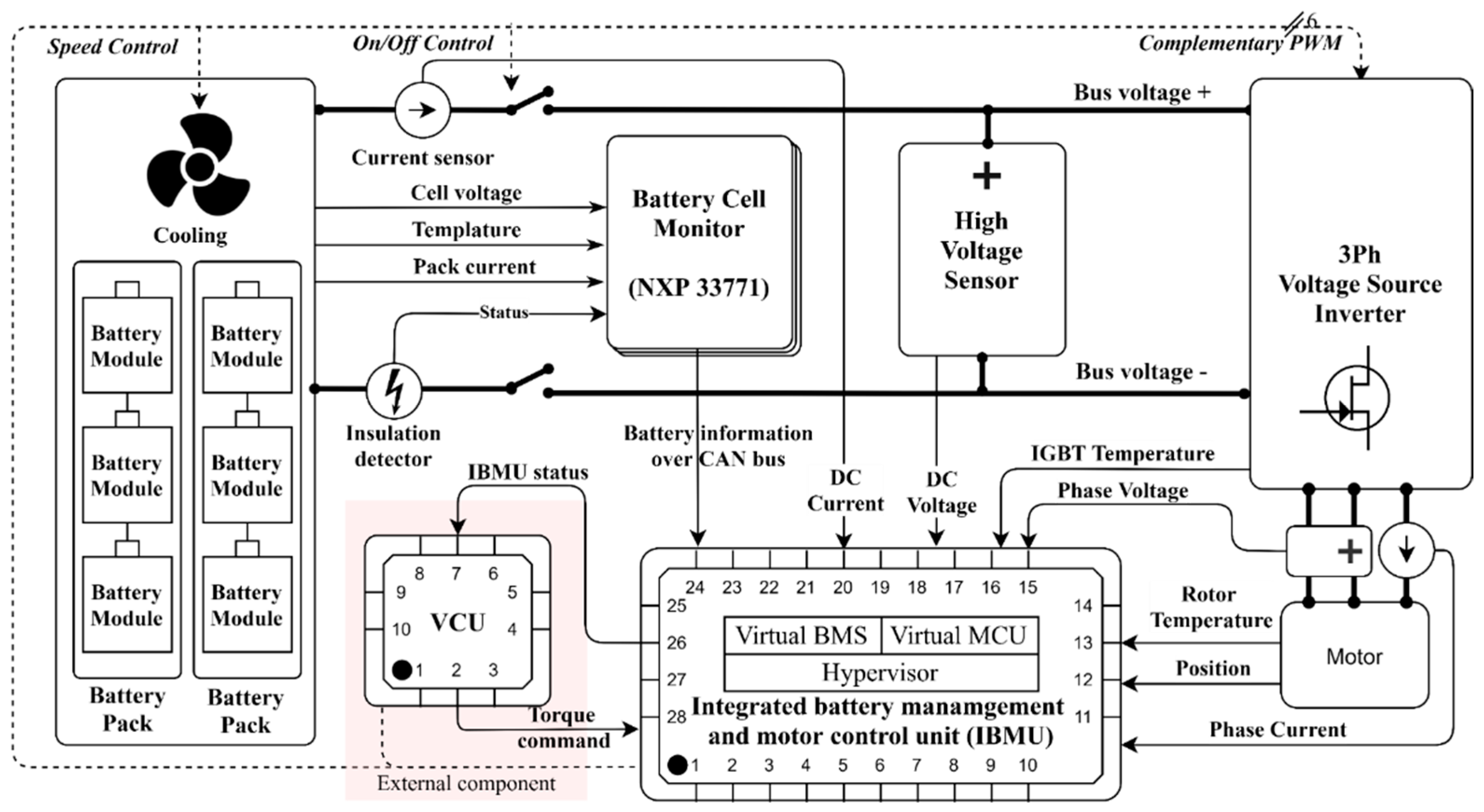
The powertrain system controllers of most electric vehicles include the vehicle controller unit (VCU), motor controller unit (MCU), and battery management system (BMS), connected via control area network (CAN) [3]. Among them, BMS and MCU are responsible for generating the vehicle propulsion like the traditional internal combustion engine system. The main function of BMS is to monitor and calculate the state of charge (SoC), state of health (SoH), and state of power (SoP) of the battery pack, equalize the battery cell voltage [4,5,6,7,8], and further ensure its safety through relying on the DC bus current sensor, the battery cell voltage sensor, and the temperature sensor [9,10,11], while Bukhari shows that the MCU performs the related propulsion control based on the battery status, phase current sensor, rotor position sensor, and temperature sensor [12]. Both BMS and MCU systems strongly rely on the signals of the sensors, and any fault may cause both systems the unexpected behaviors [13]. Therefore, the mechanisms of effective sensor fault detection and isolation are much required.

The common MCU faults include damage or short circuit of power switching transistor and sensor anomalies. The extended Kalman filter (EKF) can be used to calculate the residual of the sensor, effectively avoid system failure caused by single sensor fault [14,15] Furthermore, the additional current sensor can be used to reconstruct the phase current and to achieve multiple fault tolerance of the motor controllers [16]. Some research has used deep long short-term memory as the residual generator and the random forest (RF) algorithm as the fault classifier to perform early fault diagnosis of wind turbines [17]. The advantage of this method is not necessary to know the physical model of the system. In addition, the fast Fourier transform can be used to obtain the characteristics of the signal, and further construct Bayesian networks to detect the faults of the inverter [18].

The common BMS fault can be classified into internal and external faults [19,20]. Internal faults include the characteristic changes of battery due to the overcharge, over-discharge, overheating, thermal runaway, electromagnetic interference induced failure [21], and other behaviors, while the external faults consist of the abnormalities in the cooling system, wiring, or sensors. Many studies have adopted the model-based method to detect sensor faults.

A sliding mode observer based on electrical design is used to detect voltage, temperature, and current sensor failures [22]. Coulomb counting based and unscented Kalman filter (UKF) can help to estimate the SoC of each battery cell, and calculate the residual between the two to further find the sensor fault in the battery pack [23]. The recursive least squares method was used to estimate the equivalent model and adapt common change-point algorithm to detect anomalies in voltage and current sensors [24].

In general, fault detection mechanisms can be classified into three methods: residual generation by model-based method [14,15,23,25], data driven based method [17,18,26,27,28,29,30], and hybrid method [16,23].

The vast majority of researchers have focused on the fault detection mechanism for one single sensor, and the generation of estimated signals through other normal sensors to achieve fault tolerance. However, it is common to encounter multiple faults at the same time in vehicles due to the common cause failure (CCF). For example, as two phase current sensors often share the same set of power supplies, the power supply failure can cause their abnormal situation simultaneously. Hence, maintaining the operating characteristics of the system in this situation becomes a major challenge.

In addition, the residual generation by the model-based method can effectively detect faults of the sensors, but the premise is to rely on the accurate model parameters to ensure the system reliability. Although the motor parameters cannot generate too significant changes throughout the product life cycle, the manufacturing tolerances can pose the great challenges in obtaining parameters. Thus, using the model-based fault detection mechanism may cause improper results. This further leads to greater challenges for model-based diagnosis techniques. On the contrary, the use of redundant sensors, do not rely on accurate models. However, it is quite rare to use redundant sensors in the controllers of vehicles, due to cost factors.

In this study, a new integrated battery management and motor control system (IBMS) is proposed. Under the premise of not increasing the costs of the sensors, the integrated system can help mutual system sensors to generate redundant signals and to further reshape the output through the machine learning. The proposed IBMS system can realize the requirement of continuous operation and verify in the MIL system. The main contribution of this work is to propose the new architecture and algorithm of the powertrain, and to constitute the mutually redundant sensors of BMS and MCU from the system aspect. As a result, the powertrain system will effectively avoid the failure when the sensors of these two sub-systems are faulty.

2. Fail-Operational Architecture

2.1. System Overview

The proposed architecture for IBMS is show in Figure 1, where the virtual BMS and MCU are running on the high-performance controller, called integrated battery management and motor control unit (IBMU). Within this architecture, the user’s pedal commands are converted into torque by the external VCU and then fed into the IBMU through CAN.

The battery system consists of several battery packs, contained within each pack are several battery modules connected to battery cell IC controller. Each chip provides the measurement signals for the IBMU, while the battery packs are arranged in parallel through the power distribution unit. Based on the values of cell voltage and pack current, the SoC and SoP are calculated by the virtual BMS and provided to the virtual MCU. Finally, the virtual MCU performs the current closed-loop control, torque command, phase current, and rotor position.

The IBMS builds the important and complementary sensors through integrating BMS and MCU, so that the virtual system can still operate under the condition of some sensor fault. For example, the integration of heterogeneous signals and machine learning arbitration helps the system to continue operation by allowing the tolerance of multiple signal faults. This is done by (1) having the battery management system requiring to take the direct current (DC) bus current signal and (2) having the cell voltage signal as the input being used to estimate the battery SoC, and (3) having the motor controller taking the phase current signal and the DC bus voltage signal as the input of the field-oriented control (FOC) algorithm. In this setup, the DC bus current and phase current can be converted by special sampling and calculation to achieve fail-operation. As indicated in

Table 1. Functional hazard analysis.

Sensor Name	Main Function	Malfunction	Vehicle Effect
Phase current	Close loop current control	FOC abnormal	Unintended acceleration and deceleration
Rotor position	Phase current coordinate transformation and rotor speed estimation	FOC abnormal	Unintended acceleration and deceleration
DC bus voltage	PWM modulation index calculation and Battery status estimation	PWM width deviation	Unintended acceleration and deceleration Battery cell overcharge or overdischarge
DC bus current	Battery status estimation	Incorrect SoC and SoP	Battery cell overcharge or overdischarge
Battery cell voltage	Battery status estimation and voltage balancing	Incorrect SoC and SoP	Battery cell overcharge or overdischarge

, it shows that the main sensors of BMS and MCU and the hazard caused by their faults, because these main sensors can directly affect the vehicle.

2.2. Functional Hazard Analysis

Figure 2 is the IBMS architecture fault tree analysis, of which the solid line is the failure relationship between the original BMS and the MCU system. It can be seen that any single sensor fault will cause the unexpected behaviors of the system before the introduction of the architecture and algorithm. The dotted line emphasizes the analysis result of redundant signals after integrating the BMS, MCU, and proposed algorithm, especially the AND gate in the failure path can effectively avoid the single point of failure (SPOF) and CCF. Under the premise of not changing the component failure rate, the new architecture can reduce the failure rate of about one order of magnitude. For example, assume that the probability of failure of each sensor is 1 × 10⁻³ (P1–P6), and the controller is 1 × 10⁻⁴ (P7). In the original architecture, the probability of field oriented control module failure event is 2.997 × 10⁻³, while the proposed architecture is 3.029 × 10⁻⁴ [31]. In this study, two strategies, the use of heterogeneous sensors and the use of different algorithms, were adopted to avoid system failures caused by CCF.

3. The Proposed Approach

Figure 3 is a block diagram of the IBMU algorithm, which can be divided into four blocks: (a) Control signal fusion module, responsible for signal arbitration and redundant generation; (b) motor control module, responsible for the operation of FOC algorithm; (c) battery status monitor module, responsible for monitoring the status of the battery such as SoH, SoC, SoP, and other indicators, battery balance, as well as the connection of relays; (d) supporting module responsible for thermal management, communication, signal conversion, IO control, and implementing emergency measures.

The fault detection process includes several steps: (1) The supporting module acquires the raw signal and divides the signal into two groups. The first group includes the DC bus current signal, phase voltage signal, cell voltage signal, and pack current signal and the second group includes the phase current signal, rotor position signal, DC bus voltage signal, and phase voltage signal; (2) the first group will generate reconstructed signals based on signal recombination or sampling; (3) the second group will use a model-based approach to generate estimated signals; (4) the three sets of signals are used by random forest classifier to find the source of the failure sensor.

3.1. Motor Control Module

Motor control module uses the FOC algorithm to control the three-phase AC motor. FOC allows the separate control of the magnetic flux and torque. To simplify the motor model, FOC uses Park and Clark transformations to perform coordinate conversion of the three-phase current as in Equations (1)–(4), where $i_d$ is the flux control current, $i_q$ is the torque control current, $i_a i_b$ are the phase current and ${\theta }_r$ is the rotor position.

$$i_{\alpha }=i_a$$

(1)

$$i_{\beta }=\frac{1}{\sqrt{3}}{i}_a+\frac{2}{\sqrt{3}}{i}_b$$

(2)

$$i_d=i_{\alpha }\cos {\theta }_r+i_{\beta }\sin {\theta }_r$$

(3)

$$i_q=-i_{\alpha }\sin {\theta }_r+i_{\beta }\cos {\theta }_r$$

(4)

After the coordinate conversion, the circuit model of the permanent magnet motor can be expressed as in Equations (5) and (6), where the back electromotive forces $e_d$ and $e_q$ are related to the generated flux. In permanent magnet motor, most magnetic field is generated by the magnet installed on rotor, and the generated magnetic flux is a fixed value. In (7) ${\lambda }_f$ is the magnetic flux generated by the magnet, while the stator magnetic flux ${\lambda }_d$ and ${\lambda }_q$ are related to the current, as shown in Equations (7) and (8). Equations (9) and (10) expressed the back electromotive forces of d-q axis as the rotor speed multiplies with the magnetic flux. PMSM torque equation is shown in (11), in which two PID are used to regulate $i_d{i}_q$ to control of the motor torque [32].

$$v_d=R_s{i}_d+L_d\frac{d{i}_d}{dt}-e_d$$

(5)

$$v_q=R_s{i}_q+L_q\frac{d{i}_q}{dt}+e_q$$

(6)

$${\lambda }_d=L_d{i}_d+{\lambda }_f$$

(7)

$${\lambda }_q=L_q{i}_q$$

(8)

$$e_d={\omega }_r\times {\lambda }_d$$

(9)

$$e_q={\omega }_r\times {\lambda }_q$$

(10)

$$T_e=\frac{3}{2}{n}_p\times {\lambda }_f{i}_q+\left(L_d-L_q\right)i_d{i}_q$$

(11)

where $v_d v_q$ are the d-q axis stator voltage, $R_s$ is the stator resistance, ${\omega }_r$ is the rotor angular speed and $L_d L_q$ are the d-q axis inductance.

3.2. Battery Status Monitor Module

This study mainly focuses on the impact of sensor fault on SoC and SoP, in which SoC estimates the remained mileage and SoP directly affects the power output. The SoC estimation method can be divided into eight types [9], of which Coulomb counting and electrical model-based estimation is a relatively mature and widely used algorithm. The most common SoC estimation method is to use Coulomb counting indicated in Equation (12), where $\mathrm{SoC}\left(t_0\right)$ is the initial value of SoC, $C_Q$ is the rated capacity, $I_{dc}$ is the current on the DC bus, and $I_{loss}$ is the chemical loss of the battery itself.

With the measured output current, the battery capacity can be obtained by accumulating the electric charge. This method is required to accurately measure the battery current, obtains the initial SoC, and conducts the integration for charging and discharging current during the process. While the initial state of the SoC can be obtained through the battery usage history or the open circuit voltage (OCV) method. Another common SoC estimation method relies on the EKF [33,34] of which state models are shown in Equations (13) and (14), where w is the system noise, v is the measurement noise. These two vectors are uncorrelated and zero-mean vector.

$$\mathrm{SoC}\left(t\right)=\mathrm{SoC}\left(t_0\right)+\frac{1}{C_Q}{{\displaystyle \int }}_{{\mathit{t}}_0}^t\left(I_{dc}-I_{loss}\right)dt$$

(12)

$$\dot{\mathit{x}}=f\left(\mathit{x},\mathit{u}\right)+\mathit{w}$$

(13)

$${\mathit{y}}_{\mathit{k}}=h\left(\mathit{x},\mathit{u}\right)+\mathit{v}$$

(14)

The battery equivalent circuit model as show in Figure 4 [35,36,37] is used to estimate the state of the cell, with the internal state from SoC. The accuracy of EKF, based SoC algorithm, depends on its equivalent circuit model and the related parameters, including internal resistance $R_0$, diffusion resistance $R_n$, and diffusion capacitance $C_n$ as shown below.

Higher-order models can achieve better fitting effects, but require more computing resources. This research adopts three RC pairs to establish the model (15), of which $\mathit{x}$ is the selected state vector, including the SoC and voltage of RC pair. The input vector $\mathit{u}$ is the change in the DC bus current due to charging or discharging, and the output vector $\mathit{y}$ is the cell voltage, it can be obtained by adding up the voltage of OCV and the voltage of RC pair. The behavior model of the battery is described in Equation (16).

The EKF operation includes two steps, the prediction and correction steps. The prediction step is to calculate the predicted state ${\widehat{\mathit{x}}}_k^{-}$, and the predicted covariance matrix ${\mathit{P}}_k^{-}$, as shown in Equations (17) and (18), where ${\mathit{T}}_s$ is the sampling period of EKF and $F$ is the system Jacobian matrix. The second step is to update the results from the predicted state. First, it calculates the Kalman gain ${\mathit{K}}_k$ using Equation (19). Next, it corrects the values of ${\widehat{\mathit{x}}}_k^{-}$ from (17) by (20) and update the covariance matrix ${\mathit{P}}_k^{-}$ from (18) by (21), where $\mathit{H}$ is the measurement Jacobian matrix.

$$\begin{gathered} \mathit{x}={\left[\begin{array}{cccc}SoC& V_1& V_2& V_3\end{array}\right]}^T \\ \mathit{u}=\left[I_{dc}\right], \mathit{y}=\left[V_{cell}\right] \end{gathered}$$

(15)

$$\begin{gathered} \left[\begin{array}{c}\dot{SoC}\\ {\dot{V}}_1\\ {\dot{V}}_2\\ {\dot{V}}_3\end{array}\right]=\left[\begin{array}{c}\frac{I_{dc}}{C_Q}\\ \frac{-V_1}{R_1{C}_1}+\frac{I_{dc}}{C_1}\\ \frac{-V_2}{R_2{C}_2}+\frac{I_{dc}}{C_2}\\ \frac{-V_3}{R_3{C}_3}+\frac{I_{dc}}{C_3}\end{array}\right] \\ {V}_{cell}=V_{ocv}+I_{dc}{R}_0+V_1+V_2+V_3 \end{gathered}$$

(16)

$${\widehat{\mathit{x}}}_k^{-}={\widehat{\mathit{x}}}_{k-1}+T_{s}f\left({\widehat{\mathit{x}}}_{k-1},{\mathit{u}}_k\right)$$

(17)

$${\mathit{P}}_k^{-}={\mathit{P}}_{k-1}+\mathit{F}{\mathit{P}}_{k-1}{\mathit{F}}^T+\mathit{Q}$$

(18)

$${\mathit{K}}_k={\mathit{P}}_k^{-}{\mathit{H}}^T{(\mathit{H}{\mathit{P}}_k^{-}{\mathit{H}}^T+\mathit{R})}^{-1}$$

(19)

$${\widehat{\mathit{x}}}_k={\widehat{\mathit{x}}}_{k-1}^{-}+{\mathit{K}}_k\left[{\mathit{y}}_k-h\left({\mathit{x}}_k\right)\right]$$

(20)

$${\mathit{P}}_k={\mathit{P}}_k^{-}-{\mathit{K}}_k\mathit{H}{\mathit{P}}_k^{-}$$

(21)

With the DC bus current sensor, the Coulomb counting method can estimate the SoC of the battery easily, but the accumulation of integration errors and different usage situations of battery may lead to significant errors. By measuring cell voltage and DC bus current, EKF based SoC algorithm can timely correct the errors of the initial value and suppress noises. In this study, both methods are adopted and switch based on the condition of the sensor. Being the another battery status indicator, SoP has a more direct impact on the system, which evaluates the available output power of the battery under safe conditions [8]. The torque output of the powertrain system can be adjusted according to this number, especially the wrong SoP can cause the unexpected acceleration and deceleration of the vehicles. The most common situation is when the motor driver uses more power than that is available can greatly drop the battery voltage and trigger the low voltage protection mechanism to cause the discontinuity of propulsion. The calculation of SoP is closely related to the degree of battery aging, the ambient temperature, and the use situation. Feature lookup table is the most extensive estimation method. In this study, we mainly build SoP into a three-dimensional table and further calculate the output limit of current based on the battery temperature, SoC and SoH as show in Figure 5.

3.3. Control Signal Fusion Module

The control signal fusion module of fault-tolerant system relies on the heterogeneous signal reconstruction and signal estimation to build the corresponding fusion algorithm that can detect and isolate multiple faults in the IBMS system. As shown in Figure 6, the sensor fusion module includes three sub blocks: (a) signal estimation, (b) signal reconstruction, and (c) signal arbitration blocks.

The signal estimation block uses the phase current signal and the extended Kalman filter to predict the phase current and rotor speed signal. The signal reconstruction block is responsible for the rebuilding phase current signal through the DC bus current sensor and the pulse width modulation (PWM) status, and uses the line voltage sensor and back electromotive force to calculate the rotor speed. The DC bus voltage can be obtained by calculating the sum of the single cell voltage, while the DC bus current can be acquired by calculating the sum of the battery pack current signals or reconstructed by calculating phase current and PWM status.

Although both blocks can output current, voltage, and rotor speed signals, the signal reconstruction block focuses on converting real measurement signals into target data through calculation, while the estimation block concentrates on using the motor and battery model to predict the signal. The processing mechanisms of the signal reconstruction and signal estimation can effectively make the operation normal even when facing the CCF. On the other hand, the signal arbitration module plays the role of the final decision-making. By collecting a large amount of data and training the random forest model, it can help determine the possible failure factors of the system, and further reconfigure the control signal through the finite state machine.

3.3.1. Reconstruction Block

DC bus current, phase voltage, battery cell voltage, and battery module current can be used to reconstruct $I_{dc}^{recon}$, $V_{dc}^{recon}$, and ${\omega }_r^{recon}$, where $V_{dc}^{recon}$ and $I_{dc}^{recon}$ and can be obtained from Equations (22) and (23) by summing the cell voltage and the module current respectively, while the value of ${\omega }_r^{recon}$ is the result of calculating the zero-crossing frequency of the phase voltage.

$$V_{dc}^{recon}={\displaystyle \sum }_{i=1}^n{V}_{cell\left(n\right)}$$

(22)

$$I_{dc}^{recon}={\displaystyle \sum }_{i=1}^n{I}_{pack\left(n\right)}$$

(23)

Finally, the phase current $i_a^{recon}$ and $i_b^{recon}$ are rebuilt utilizing DC bus current [38,39,40]. These studies showed how to utilize the single current sensor to rebuild the phase current.

Table 2. Current flow paths table.

Sectors	V0	V1	V2	V3	V4	V5	V6	V7
$I_{dc}$	0	$+i_a$	$-i_c$	$+i_b$	$-i_a$	$-i_c$	$+i_b$	0

indicates the relationship between the DC current and the AC current for the switched PWM.

When the PWM is switched into V0 and V7 sector, $I_{dc}$ has no current. When the PWM operates in V1 sector, the measured DC bus current flows into $S_a$ and out from $S_b^{\prime }$ and $S_c^{\prime }$, the measured DC bus current is equal to the signal of the phase A current, as shown in the red dotted line of Figure 7a. When the PWM operates in V2 sector, the measured DC bus current is a negative phase C current as shown in the green dotted of line Figure 7b. And the phase current signal can be reconstructed based on this logic.

3.3.2. Estimation Block

Estimation block consists of three subunits, including the DC voltage estimation unit, the DC current estimation unit and the phase current and rotor speed estimation, which can be used to produce the estimated control signals shown in Figure 8.

The DC voltage estimation unit uses torque and motor speed to calculate the overall system power, as shown in (24), of which $T_e$ is the torque estimation equation in (11). To obtain the value of DC voltage, (25) is employed. Note that ${\eta }_{sys}$ is the system efficiency of the controller and the motor operations in different situations. ${\eta }_{sys}$ is various for different speeds and torques. Therefore, it is necessary to first build the efficiency table when using this method.

$$V_{dc}^{recon}={\displaystyle \sum }_{i=1}^n{V}_{cell\left(n\right)}$$

(24)

$$I_{dc}^{recon}={\displaystyle \sum }_{i=1}^n{I}_{pack\left(n\right)}$$

(25)

The DC current estimation unit assumes that the input power $V_{dc}{I}_{dc}$ multiplies by the system efficiency ${\eta }_{sys}$ to get the output power as shown in (26), where $V_{pha-a}$, $V_{pha-b}$, and $V_{pha-c}$ are the root-mean-square values of the three-phase voltages. The amplitudes of PWM can be expressed as in (27)–(29), where $S_a$, $S_b$ and $S_c$ are the duty of PWM. Substituting (27)–(29) into (26), the DC bus current $I_{dc}$ is shown in (30).

$$V_{dc}{I}_{dc}{\eta }_{sys}=i_a{V}_{pha-a}+i_b{V}_{pha-b}+i_c{V}_{pha-c}$$

(26)

$$V_{pha-a}=S_a\times \frac{1}{\sqrt{3}}{V}_{dc}\sin \left(\omega t\right)=v_A\times \frac{1}{\sqrt{3}}{V}_{dc}$$

(27)

$$V_{pha-b}=S_b\times \frac{1}{\sqrt{3}}{V}_{dc}\sin \left(\omega t+\frac{2\pi }{3}\right)=v_B\times \frac{1}{\sqrt{3}}{V}_{dc}$$

(28)

$$V_{pha-c}=S_c\times \frac{1}{\sqrt{3}}{V}_{dc}\sin \left(\omega t+\frac{2\pi }{3}\right)=v_C\times \frac{1}{\sqrt{3}}{V}_{dc}$$

(29)

$$I_{dc}=\frac{1}{\sqrt{3} {\eta }_{system}}\left(i_a{v}_A+i_b{v}_B+i_c{v}_C\right)$$

(30)

In phase current and rotor speed estimation unit, the EKF algorithm is utilized to generate the estimated phase current and rotor speed. In Equation (31) $x$ is the selected state vector, which includes the magnetic flux of the d-q axis, the rotor speed, and the rotor degree. In Equation (31), the input vector is the voltage and the output part is the phase current, where the state matrix $f$, the measurement matrix h, the system Jacobian matrix F, and the measurement Jacobian matrix H are shown in Equations (32)–(35), respectively. The EKF algorithm can estimate the best value of $\mathit{x}$ state, and further estimate the phase current, based on Equation (33).

$$\mathit{x}=\left[\begin{array}{c}{\lambda }_d\\ {\lambda }_q\\ \omega \\ {\theta }_r\end{array}\right] \mathit{u}=\left[\begin{array}{c}{v}_d\\ v_q\end{array}\right] \mathit{y}=\left[\begin{array}{c}{i}_a\\ i_b\end{array}\right]$$

(31)

$$\mathit{f}=\left[\begin{array}{c}-\frac{R_s}{L_d}{\lambda }_d+{\omega }_r{\lambda }_q+\frac{R_s}{L_d}{\lambda }_f+v_d\\ -{\omega }_r{\lambda }_d+\frac{R_s}{L_q}{\lambda }_q+v_q\\ 0\\ {\omega }_r\end{array}\right]$$

(32)

$$\mathit{h}=\left[\begin{array}{c}\frac{{\lambda }_d-{\lambda }_f}{L_d}\cos {\theta }_r-\frac{{\lambda }_q}{L_q}\sin {\theta }_r\\ \frac{{\lambda }_d-{\lambda }_f}{L_d}\left(\frac{\sqrt{3}}{2}\sin {\theta }_r-\frac{1}{2}\cos {\theta }_r\right)-\frac{{\lambda }_q}{L_q}\left(\frac{1}{2}\sin {\theta }_r+\frac{\sqrt{3}}{2}\cos {\theta }_r\right)\end{array}\right]$$

(33)

$$\mathit{F}=\frac{\partial \mathit{f}}{\partial x}=\left[\begin{array}{cccc}\frac{-R_s}{L_d}& {\omega }_r& {\lambda }_q& -v_{\alpha }\cos {\theta }_r+v_{\beta }\sin \theta \\ -{\omega }_r& \frac{-R_s}{Lq}& -{\lambda }_d& v_{\alpha }\cos {\theta }_r-v_{\beta }\sin \theta \\ 0& 0& 0& 0\\ 0& 0& 1& 0\end{array}\right]$$

(34)

$$\mathit{H}=\frac{\partial \mathit{h}}{\partial x}=[\begin{array}{cccc}\frac{1}{L_d}\cos {\theta }_{\mathit{r}}& -\frac{1}{L_q}\sin {\theta }_{\mathit{r}}& 0& -\frac{{\lambda }_d-{\lambda }_f}{L_d}\sin {\theta }_r-\frac{{\lambda }_q}{L_q}\cos {\theta }_r\\ \frac{1}{L_d}\left(\frac{\sqrt{3}}{2}\sin {\theta }_r-\frac{1}{2}\cos {\theta }_r\right)& \frac{1}{L_q}\left(\frac{1}{2}\sin {\theta }_r+\frac{\sqrt{3}}{2}\cos {\theta }_r\right)& -{\lambda }_d& \frac{{\lambda }_d-{\lambda }_f}{L_d}(\frac{\sqrt{3}}{2}\cos {\theta }_r-\frac{1}{2}\sin {\theta }_r)+\frac{{\lambda }_q}{L_q}(\frac{1}{2}\cos {\theta }_r-\frac{\sqrt{3}}{2}\sin {\theta }_r\end{array}]$$

(35)

3.3.3. Signal Arbitration

After the process of signal reconstruction and signal estimation, multiple sets of reference signals are obtained. The essence of the random forest (RF) classifier, which we used for arbitration, is a mixture of decision trees, bagging, and random concepts. Compared to traditional decision trees, the random forest algorithm relies on Bootstrap in order to obtain several databases and further build into a decision tree.

To form the required computing resources and performances, the results from the RF method [41] are compared with two machine learning algorithms: decision tree and support vector machine (SVM). Given that the classified content is a time series, when generating the training model dataset, time domain features should also be extracted to take the coefficient of variation, mean and peak to peak, residuals of the original signal, reconstructed signal, and estimated signal as the part of the training dataset in addition to using the raw data.

4. Evaluation of the Proposed Approach

To quickly train the classification model and test different fault scenarios, this work uses the MIL system to verify the proposed architecture and algorithm [42].

4.1. Evaluation Environments

Figure 9 shows the construction of the MIL system, including the offline modeling and real-time in the loop simulation. A sufficiently accurate model should be essential to make MIL verification closer to the actual verification. In this study, the battery model 120155250N manufactured by AMITA and 50 KW PMSM motor were selected as modeling targets. The way to build the battery model is based on what Huria proposed [43]. The motor flux model is able to be completely established by measuring the three-phase voltage and current [44]. After the offline parameters are fully identified, the plant models of the battery and the motor can be placed in the real-time simulator, and the IBMU algorithm, proposed in this work, is applied in the virtual microcontroller. The high-fidelity physical plant model and virtual microcontroller can be effectively connected through the internal communication protocol or share memory. Because all the sensor signals are generated by the real-time simulator and plant model, the abnormal situation of the sensor can be easily inputted into the MIL system, in which the quick emulator (QEMU) can help to simulate the virtual microcontroller, with the set Central Processing Unit (CPU) frequency at 1000 MHz.

4.2. Model Training and Deployment

The motor and battery have different bandwidth responses, hence the speed of executing error diagnosis is also different. In order to reduce the load of the controllers, the fault classification model has been divided into two parts. The main classification model has a total of 75 input signals, including 5 measured signals, 11 estimated or reconstructed signals, 11 residual values, and 48 feature extraction variables. All features would first be normalized to ensure that the data is between 0 and 2, and the sensor status has five types; that is, the normal state, no signal, bias, stuck, and intermittent fault for encoding.

The proposed architecture is simulated through Simulink and by changing the state of the sensor to generate the variant test data sets and labeling data sets, as shown in

Table 3. Sensor fault scenario and output label encoding.

Scenario Description	${\mathit{i}}_{\mathit{a}}$	${\mathit{i}}_{\mathit{b}}$	${\mathit{\theta }}_{\mathit{r}}$	${\mathit{V}}_{\mathit{d}\mathit{c}}$	${\mathit{I}}_{\mathit{d}\mathit{c}}$	${\mathit{V}}_{\mathit{c}\mathit{e}\mathit{l}\mathit{l}\mathit{l}}$	${\mathit{I}}_{\mathit{p}\mathit{a}\mathit{c}\mathit{k}}$	Output Label
Normal	5	5	5	5	5	5	5	5555555
Loss of phase A current signal	4	5	5	5	5	5	5	4555555
Phase A current sensor has a bias fault	3	5	5	5	5	5	5	3555555
Loss of phase A and B current signal	4	4	5	5	5	5	5	4455555
Loss of phase A current signal and DC bus voltage sensor has a bias fault	4	5	5	3	5	5	5	4553555
Loss of DC bus current signal	5	5	5	5	4	5	5	5555455
Loss of battery cell voltage signal	5	5	5	5	5	4	5	5555545
Loss of DC bus voltage signal and phase A current sensor has a signal bias fault	3	5	5	4	5	5	5	3554555

. In each situation, 20,000 data are obtained, and are used to train three classification models of decision tree, random forest, and SVM. In the decision tree part, it relies on all the features and takes Gini index as the split, in order to better limit 60 of the maximum number of splits. During the process of training random forest, it takes 20 classification trees and all features as the upper limits, while SVM uses the linear kernel to train the model and classify errors.

The secondary classification model is used to locate the ill-functioned integrated circuit (IC). The cell voltage is usually measured by a specific battery cell controller IC. For example, a single MC33771B manufactured by NXP Semiconductors can be used to measure the voltage of up to 14 cells. In this study two groups of 84S3P battery packs are selected, that means the IBMU needs at least 12 ICs to measure all cell voltage signals. The aforementioned main model is responsible for confirming the IC state, while the secondary model is responsible for fault detection from 12 ICs.

4.3. Measure for Implementation

The architecture proposed by this study includes the signal fusion algorithm using machine learning, motor control algorithm, battery status monitor algorithm, as well as other logical operations or drivers with the lower computational load. In the past, due to the limitations of chip performance, there were fewer chips that could meet the functional safety, as well as simultaneously control the motor and estimated battery status. According to the related experiments, TMS570 ARM Cortex R4 chip manufactured by Texas Instruments single core 160 Dhrystone million instructions executed per second (DMIPS) can complete MCU control roughly for 60 μs of computing time without specific hardware acceleration requirements. Under the control system of 10 kHz PWM frequency, the CPU load reached nearly 70% and was unable to integrate other algorithms. However, in recent years, the architecture of vehicle electronic systems has gradually evolved from the central gateway architecture to the domain controller architecture. Thus, the high-performance chips suitable for power systems have begun to appear in the market, such as the S32P series chips launched by NXP which can own the computing power of 6000 DMIPS. It can be said that the emergence of domain controller realizes the architecture proposed by this research. Figure 10 is the algorithm flow chart of the IBMU.

Figure 11 is the execution timing of each task, and the highest priority interrupt can execute once every 100 μs. Task T2 is triggered by this interrupt which is responsible for the calculation of FOC algorithm and timely outputting the results to the hardware circuit. The second highest priority interrupt can execute once every 200 μs. Task T1 is triggered by this interrupt which is responsible for generating redundant signal.

Tasks T3 and T4 perform SoC estimation every 10 ms and 100 ms, respectively. As each EKF estimation can only be conducted for one battery, the whole SoC estimation time actually requires 840 ms, and SoP can be performed after the calculation of all batteries. Task T5 is executed at the speed of 20 ms, which is mainly responsible for the main fault classification and invoke fault handler after detecting the fault. Task T6 mainly performs the second level classification, and its goal is to find the faulty measurement IC.

Table 4. Average task execution time and CPU load.

Task	Execution Time	CPU Load
T1	140~150 μs	75%
T2	35~40 μs	40%
T3	4.1~4.3 ms	43%
T4	10~12 μs	0.0001%
T5	14~15 ms	75%
T6	150~200 μs	NA

summarizes the evaluation of the utilization rate of each task. This research mainly adopts the QEMU ARM Cortex A9 1000 MHz simulator provided by MathWorks for testing, and the computing power of this simulation chip is about 2500 DMIPS/Core. The overall CPU load is around 233%, which means that the CPU needs at least 6000 DMIPS or higher computing power to cover all task execution.

4.4. Comparison of Results

Figure 12 it indicates that the response for each sensor is healthy, which can be used as a baseline for comparison of other experiments. In this simulation, the motor continuously outputs 100 Nm of torque as a load and continuously discharges the battery for 10 s. The referred SoC and Torque used in Figure 12a are consistent with the estimated results. The raw sensor data, reconstructed data and estimated data of the sensors in Figure 12b–d, are all consistent. Specifically, the residual is also within the tolerance range. This means that both the estimated signal and the reconstructed signal can replace the raw sensor signal. The impact of each sensor fault, and the required time to restore the system will be introduced later.

4.4.1. Phase Current Sensor Fault

Figure 13 shows the system response after losing the phase A current sensor signal. Since the frequency of motor control task is much higher than the frequency of fault detection task, the system will temporarily lose control after the fault is injected at 0.05 s and cause an unstable in the torque output of the motor. When the fault is diagnosed at 0.076 s, one can switch the FOC control algorithm input signal from the raw current sensor signal to the reconstructed sensor signal and make the system return to stability at 0.085 s. In this research, diagnosis task is executed periodically, and the user can set the threshold of the phase current as the condition for task triggering.

4.4.2. DC Bus Voltage Sensor Fault

The torque output of motor is determined by current, the abnormality of voltage sensor does not directly affect the power output in most cases. However, in order to suppress the DC bus voltage ripple, the controller will acquire the dq axis command and then uses the voltage signal for compensation, which causes the torque command to be inconsistent with the output torque when the voltage sensor is abnormal. As shown in Figure 14, when the fault is injected into the voltage sensor signal at 0.05 s, the motor output will be lower than expected due to the voltage signal drift. In this case, the reconstructed DC bus voltage signal is based on the accumulation of the cell voltage; therefore, it will not be affected by the drift of the raw voltage sensor signal. However, the estimated DC bus voltage signal is calculated based on the Equation (11) and the output torque changes which indirectly lead to the accuracy of the estimated voltage signal. However, it is this signature that allows us to clearly diagnose signal drift faults. When the fault is diagnosed at 0.076 s, the voltage input of the motor control algorithm is switched to the reconstructed voltage signal, and the system is able to regain stability at 0.081 s.

4.4.3. DC Bus Current Sensor Fault

The fault of the DC bus current sensor will affect the estimation of the SoC. As the frequency of fault diagnosis is greater than the frequency of SoC calculation, most fault can be corrected timely. Figure 15 shows the impact caused by the worst case. The loss of DC bus current signal fault is injected at 5.99 s and the tasks of SOC estimation and main diagnosis are executed at 6 s. Since the diagnosis task takes 14 ms to complete, that is, the system can only diagnose the fault at 6.014 s, so the SOC estimation performed at the 6 s will be abnormal and cause deviation. When the system detects the fault at 6.014 s, it switches the input source of the SOC estimation signal from the raw DC bus current signal to the reconstructed DC bus current signal. Although the system has reconfigured the fault signal, the SOC estimation algorithm based on the Coulomb counter cannot correct the deviation caused by signal loss, the deviation is negligible.

4.4.4. Battery Cell Voltage Sensor Fault

The fault of the cell voltage mainly affects the estimation of the EKF based SoC and reconstructed DC bus voltage. In this work the battery pack has a total of 12 ICs for the voltage measurement of 86 cells. We can inject the fault at 6 s to make one of the measurement ICs invalid. Observing from Figure 16, this would cause the reconstructed voltage signal being lower than the original signal and would trigger the second fault classification model to determine the fault IC number for the isolation. In terms of SOC estimation, when a fault occurs, the SOC value will temporarily deviate from the reference value, but after the faulty ICs are isolated, the remaining ICs can still work properly, and the error will gradually converge. In this case, the system diagnoses the fault at 6.013 s and eliminate the system failure within 10 s.

4.4.5. Multiple Sensor Fault

Figure 17 is the system responses after the fault of losing two phase current sensors is injected at 0.05 s. After the fault is injected, the system cannot detect the fault immediately, so the torque output by the motor will be temporarily unstable. Since the frequency response of the vehicle is much lower than the electrical response, transient instability does not matter. A case of lost multiple signals would render the estimation algorithm based on EKF unable to work properly. At this time, the reconstructed phase current signal based on the DC current will be used as the input of the FOC algorithm. Therefore, when the system detects a fault at 0.076 s, it will switch the source of the control signal to the reconstructed current signal. Finally, the system can recover its stability at 0.85 s. Under the operation of multi-sensor fault, it is necessary to conduct the switching of multiple sets of signals. However, the direct switching multiple signal set will cause the system to take a longer period to restore stability and may even fail to converge. Under this circumstance, the PWM signal will be turned off shortly, and the source of the control signal will be reconfigured. Then the PWM sends the output signals again after signal reconfiguration.

In this architecture, the system can continue to operate even in the face of three sensor faults with only one exception where the current sensors of phase A, phase B, and DC bus all fault simultaneously. Nonetheless, most MCUs are designed with three current sensors as hardware overcurrent protection circuits. For MCU systems with three current sensors, a third current sensor can be used to restore the system.

Table 5. Evaluation result analysis.

Algorithm	Execution Cost	Accuracy	Fault sensor Name	Recover Time
Decision tree	0.21~0.23 ms	95.0%	Singe phase current sensor	~0.018 s
			Two phase current sensors	~0.017 s
			DC bus voltage sensor	~0.018 s
			DC bus current sensor	~0.11 s
			Battery cell voltage sensor	~4 s
Random forests	13.5~15.1 ms	97.9%	Singe phase current sensor	~0.031 s
			Two phase current sensors	~0.032 s
			DC bus voltage sensor	~0.032 s
			DC bus current sensor	~0.11 s
			Battery cell voltage sensor	~4 s
SVM	14.2~15.1 ms	98.0%	Singe phase current sensor	~0.031 s
			Two phase current sensors	~0.032 s
			DC bus voltage sensor	~0.032 s
			DC bus current sensor	~0.11 s
			Battery cell voltage sensor	~4 s

is the evaluated results through using different fault detection algorithms, of which the decision tree has the lowest execution cost with identifying 95% of faults in the first diagnosis cycle, while RF and SVM have the relatively higher execution cost and higher accuracy, compared to decision tree. The advantages of RF, compared to that of SVM, are that (1) the parameters of RF can be easily adjusted, (2) its memory required during the execution phase is lower, and (3) RF can effectively avoid the overfitting by introducing random features. Therefore, in an embedded system with limited resources, RF might be a better choice to achieve this specific purpose.

5. Conclusions

Model based fault tolerance system usually fails to the effective detection and isolation for the complex fault scenarios. Through integrating BMS, MCU, and using signal reconstruction, signal estimation, and signal arbitration methods, this work proposes a framework for sustainable operation. It can allow two systems to tolerate the faults of three sensors at the same time without increasing costs, and can further detect the fault types of sensors, including no signal fault, bias fault, stuck fault, and intermittent fault. Under the premise of not changing the component failure rate, the proposed IBMS can reduce the powertrain failure rate of about one order of magnitude. Three arbitration algorithms are utilized in the proposed system. Among them, the fault recognition rate of the RF algorithm is 97.4% in the first diagnosis cycle and higher accuracy will be obtained in the subsequent diagnosis cycle. The system recovery time is between 10 and 4000 ms, after the faults can be detected. Furthermore, this architecture can be achieved by chips with the floating point unit and computing power greater than 6000 DMIPS.