Article

DWT-LSTM-Based Fault Diagnosis of Rolling Bearings with Multi-Sensors

1
State Key Laboratory of Nuclear Power Safety Monitoring Technology and Equipment, China Nuclear Power Engineering Co., Ltd., Shenzhen 518172, China
2
College of Electrical and Power Engineering, Taiyuan University of Technology, Taiyuan 030024, China
*
Author to whom correspondence should be addressed.
Electronics 2021, 10(17), 2076; https://doi.org/10.3390/electronics10172076
Submission received: 22 July 2021 / Revised: 14 August 2021 / Accepted: 20 August 2021 / Published: 27 August 2021

Abstract

:
Bearings are widely used in many steam turbine generator sets and other large rotating equipment. With the rapid development of contemporary industry, there is a great number of rotating equipment in various large factories, such as nuclear power plants. As the core component of rotating machinery, the failure of rolling bearings may lead to serious accidents during the industrial production operation. In order to accurately diagnose the fault status of rolling bearings, a novel long short-term memory (LSTM) model with discrete wavelet transformation (DWT) for multi-sensor fault diagnosis is proposed in this paper. The main purpose of this paper is to use the DWT-LSTM model to diagnose the health of rolling bearings. Firstly, the DWT is used to obtain detailed fault information in both different frequency and time scales. Then, the LSTM network is employed to characterize the long-term dependencies hidden in the time series of the fault information. The proposed DWT-LSTM method makes full use of the advantages of feature extraction based on expert experience and deep network learning to discover complex patterns from a large amount of data. Finally, the feasibility and efficiency of the proposed method are illustrated by comparison with the existing methods.

1. Introduction

Modern industry is developing rapidly. Many factories, such as nuclear power plants, have already used large rotating equipment for industrial production [1]. Rolling bearings are widely used as main components in the rotating machinery and equipment of these factories. In practice, the health status of rolling bearings is directly related to the safety of equipment operation [2]. According to statistics, at least 40% of rotating machinery failures are caused by the damage of rolling bearings [3]. The inability of rolling bearings will lead to a severe failure of rotating machinery, which may endanger personal safety and causes property damage. Therefore, it is of great practical significance to diagnose the rolling bearing status effectively, promptly, and accurately.
The vibration signal contains important features that reflect the state of rolling bearing. Therefore, an efficient way of fault diagnosis is to extract features from the vibration signal generated by the rotating machinery in the running state [4]. In order to obtain useful information from the vibration signal that can reflect the operating status of mechanical equipment, various signal processing methods have been proposed, such as Fourier transformation [5], wavelet transformation [6], etc. However, the above traditional signal processing methods rely heavily on expert experience.
Due to the ability of deep feature self-learning, the deep learning method [7] has been widely used in fault diagnosis recently, which neither requires manual intervention nor relies on prior knowledge. Chiefly, auto-encoder (AE), convolutional neural network (CNN), and long short-term memory (LSTM) are utilized for fault diagnosis. In [8,9], AE was used to adaptively extract the fault features and classify the health condition of the rotating machinery. As an efficient algorithm for deep learning, CNN is also used for fault diagnosis of bearing [10]. In order to improve the diagnostic accuracy, a CNN fault diagnosis method with wide first-layer kernels was proposed in [11]. Considering the timing information of vibration signal, LSTM has been further employed to handle the long-term dependencies during the fault diagnosis [12,13]. In order to overcome the shortcomings of the shallow structure, a fault diagnosis algorithm based on stacked LSTM was proposed [14]. A new bearing fault diagnosis method, dense convolutional neural networks (ADCNN), was proposed in [15], which considers the temporal coherence of the data samples by combining dense convolution blocks and attention mechanisms. Multi-scale analysis of data helps to obtain richer features and improve fault diagnosis capabilities. In [16], Chen et al. used multi-scale CNN with different core sizes to extract different frequency features, which were sent to stacked LSTM and softmax to classify different fault states.
Since the vibration signal obtained from a single sensor may not contain full fault information, a CNN-based multi-sensor fusion method for the fault diagnosis of rotating machinery was proposed in [17]. In [18], the features of multiple sensors are extracted through the deep belief network (DBN), and the softmax classifier results are combined with the Debster–Shafer evidence theory to obtain accurate fault prediction. Multi-sensor input methods can get more fault characteristics, which can improve the accuracy of fault diagnosis.
Although the above end-to-end deep learning fault diagnosis methods have good performance, the diagnosis model is trained blindly only according to the obtained data, which leads to poor robustness. Professional knowledge and prior information are very important in the fault diagnosis process. Combining the advantages of professional experiences and deep learning technology, the complexity of fault diagnosis model can be effectively reduced, and the diagnosis accuracy can also be improved [19,20,21].
In this paper, in order to accurately identify different fault states of rolling bearing, a novel LSTM model with discrete wavelet transformation (DWT) for multi-sensor fault diagnosis is proposed. Sufficient fault information in different frequency bands on multiple scales can be obtained through the DWT, which can fully reflect the fault characteristics. The multi-scale data are fused as the input of the subsequent LSTM model to classify the health condition of the rolling bearing. The reliability and superiority of the proposed diagnosis framework are verified by comparison with other deep learning methods. Therefore, it can be concluded that the proposed algorithm has a higher fault diagnosis accuracy. The main contributions of the proposed fault diagnosis method are summarized as follows:
1
Multi-scale features from multiple sensors are fused in the proposed method for improving the model’s performance.
2
The professional knowledge is used in the entire algorithm design process, which can overcome the disadvantage of the blind training of the deep feature classification model.
3
Accurately identifies 10 different fault types by using the proposed DWT-LSTM method.
The rest of this article is structured as follows: Section 2 presents the proposed DWT-LSTM framework for fault diagnosis. The experimental data of a rolling bearing are presented in Section 3, where the validation and discussion of the DWT-LSTM model are also presented. Conclusions are presented in Section 4.

2. DWT-LSTM Fault Diagnosis Framework

The proposed DWT-LSTM framework architecture consists of five parts: multi-sensor data layer, DWT multi-scale layer, data fusion layer, LSTM layer, and the fault classification layer, which is shown in Figure 1.
The vibration signals from different sensors are collected first. Then, multi-scale vibration data are obtained through the DWT. The multi-scale information is fused as the input of the LSTM neural network for deep fault feature extraction. Finally, the softmax layer is used to classify the fault type by calculating the probability of different bearing fault states.
Compared with the LSTM model, the advantage of the proposed fault diagnosis scheme is that the advantages of professional knowledge and the deep feature extraction ability of deep learning are both considered. Furthermore, combined with the full fault information from multi-sensors, the accuracy and robustness of the fault diagnosis model can be improved significantly.

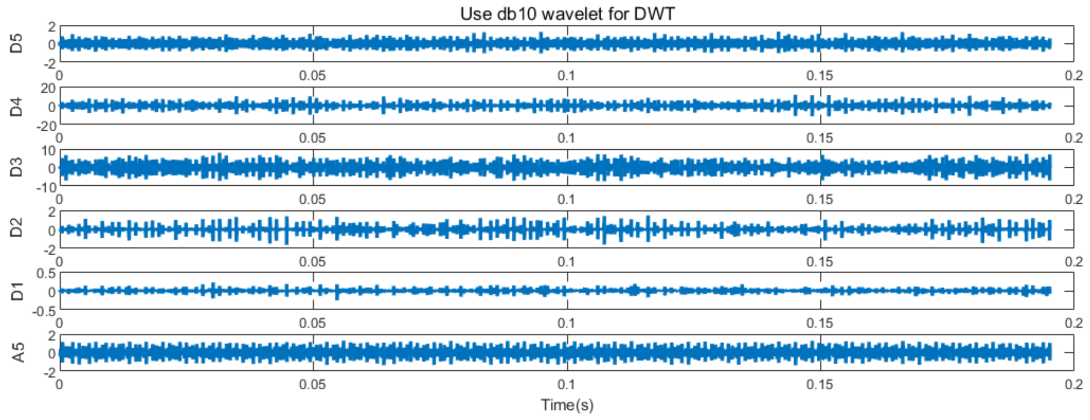
2.1. Discrete Wavelet Transform

In this section, DWT and multi-scale analysis are performed on the raw bearing fault data to obtain comprehensive and detailed fault information. DWT can reflect the data characteristics in both time and frequency. Through a series of expansion and translation operations, the DWT can gradually refine the signal on multiple scales. It decomposes the vibration signal into a number of sets, where each set is a time series of coefficients describing the time evolution of the signal in the corresponding frequency band.
DWT can be used in time–frequency analysis that decomposes a signal in both the time domain and frequency domain simultaneously [6]. Assuming that the original vibration signal in the time series collected by the ith sensor is denoted as X i ( t ) ( i = 1 , 2 , , N ) , the DWT can be defined as:
D W T ( j , k ) = 1 2 j + X i ( t ) ψ * t 2 j k 2 j d t ,
where 2 j and 2 j k represent the scale and translation parameters, respectively. j, k are integers. ψ represents the wavelet function. ψ * is the complex conjugate of ψ .
The multi-scale analysis of DWT is to perform multi-level DWT for the raw vibration signal to obtain the approximate coefficients and detail coefficients under j levels of different scales. The original signal X i ( t ) passes through a set of low-pass and high-pass filters to obtain low-frequency bands (approximations) and the high-frequency bands (details), respectively. Then, X i ( t ) can be defined as:
X i ( t ) = A j + l = 1 j D l ,
where A j represents the approximate signals, D j represents the detail signals of the jth decomposition level. The multi-level analysis structure is shown in Figure 2. Then, the signal in different frequency intervals, Y i ( t ) , can be obtained.
Using the above multi-scale analysis of DWT repeatedly, the multi-level reconstructed signals of N sensors can be obtained, which is then fused as the input of the subsequent LSTM neural network by using the early fusion method, such as concat and add. Data fusion can make full use of the fault characteristics of each frequency band, which may enhance the performance of the LSTM fault diagnosis model. Here, the concat operation of early fusion is adopted as the fusion method to directly concatenate data of different frequency bands.

2.2. LSTM-Based Fault Classification

After the multi-scale analysis of DWT and data fusion, a time series of the signal with rich fault information is obtained, which is denoted as M t t = 1 , 2 , . Then, the LSTM neural network is used to establish the fault diagnosis model for rolling bearing, which can solve the long-term dependence of traditional recurrent neural network (RNN). The LSTM neural network is composed of multiple cells, and each cell has a forget gate, an input gate and an output gate. The structure diagram of LSTM is illustrated in Figure 3.
The signal running process can be divided into three steps in LSTM neural network:
Step 1: The processed signal M t is input into the tth cell of the LSTM neural network. The forget gate reads the output information h t 1 of the previous cell and the input information M t of the current cell and determines how much of M t and h t 1 remained in the current state by using the sigmoid( σ ) function to forget part of the information. The output of the forget gate can describe as:
f t = σ W f h t 1 , M t + b f ,
where W f is the weight, b f is the bias value of the forget gate.
Step 2: Determine how much new information is added to the current cell state. This process includes two parts: (1) determine the information that needs to be updated through the sigmoid function of the input gate: i t = σ W i h t 1 , M t + b i ; (2) the content that needs to be updated is generated through the tanh function: C ˜ t = t a n h W c h t 1 , M t + b c . The input gate updates the current unit state by combining the above two parts: C t = f t * C t 1 + i t * C ˜ t .
Step 3: The output gate first uses the sigmoid function to control the degree of filtering for the current cell state: O t = σ W o h t 1 , M t + b o ; then, the output of the model is h t = o t * t a n h C t .
The above representative features extracted by LSTM layer are fed into the fully connected layer. Then, the output of the fully connected layer is used as the input of the softmax classification layer for classification. By using the softmax function f z c , the output is mapped into a probability distribution. The softmax function can be defined as:
f z c = e z c c = 1 n e z c ,
where z c is the output of the fully connected layer, n is the number of the classification type.

2.3. Implementation of the Proposed Fault Diagnosis Strategy

The flow chart of the proposed DWT-LSTM diagnosis process is shown in Figure 4, and the general steps are summarized as follows.
Step 1: Rolling bearing fault vibration data for different loads and health conditions are collected from several sensors with varying sampling frequencies.
Step 2: After DWT and multi-scale analysis, the vibration data obtained in the first step are transformed into multi-scale fault data.
Step 3: The multi-scale fault data are fused to obtain rich and comprehensive vibration information, which is labeled as various types of faults.
Step 4: The labeled dataset is divided into training set, test set and verification set.
Step 5: A LSTM network is trained, and the trained network parameters are used to build the fault diagnosis model of rolling bearing.
Step 6: Finally, the test set is used to evaluate the performance of the trained DWT-LSTM fault diagnosis model.

3. Experimental Verification

3.1. The Description of the Dataset

In order to illustrate the proposed fault diagnosis method, a large number of fault vibration data should be collected to train the deep neural network. The original experimental verification data come from the drive-end accelerometer data of the Bearing Data Center of Case Western Reserve University (CWRU) [22]. The test bench is mainly composed of loading motor, drive motor, acceleration sensor and dynamometer. The tested bearing is SKF 6205-2RS JEM deep groove ball bearing. The tested bearing supports the drive motor spindle and is installed on the motor drive end and the fan. The acceleration sensors at the end collects vibration signals, and the sampling frequency is 12 kHz and 48 kHz, respectively. The bearing experiment platform of Case Western Reserve University is shown in Figure 5.
The experimental dataset contains four different fault states of rolling bearings: normal state, inner raceway fault, outer raceway fault, ball fault. Each fault state has three different fault damage diameters: 0.007 inches, 0.014 inches, and 0.021 inches. Data are collected at four different speeds: 1730 r/min, 1750 r/min, 1772 r/min, 1797 r/min, corresponding to different load conditions: 3 HP, 2 HP, 1 HP, 0 HP. In our simulation validation experiments, data are collected using sensors with sampling frequencies of 12 kHz and 48 kHz.

3.2. Simulation Results and Analysis

3.2.1. Description of the Experimental Parameters

In the simulation experiment, the fused data are from both the 12 kHz sensor and 48 kHz sensor under four load scenarios. For each bearing condition, 1000 samples with 2048 data points have been collected from the four load conditions. The ten faulty bearing conditions are included in the dataset, as shown in Table 1. In order to increase the authenticity and reliability of the experiment, all datasets will be divided into training sets, test sets, and validation sets at a ratio of 7:2:1 according to the principle of random sampling. As a result, the training set has 7000 samples, the test set has 2000 samples, and the validation set has 1000 samples.
LSTM contains 32 cells. The dense function is used as a fully connected layer, and the dimension of the output layer is 10. The optimization function used is the Adam optimizer, the learning rate is set as 0.001. The weight and deviation of the LSTM neural network are updated using mini-batch stochastic gradient descent method with the batch size of 128, and the epoch is 9. The python programming language based on Tensorflow and Keras framework is used for simulation. All simulation experiments are run on workstations with i9-10900K CPU and RTX 2060 SUPER GPU.
In Table 1, Normal represents a normal state; B007, B014 and B021 respectively indicate the ball fault with injury diameters of 0.007 inches, 0.014 inches, and 0.021 inches; IR007, IR014 and IR021 denote the inner raceway fault with injury diameters of 0.007 inches, 0.014 inches and 0.021 inches, respectively; OR007, OR014, and OR021 represent the outer raceway fault with injury diameters of 0.007 inches, 0.014 inches and 0.021 inches, respectively.
Figure 6 shows the waveforms of the original vibration signals collected by the two sensors. Sensor 1 and Sensor 2 are acceleration sensors with sampling frequencies of 12 kHz and 48 kHz, respectively. From Figure 6, it is difficult to directly identify the types of bearing fault through visual observation. Therefore, it is necessary to extract the fault characteristics to accurately identify the fault types.
Before training the LSTM fault diagnosis model, the DWT is used to enrich the fault information of the raw vibration signal by obtaining multi-scale signals with different frequency bands. The vibration signal is the measured acceleration signal. In the experiment, the db10 wavelet is chosen as the wavelet basis function, and the number of decomposition layers is 5.
For example, the raw vibration signal collected by sensor 1 (12 kHz) with the fault type of OR021 under the load condition of 2 HP can be decomposed into signals of different frequency bands, which is shown in Figure 7. As the DWT decomposition mentioned in Section 2.1, A 5 represent the approximate signals, and D j ( j = 1 , 2 , , 5 ) represent the detail signals of the jth decomposition level.
Since the sampling frequency of the original vibration signal in Figure 7 is 12 kHz, the maximum frequency of the vibration signal is 6 kHz according to the Nyquist rule. In addition, the frequency bandwidths of the approximate signals and detail signals in Figure 7 are shown in Table 2.

3.2.2. Single Sensor vs. Multi-Sensor

The real-time monitoring of rolling bearing is a complex process. The data collected by a single sensor are often accompanied by noise, which makes it difficult to determine the operating status of the bearing and the type of bearing failure accurately. In order to solve this problem, multiple sensors are usually used to obtain the variation signal with rich fault information. Then, it can be used to identify the fault type of bearings accurately based on the proposed DWT-LSTM model. Table 3 shows the test accuracy of the single sensor DWT-LSTM algorithm at different load conditions.
Among them, accuracy represents the ratio of the number of correctly classified samples to the total number of samples.
a c c u r a c y = T P + T N T P + F N + F P + T N ,
where TP, TN, FP and FN mean correctly classified as positive samples, correctly classified as negative samples, misclassified as positive samples and misclassified as negative samples, respectively.
The cross-entropy loss function is a way to measure the predicted value and actual value of the neural network model. The loss function of this simulation is the cross-entropy loss function. The cross-entropy loss function after softmax can be expressed as:
L o s s = 1 n log ( f z c ) ,
where f z c is softmax funtion, n is the number of the classification type.
It can be seen that the test accuracy of the proposed DWT-LSTM algorithm trained by the data obtained from sensor 1 is higher than that trained by the data from sensor 2, except for the load condition 2 HP. When using data from both sensors to train the DWT-LSTM model, the fault diagnosis accuracy is generally high for all the load conditions. According to the analysis of Table 3, the proposed multi-sensor-based DWT-LSTM algorithm has better performance.

3.2.3. DWT-LSTM vs. Other Methods

In order to illustrate the superiority of the proposed multi-sensor-based DWT-LSTM method, other fault diagnosis methods (LSTM, 1DCNN, Bi-LSTM, RNN and GRU) with a single sensor under two different load conditions are also used to detect the 10 operation states. Table 4 shows the comparison of the test accuracy, training time, and test loss of the six different fault diagnosis methods. From Table 4, it can be seen that, under the load condition of 2 HP, the test accuracy of the proposed method is higher than that of LSTM, 1DCNN, RNN and GRU. For the Bi-LSTM algorithm, although the accuracy is a little higher (0.2%), the train time is much more than the proposed algorithm (1741.2 s vs. 527.8 s). Furthermore, under the load condition of 0 HP, the accuracy of the proposed method is the highest among all six fault diagnosis methods. Therefore, the overall performance of the proposed multi-sensor-based DWT-LSTM algorithm is much better.
By comparing the confusion matrix diagram in Figure 8 below, it can be found that the accuracy of the proposed DWT-LSTM algorithm is much higher, and the number of classification errors is smaller. The reason is that the proposed DWT-LSTM algorithm considers the multi-scale data of multiple sensors, and it can extract comprehensive fault information. Comparing the 1DCNN algorithm with the LSTM algorithm, the accuracy of the LSTM is higher than 1DCNN, which proves that LSTM has advantages in processing time-series data. The performance of DWT-LSTM shows that it has significant benefits in the rolling bearing fault diagnosis.

4. Conclusions

Since both the advantages of human intelligence and strong adaptive learning ability are considered, the combination of expert knowledge and the deep learning method could improve the accuracy of the fault diagnosis of rotating machinery. In this paper, a novel DWT-LSTM model is proposed to identify the faults of rolling bearings across different types and levels of severity. The proposed method is composed of two parts: (1) the DWT method, which enriches the details of raw fault vibration signal through expert experience and knowledge; (2) LSTM neural network, which solves the long-term dependence of time-series data. Thus, the multi-scale data of multiple sensors are fused to enrich the fault features to improve the accuracy of the DWT-LSTM model. The superiority of the proposed method is verified through the comparisons against some of the typical existing methods (1DCNN, RNN, GRU, LSTM and Bi-LSTM). From the simulation results, it can be seen that the performance of the proposed multi-sensor-based DWT-LSTM algorithm is generally better than other methods both in accuracy and speed.
The effective operation of the proposed DWT-LSTM fault diagnosis method is based on the premise that the training set and test set obey the same distribution with plenty of samples. However, in real engineering scenarios, rolling bearing usually works in normal conditions, and there are few fault samples. Therefore, an accurate fault diagnosis strategy should be investigated by using a few fault samples in future work.

Author Contributions

Conceptualization, K.G., Y.Z. and M.R.; formal analysis, M.R.; investigation, K.G.; methodology, K.G., X.L. and H.L.; resources, K.G. and Y.Z.; software, X.L.; validation, K.G., X.L. and M.R.; writing—original draft, X.L. and M.R.; writing—review and editing, X.L. and M.R. All authors have read and agreed to the published version of the manuscript.

Funding

This work was supported by the Natural Science Foundation of China (No. 61973226) and the Key Research and Development Program of Shanxi Province (No. 201903D121143).

Conflicts of Interest

The authors declare no conflict of interest.

References

  1. Zhao, H.; Wang, T.; Weizu, X.U. Demodulation Method Based on EMD and Hilbert Envelope Applied inFault Diagnosis of Bearing in the Nuclear Plant. Electr. Eng. 2018, 8, 5–8. [Google Scholar]
  2. Wang, Z.; Zhang, Q.; Xiong, J.; Ming, X.; Sun, G.; He, J. Fault Diagnosis of a Rolling Bearing Using Wavelet Packet Denoising and Random Forests. IEEE Sens. J. 2017, 17, 5581–5588. [Google Scholar] [CrossRef]
  3. Bianchini, C.; Immovilli, F.; Cocconcelli, M.; Rubini, R.; Bellini, A. Fault Detection of Linear Bearings in Brushless AC Linear Motors by Vibration Analysis. IEEE Trans. Ind. Electron. 2011, 58, 1684–1694. [Google Scholar] [CrossRef]
  4. Cerrada, M.; Sánchez, R.V.; Li, C.; Pacheco, F.; Cabrera, D.; de Oliveira, J.V.; Vásquez, R.E. A review on data-driven fault severity assessment in rolling bearings. Mech. Syst. Signal Process. 2018, 99, 169–196. [Google Scholar] [CrossRef]
  5. Betta, G.; Liguori, C.; Paolillo, A.; Pietrosanto, A. A DSP-based FFT-analyzer for the fault diagnosis of rotating machine based on vibration analysis. IEEE Trans. Instrum. Meas. 2002, 51, 1316–1322. [Google Scholar] [CrossRef]
  6. Cao, H.; Fan, F.; Zhou, K.; He, Z. Wheel-bearing fault diagnosis of trains using empirical wavelet transform. Measurement 2016, 82, 439–449. [Google Scholar] [CrossRef]
  7. Miao, H.; He, D. Deep Learning Based Approach for Bearing Fault Diagnosis. IEEE Trans. Ind. Appl. 2017, 53, 3057–3065. [Google Scholar] [CrossRef]
  8. Feng, J.; Lei, Y.; Jing, L.; Xin, Z.; Na, L. Deep neural networks: A promising tool for fault characteristic mining and intelligent diagnosis of rotating machinery with massive data. Mech. Syst. Signal Process. 2016, 72–73, 303–315. [Google Scholar] [CrossRef]
  9. Lu, W.; Wang, X.; Yang, C.; Tao, Z. A novel feature extraction method using deep neural network for rolling bearing fault diagnosis. In Proceedings of the 27th Chinese Control and Decision Conference (2015 CCDC), Qingdao, China, 23–25 May 2015. [Google Scholar] [CrossRef]
  10. Piedad, E.J.; Chen, Y.T.; Chang, H.C.; Kuo, C.C. Frequency Occurrence Plot-Based Convolutional Neural Network for Motor Fault Diagnosis. Electronics 2020, 9, 1711. [Google Scholar] [CrossRef]
  11. Wei, Z.; Peng, G.; Li, C.; Chen, Y.; Zhang, Z. A New Deep Learning Model for Fault Diagnosis with Good Anti-Noise and Domain Adaptation Ability on Raw Vibration Signals. Sensors 2017, 17, 425. [Google Scholar] [CrossRef]
  12. Zhuang, Y.; Qi, L.I.; Yang, B.; Chen, L.; Shen, C. An End-to-End Approach for Bearing Fault Diagnosis based on LSTM. Noise Vib. Control 2019, 13, 4–6. [Google Scholar]
  13. Abdul, Z.K.; Al-Talabani, A.K.; Ramadan, D.O. A Hybrid Temporal Feature for Gear Fault Diagnosis Using the Long Short Term Memory. IEEE Sens. J. 2020, 20, 14444–14452. [Google Scholar] [CrossRef]
  14. Yu, L.; Qu, J.; Gao, F.; Tian, Y. A Novel Hierarchical Algorithm for Bearing Fault Diagnosis Based on Stacked LSTM. Shock Vib. 2019, 2019, 2756284. [Google Scholar] [CrossRef]
  15. Spyridon, P.; Boutalis, Y.S. Fault detection and identification of rolling element bearings with Attentive Dense CNN. Neurocomputing 2020, 405, 208–217. [Google Scholar] [CrossRef]
  16. Chen, X.; Zhang, B.; Gao, D. Bearing fault diagnosis base on multi-scale CNN and LSTM model. J. Intell. Manuf. 2020, 32, 971–987. [Google Scholar] [CrossRef]
  17. Min, X.; Teng, L.; Lin, X.; Liu, L.; Silva, C. Fault Diagnosis for Rotating Machinery Using Multiple Sensors and Convolutional Neural Networks. IEEE/ASME Trans. Mechatron. 2017, 23, 101–110. [Google Scholar] [CrossRef]
  18. Hoang, D.T.; Kang, H.J. Deep Belief Network and Dempster-Shafer Evidence Theory for Bearing Fault Diagnosis. In Proceedings of the 2018 IEEE 27th International Symposium on Industrial Electronics (ISIE), Cairns, QLD, Australia, 13–15 June 2018. [Google Scholar] [CrossRef]
  19. Shao, H.; Jiang, H.; Wang, F.; Wang, Y. Rolling bearing fault diagnosis using adaptive deep belief network with dual-tree complex wavelet packet. ISA Trans. 2017, 69, 187–201. [Google Scholar] [CrossRef] [PubMed]
  20. Han, T.; Tian, Z.X.; Yin, Z.; Tan, A. Bearing fault identification based on convolutional neural network by different input modes. J. Braz. Soc. Mech. Sci. Eng. 2020, 42, 1–10. [Google Scholar] [CrossRef]
  21. Toma, R.N.; Kim, C.H.; Kim, J.M. Bearing Fault Classification Using Ensemble Empirical Mode Decomposition and Convolutional Neural Network. Electronics 2021, 10, 1248. [Google Scholar] [CrossRef]
  22. Case Western Reserve University Bearing Data Center Website. Available online: http://csegroups.case.edu/bearingdatacenter/home (accessed on 15 July 2021).
Figure 1. The architecture of the DWT-LSTM model.
Electronics 10 02076 g001
Figure 2. The tree structure of the multi-scale analysis.
Electronics 10 02076 g002
Figure 3. The basic structure of the LSTM network.
Electronics 10 02076 g003
Figure 4. Flow chart of the proposed diagnosis process.
Electronics 10 02076 g004
Figure 5. The experimental platform of CWRU.
Electronics 10 02076 g005
Figure 6. Time-domain waveforms of raw vibration signals collected by two sensors.
Electronics 10 02076 g006
Figure 7. The waveform of the reconstructed signal.
Electronics 10 02076 g007
Figure 8. Confusion matrix of fault diagnosis results by different algorithms.
Electronics 10 02076 g008
Table 1. Conditions of the rolling bearing dataset.
Fault TypeInjury Diameters (Inch)Sample NumberLabel
Normal010000
B0070.00710001
B0140.01410002
B0210.02110003
IR0070.00710004
IR0140.01410005
IR0210.02110006
OR0070.00710007
OR0140.01410008
OR0210.02110009
Table 2. The frequency bandwidths of approximate signals and detail signals.
Approximate/Detail SignalsD1D2D3D4D5A5
Frequency band3–6 kHz1.5–3 kHz0.75–1.5 kHz0.375–0.75 kHz0.1875–0.375 kHz0–0.1875 kHz
Table 3. Test results of the DWT-LSTM algorithm based on a single sensor and multi-sensor.
Test AccuracySensorSensor 1 (12 kHZ)Sensor 2 (48 kHZ)Multi-Sensor
Load
0 HP99.70%98.30%99.00 ± 0.7%
1 HP92.40%90.60%91.00 ± 0.8%
2 HP93.10%96.3%94.00 ± 0.7%
3 HP99.90%93.60%99.90 ± 0.2%
Table 4. Comparison of the accuracy of different algorithms.
Load ConditionSensor TypeAlgorithmTest AccuracyTrain Time(s)Test Loss
Multi-sensorDWT-LSTM93.30%527.80.1751
LSTM91.79%518.10.2141
Sensor 11DCNN83.99%13.50.4446
2 HP(12 kHz)Bi-LSTM93.50%1741.20.2539
RNN91.39%125.90.2141
GRU91.79%793.00.2747
Multi-sensorDWT-LSTM99.00%520.80.0523
LSTM82.89%508.40.5020
Sensor 21DCNN79.10%12.50.7239
0 HP(48 kHz)Bi-LSTM97.09%1735.10.0631
RNN86.59%129.80.3913
GRU94.80%776.90.1350
Publisher’s Note: MDPI stays neutral with regard to jurisdictional claims in published maps and institutional affiliations.

