EDHA: Event-Driven High Accurate Simulator for Spike Neural Networks

Abstract

In recent years, spiking neural networks (SNNs) have attracted increasingly more researchers to study by virtue of its bio-interpretability and low-power computing. The SNN simulator is an essential tool to accomplish image classification, recognition, speech recognition, and other tasks using SNN. However, most of the existing simulators for spike neural networks are clock-driven, which has two main problems. First, the calculation result is affected by time slice, which obviously shows that when the calculation accuracy is low, the calculation speed is fast, but when the calculation accuracy is high, the calculation speed is unacceptable. The other is the failure of lateral inhibition, which severely affects SNN learning. In order to solve these problems, an event-driven high accurate simulator named EDHA (Event-Driven High Accuracy) for spike neural networks is proposed in this paper. EDHA takes full advantage of the event-driven characteristics of SNN and only calculates when a spike is generated, which is independent of the time slice. Compared with previous SNN simulators, EDHA is completely event-driven, which reduces a large amount of calculations and achieves higher computational accuracy. The calculation speed of EDHA in the MNIST classification task is more than 10 times faster than that of mainstream clock-driven simulators. By optimizing the spike encoding method, the former can even achieve more than 100 times faster than the latter. Due to the cross-platform characteristics of Java, EDHA can run on x86, amd64, ARM, and other platforms that support Java.

1. Introduction

In recent years, spiking neural networks (SNNs) [1] have attracted increasingly more researchers to study the related algorithms of SNNs by virtue of its bio-interpretability [1,2,3,4] and low-power computing [5,6,7,8,9,10], which is called “the third generation artificial neural network”. Spikes are used to transmit information between neurons, and the time dimension is introduced in SNN which is different from ANN (artificial neural network). Spike time-dependent plasticity (STDP) [11] is the most commonly used unsupervised learning rule, which consistent with the recognized Hebb’s rule that “neurons that fire together, wire together”. Spiking neural networks can achieve efficient spatio-temporal feature extraction relying on unsupervised learning [12], while unsupervised learning does not require sample labeling, and can save a large amount of human resources consumed by sample labeling.

Spike is the main form of information transmission in SNN, and a spike is often regarded as a spike event. It can be said that SNN is event-driven. In other words, the neurons are activated only when a spike is generated. In addition, due to the event-driven characteristics of SNN, neurons in the latter layer only need to perform a very small amount of computation when there is less neural activity in the former layer. Therefore, only when a specific signal input will neurons be awakened, while invalid or noisy input will not awaken the neurons. Once the spike is fed into the SNN, the neuron wakes up step by step for calculation, while those neurons that are not awakened will not participate in the recognition process. Therefore, spiking neural network is suitable for those applications that require high power consumption and are dormant for most of the time [13,14]. Thanks to the event-driven computing characteristics of SNN, those neurons that are not activated will not participate in the actual computation [13], thus saving computing resources, which is very suitable for low-power computing on dedicated chips, for example, Truenorth [5], Tianjic [7], Loihi [6], Darwin [8], etc. Using these chips, the computational power consumption of SNN is more than 100 times lower than that of ANN [14].

At present, most SNN algorithm research is based on PC platforms, but there is still a lack of efficient SNN simulators [15]. Most of the existing computing frameworks have some problems, such as invalid calculation, large empty load, and limited accuracy. At the same time, most of these simulators are based on the clock-driven model and cannot take advantage of the event-driven characteristics. These problems greatly restrict the research and development of SNN algorithm. Therefore, it is particularly important to develop a high performance, low no-load, and high accuracy computing simulator.

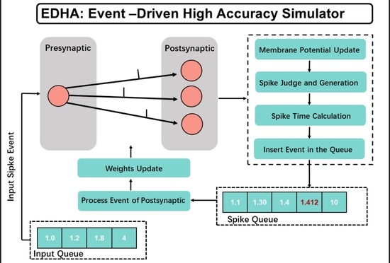
Based on this, this paper will propose a completely event-driven SNN computing simulator named EDHA. By virtue of the event-driven characteristics of the spike neural network, the calculation is carried out when each spike is generated. The calculation complexity is affected by the number of spikes and independent from the time slice. Moreover, even two or more close spikes can be distinguished. EDHA relies on neuron models and synaptic plasticity models to simulate discrete spike events exponentially, and has higher accuracy than clock-driven SNN simulators at the same computational complexity in most cases. The main contribution of this paper lies in (1) an event-driven simulator is proposed for SNN, which reduces the amount of calculation and achieves high speed, and (2) the SNN event-driven simulator has high time accuracy, without increasing computational complexity.

2. Related Works

The following is a detailed description of the current popular SNN simulators, as shown in the

Table 1. Comparison of spiking neural network simulators.

Simulator	Open Source	Simulation	GPU	Programming Language
Brian2 [17]	Yes	clock-driven	Yes	C++ with Python wrapper
Bindsnet [25]	Yes	clock-driven	Yes	C++ with Python wrapper
PyNest [20]	Yes	clock-driven	Yes	C++ with Python interface
Nengo [26]	Yes	clock-driven	Yes	C++ with Python wrapper
NEURON [27]	Yes	clock-driven	No	C++ with Python interface
CARLsim [28]	Yes	clock-driven	Yes	C/C++ with Python wrapper
EDHA (ours)	Yes	event-driven	No	Java

. According to the simulation type, SNN simulators can be divided into clock-driven and event-driven. At present, the method adopted by the SNN simulators is mainly clock-driven, which means each calculation update is measured in time slices rather than spike events. In other words, those clock-driven simulators divide the time into time slices by sampling the time and realize the discretization of the time to accomplish the calculation. As the state of the SNN in a time slice is indivisible and atomic, that is, the SNN in a time slice has only one state, the time slice is the minimum resolution of the SNN. Therefore, the length of the time slice will affect the calculation results [16,17,18,19,20,21]. On the other hand, there are some researchers working on event-driven of spiking neural network [22,23]. The earliest event-driven simulator was proposed that can input parameters to simulate the state of the neuron [23]. After then, an event-driven simulation of a recurrent neural network was proposed to verify the effects of synaptic learning on neuron activity by using the event driven models of IF (integrate-and-fire model), LTP (long-term potentiation), and LTD (long-term depression) [22]. However, their designs are not flexible, unable to define neuron models and learning rules, and not suitable for model training and learning. After that, although the event-driven model of neurons, the event-driven model of synaptic plasticity rules, and other strategies have been proposed for event-driven simulators [24], a complete universal event-driven simulator has not been developed.

Clock-driven simulators currently have some trouble when they are applied to a classification or identification task. First, the time slice size has a great influence on the calculation accuracy and complexity. Figure 1 is a graph of neuron membrane potential attenuation calculated by using the continuous model of the exponential function (ground truth) and the discrete model of the time slice. The continuous curve in the figure can be regarded as the closest to the ground truth. It can be seen from the figure that the length of the time slice directly affects the calculation accuracy, and roughly presents the law of “the shorter the time slice is, the higher the model calculation accuracy is”. However, the shorter the time slice is, the greater the number of iterations are required to calculate the state of the network per unit time, and the amount of calculation will increase accordingly. There is a mutual restriction between the calculation accuracy and the amount of calculation.

Second is the failure of lateral inhibition due to insufficient computational accuracy and resolution. Lateral inhibition [29,30,31,32,33] can prevent multiple neurons from learning the same feature when the same input pattern may trigger multiple postsynaptic neurons during the learning process, which is a key technique in SNN neuron learning. As shown in Figure 2, lateral inhibitory connection occurs when each neuron in the same layer has synaptic connections in which the connection weight is always negative. When there are no lateral inhibitory connections between postsynaptic neurons and each other, postsynaptic neurons fire sequentially in response to presynaptic neuronal spikes. However, when adding lateral inhibitory connection, the earliest firing neuron will inhibit other neurons in the same layer, reduce their membrane potential, and avoid firing. Clock-driven is effective in most cases [12,34]. However, due to the characteristics of the clock-driven method, if two neurons generate spikes in the same time slice, and there is lateral inhibition between the two neurons, then the specific spike sequence of these two neurons is indistinguishable. Due to the wide application of lateral inhibition, this results in the inability to distinguish the specific spike time sequence is unacceptable. In the clock-driven SNN simulator, the processing method is to reduce the length of the time slice [31]. However, this method reduces the probability of two neurons generating spikes in the same time slice, but cannot fundamentally solve this problem.

In order to intuitively statistical the possibility of lateral suppression failure, Equation (1) is used to measure, where $n_r$ is the sum of the number of spikes that fired more than once in a time slice, and n is the sum of the number of spikes. If the time slice is 1ms, and the spike firing time of the output neuron is 1 ms, 1 ms, 2 ms, 3 ms, 3 ms, and 4 ms, then $n_r$ it is 2, n is 6, and $f_r$ is 0.33. Figure 3 shows an example, which is the failure probability of lateral inhibition under different time slices in Brian2. It can be seen from the figure that the results of multiple experiments have certain fluctuations, but the overall follow the positive correlation of “the larger the time slice, the greater the probability of failure of lateral inhibition”. Even if the time slice is 0.01ms, there is still a certain probability of lateral inhibition failure for lateral inhibition, which is about 0.022.

$$f_r=\frac{n_r}{n}$$

(1)

To sum up, most of the mainstream SNN simulators are clock-driven, and there exist the following two problems, which need to be solved. First, there is a conflict between calculation speed and accuracy due to the time slice size. The larger the time slice is, the faster the calculation speed is, and the lower the accuracy is and vice versa. Second, there is a high possibility of lateral inhibition. In the same slice, two or more spikes may be generated, which makes multiple neurons learn repeated features and leads to the failure of lateral inhibition. Therefore, an efficient and high-precision SNN simulator is proposed, which is event-driven to solve the problems.

3. Methods

EDHA is an event-driven simulator. First, the neuron model and synaptic plasticity model should be transformed into event-driven, which is the most important part of SNN. Then, the components of EDHA and the whole process of spike processing will be introduced.

3.1. Event-Driven Model Derivation

In spiking neural networks, the changes of neuron and synaptic models can be divided into unpredictable changes and predictable changes. The former are transient changes in model state caused by pre/postsynaptic spikes which have shorter duration and less computation. The predictable changes refer to the model state changes that change slowly with time during the non-spike period which have longer duration and more computation. In clock-driven simulators, there is no distinction between these two changes [11,35,36]. In clock-driven SNN simulators, the two are not distinguished [16,17,18,19,20,21], but in EDHA, predictable changes caused by pre/postsynaptic spikes can be calculated. Integrals for predictable changes are used which reduces the amount of calculation than time slice iteration. At the same time, because the integration process is not dependent on time slices, but is solved based on analytical solutions, the calculation accuracy depends on the numerical calculation accuracy, thus its calculation accuracy is much greater than that of the clock-driven SNN simulators.

The LIF (Leaky integrate-and-fire model) model is the most widely used neuron model which obtains more accurate neuron characteristics with less computation, and the parameters of LIF model have strong practical significance and the difficulty of parameter adjustment is relatively low. Equations (2) and (3) represent the event-driven model obtained by integrating the standard LIF model. Similarly, as mentioned above, STDP is the most commonly used unsupervised learning method, and Equation (4) is the event-driven model of STDP.

Table 2. Physical significance of parameters.

Parameter	Explanation
$c_0$$c_1$	constant
V	membrane potential
$V_L$	Sodium ion reversal potential
$g_E$	Sodium equivalent conductivity
${\theta }_v$	dimensional constant
${\tau }_v$	leaky time constant of neuron
${\tau }_g$	leaky time constant of conductivity
${\tau }_{+}$${\tau }_{-}$	leaky time constant of STDP
${\sigma }_{+}$${\sigma }_{-}$	renewal magnitude of STDP

shows the physical meanings of the parameters in the equations.

$$V\left(t\right)=c_1{e}^{-\frac{t}{{\tau }_V}}+{\theta }_V\frac{{\tau }_g{\tau }_V}{{\tau }_g-{\tau }_V}{e}^{-c_0}{e}^{-\frac{t}{{\tau }_g}}+V_L$$

(2)

$$g_E\left(t\right)=e^{-\left(\frac{t}{{\tau }_g}+c_0\right)}$$

(3)

$$w=\left\{\begin{array}{cc}{\sigma }_{+}{e}^{-\frac{t_{past}-t_{pre}}{{\tau }_{+}}}\hfill & t_{pre}<t_{post}\hfill \\ {\sigma }_{-}{e}^{-\frac{t_{pre}-t_{past}}{{\tau }_{-}}}\hfill & t_{pre}\ge t_{post}\hfill \end{array}\right.$$

(4)

Figure 4 is an example of neuron membrane potential changes in the event-driven model and clock-driven model. The blue dotted line in the figure is the change of the neuron membrane potential in the clock-driven model. The position where the membrane potential suddenly rises and drops is the moment when the neuron generates spikes in the clock-driven model. The red solid lines are the spike moments of postsynaptic neurons calculated by the event-driven model. The yellow dashed lines are the spike moments of presynaptic neurons. The blue and red numbers in the figure are the exact spike firing time calculated by the clock-driven model and the event-driven model, respectively, at the corresponding time. In the figure, the time slice of the clock-driven model is 1ms, so the minimum resolution of the spike time calculated by the time slice model is 1ms. In contrast, the spike firing time calculated by the event-driven model has much higher accuracy due to its smaller difference to the ground truth, but for display convenience, only one decimal place is reserved. In addition, as the length of the time slice will also affect the calculation accuracy, at a position where the membrane potential rises quickly (near 200 ms in the figure), the spike time calculated by the clock-driven model has a relatively large deviation compared with the result calculated by the event-driven model. Note that the event-driven model in the figure only performs calculations 8 times, and each of them occurs at the position where the presynaptic spike fires, while the clock-driven model performs up to 400 calculations.

From this example, it can be concluded that the event-driven model can obtain higher calculation accuracy with a small number of calculations. Only from the perspective, the event-driven model has achieved obvious advantages. However, due to the practical network of event-driven model is more complex, the specific calculation amount still needs subsequent analysis.

3.2. Structure of EDHA

Figure 5 is a diagram of the module structure of EDHA, and the boxes represent different modules. The green boxes are the those that can be written by the user. Except for the user code at the bottom, the rest of the green boxes are interface modules, and multiple out-of-the-box implementations are provided. The yellow ones represent those modules that cannot be modified. Only a standard implementation is provided, and the function of this part is fixed. The arrow in the figure indicates that there is an interactive relationship between the two modules.

For convenience, bold words represent classes in the code of EDHA in the following part. Soma is used to implement neuron model related functions, and Synapse is used to implement synapse-related functions. Both Soma and Synapse are called by Neuron and do not interact with other modules within the framework. Only mathematical models are needed to be implemented in them, which avoids the overly complex logic of EDHA from affecting the logic of the mathematical model. SNN is the core of EDHA, which realizes the functions of neuron and synapse model calculation, spike transmission, and so on. ReentrantQueue, Logger, and Neuron objects are held internally by SNN. Among them, ReentrantQueue is the interface of spike queue, used to realize neuron spike sorting, spike input, and other functions. Logger is a log interface, used to implement log output, save, and other functions. In addition, EDHA also provides three interfaces: Recorder, Loader, and Channel, which are used to record, load, and transmit network status, respectively. These three interfaces provide simple functional interfaces, which can be called by the user in the user code.

Modules of EDHA are compact, follow the single responsibility principle, splits the module to the greatest extent, and simplifies the user code logic while providing a higher degree of freedom. At the same time, most modules usually only have a direct call relationship with another module, which weakens the dependency relationship between modules and improves the overall flexibility of the framework.

3.3. Neuorn

The Neuron module directly processes the mathematical models of neurons and synapses, and Neuron is an important module. This section introduces the realization of Neuron module and its interaction with other modules.

Neuron is the core of interaction between modules and has a friendly calling relationship with other modules. Neuron calls the Soma module through preSpike (italic words represent methods in the code of EDHA, the same as the rest). It is used to transmit the presynaptic spike to Soma and obtain the next spike firing time predicted by the neuron model. The calling relationship between Neuron and Synapse modules is slightly more. The preSpike method is used to transmit the spike information of the presynaptic neuron to Synapse and obtain the current weight of the synapse for subsequent calculations. The postSpike method is called by the postsynaptic neuron after the postsynaptic neuron fires a spike to notify the Synapse of the postsynaptic spike event to update the weight of the synapse. At the same time, the Neuron can also obtain the weight information of the Synapse through the getWeight method. There is also a call relationship between the Neuron and Neuron, and Neuron can update the state of other Neuron that have synaptic connections with it through the update method. The SNN module calls the Neuron module through the calculate method, so the SNN module does not directly contact the mathematical model of neuron and synapse, and it cannot obtain more information inside Neuron. This can simplify the SNN logic and improve the stability of the code.

3.4. SpikeQueue

SpikeQueue implements ReentrantQueue interface, which is used to realize neuron sorting, and is one of the most important modules of EDHA. EDHA can obtain the neuron that fires the earliest spike from SpikeQueue. At the same time, the spike queue can update the state of the neuron in the queue and ensure that every time a neuron is acquired, the neuron that will fire the earliest spike in the current state can be obtained [37,38]. Based on this, a heap-based SpikeQueue is implemented in EDHA.

The heap has a binary tree structure and can be implemented using pointers. In practical applications, in order to reduce memory usage, array structures are usually used to simulate the heap structure. In addition, the heap structure itself does not make too many requirements for the storage structure. In actual applications, in order to improve memory utilization and simplify calculations, a complete binary tree structure is usually used, that is, all nodes in all layers of the heap are full (have two child nodes) except for the last layer. Nodes stored layer-by-layer in the array.

The use of the minimum heap can achieve most of the requirements of EDHA for SpikeQueue, including neuron insertion, acquisition, and position update. The specific implementation of these parts is no different from the standard minimum heap and is not part of the innovative content of this paper, so this part will not be introduced here. However, the heap structure cannot achieve the deletion of elements, and in SNN calculations, it is often the phenomenon that neurons can emit spikes originally, but then the spikes are inhibited by spikes from inhibitory synapses. At this time, those elements that cannot emit spikes need to be deleted. In order to solve this problem, a small trick is used in EDHA to realize this function. That is, for those elements that need to be deleted, they are not directly deleted but marked, indicating that the element is invalid; invalid elements are skipped when getting elements. This solves the problem that the minimum heap cannot delete elements.

Spike queue update is an important part of event-driven spiking neural network. As shown in Algorithm 1, it is the pseudocode of SpikeQueue update.

Algorithm 1 Pseudocode of SpikeQueue update

Require: InputQueue:initial the input spike queue; SpikeQueue:initial the complete spike queue; $t_{thr}$: the threshold membrane potential; $t_{pre}$:the most recent presynaptic spike time; $t_0$: current time; $t_{last}$: The last predicted time of the postsynaptic spike time, $t_{last}$ > 0 represents will produce postsynaptic spike Ensure: Updated spike queue SpikeQueue 1: while$t_{pre}$do 2:  Calculate the current membrane potential $V_0$ 3:  Predict the current possible maximum spike time $t_{peak}$ and $V_{peak}$ 4:  if ($t_{peak}$ > $t_0$) AND ($V_{peak}$ > $V_{thr}$) then 5:   Calculate the exact spike time $t_{spike}$ 6:   if $t_{last}$ > 0 then 7:    update spike time of current neuron in SpikeQueue 8:   else 9:    Insert current neuron into SpikeQueue 10:     end if 11:     $t_{last}$ = $t_{spike}$ 12:    else 13:     if $t_{last}$ > 0 then 14:      delate current neuron from SpikeQueue 15:     end if 16:     $t_{last}$ = −1 17:    end if 18: end while

Table 3. Comparison of time complexity of spike queue constructed by three data structures.

Data Structure	Insert	Update	Deletee	Get
Minimum heap	O(log(n))	O(log(n))	O(1)	O(1)
Array	O(n)	O(n)	O(n)	O(1)
Linked list	O(n)	O(n)	O(1)	O(1)

shows the comparison of time complexity of spike queue constructed by three data structures. When the number of neurons is large, the spike queue based on minimum heap has obvious advantages in speed.

3.5. Workflow of EDHA

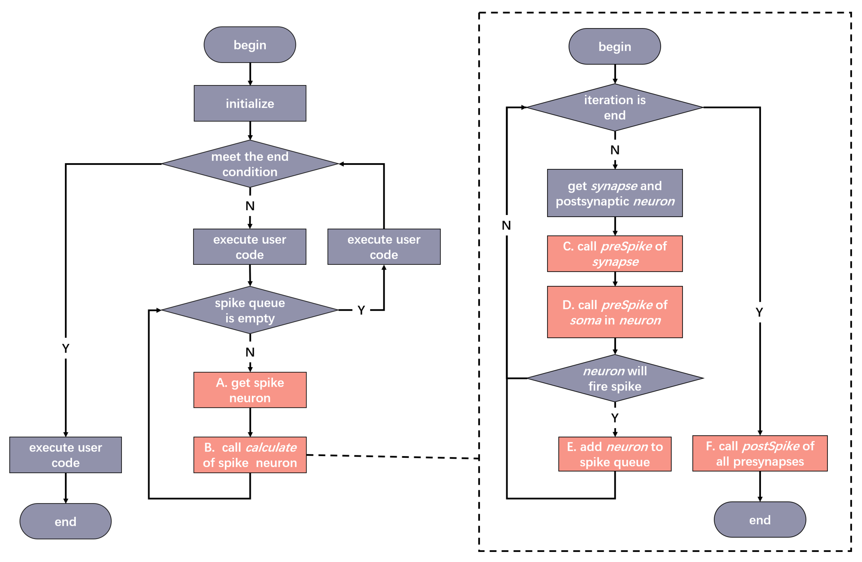
Figure 6 is the workflow of EDHA, the left is the overall workflow, and the right is the details after step B is expanded. The steps in red in the flowchart correspond one-to-one with the steps marked with letters in Figure 7, indicating the calling relationship between the modules. The calling sequence of EDHA is as follows:

(1)

Initialize the network state, including the creation of neurons, the connection of neurons, and the creation of SNN objects.

(2)

Determine whether the end condition set by the user is met, if it is met, go to step (9); otherwise, go to step (3)

(3)

Enter the loop, execute the user code, including spike loading, resetting the state of the object, etc.

(4)

Determine whether there are neurons in the spike queue. If there are no neurons, go to step (8); otherwise, go to step (5).

(5)

Obtain spike neuron, as shown in Figure 1, Figure 2, Figure 3, Figure 4, Figure 5, Figure 6, Figure 7, Figure 8, Figure 9 and Figure 10. This step is obtained by SNN calling ComboQueue. ComboQueue will compare the neurons in SpikeQueue and InputQueue and select the one that emits the spike earlier.

(6)

Call the calculation method of the spike neuron. This step is implemented by SNN calling Neuorn, and enter the flowchart on the right.

(6.1)

Determine whether the postsynaptic neuron traversal of the current neuron is completed, if the traversal is completed, go to step (6.7); otherwise, go to step (6.2).

(6.2)

Obtain the postsynaptic neuron (bold together with italic word represent variates) and the corresponding synapse.

(6.3)

Call synapse’s preSpike method to obtain synaptic strength information and notify the synapse of presynaptic spike.

(6.4)

Call Soma’s preSpike method in neuron to update Soma’s internal state.

(6.5)

Determine whether the neuron fires a spike, if no spike is fired, go to step (6.1), otherwise go to step (6.6).

(6.6)

Add neuron to the spike queue and go to step (6.1).

(6.7)

Call the postSpike method of all pre-synapses (that is, the synapses that use the current neuron as the postsynaptic neuron). Notify the synapse that a postsynaptic neuron spike event has happened.

(6.8)

Go to step (7).

(7)

Go to step (4).

(8)

Execute user code, including status records after a single calculation is completed, data transmission, etc.

Figure 7 shows the calling relationship of the EDHA core modules (EDHA code is available at http://www.snnhub.com/EDHA/code (access on 12 August 2021)). From top to bottom, the containing relationship between the modules is shown. The upper module is contained in the lower module. The arrows indicate the calling relationship that the caller points to the callee. The letter labels on the arrows correspond to the labels in Figure 6, and multiple identical labels indicate that they are completed in the same step in Figure 6.

4. Experiments and Results

In order to illustrate the computational speed and accuracy advantages of EDHA, this section will demonstrate these factors through experiments. Several current mainstream SNN simulators mentioned above are compared including Brian2 [17], Bindsnet [25], PyNest [20], Nengo [26], NEURON [27], CARLsim [28], and Brian2GeNN [39], among which Brian2 is clock-driven framework with the largest number of users and the most active community. Bindsnet benefits from the flexibility and command execution of PyTorch and the simulation speed is relatively fast [25]. Nengo calculates a population of neurons, which is normally used to simulate the brain or large scale neural networks [27]. NEURON is flexible but not easy to be used for the benchmarked network structure and the speed is not competitive either. From previous comparative experiments [25], the simulation speed of PyNest is slower than Bindsnet. Because EDHA only supports CPU platform at present, it can not be compared with GPU simulation platforms, such as CARLsim and Brian2GeNN. Therefore, the following will mainly select Brian2 and Bindsnet for comparison. The calculation accuracy and calculation speed will be analyzed and compared respectively.

4.1. Accuracy Comparison

In the calculation of SNN, the accuracy is mainly reflected in two parts: the accuracy of the spike firing time and the resolution of the spike firing time. The accuracy of the spike time refers to the difference between the calculated spike time and the true spike time [40,41]. The greater the difference is, the lower the accuracy of the spike time is. Spike time resolution refers to the shortest time unit that can distinguish spikes in the calculation result. As both Brian2 and Bindsnet are clock-driven frameworks and will have similar results in spike time accuracy, only Brian2 is discussed here. This section will analyze the calculation accuracy of EDHA from these two aspects compared with Brian2. The first analysis is the accuracy of the spike time. In order to analysis this, the truth value is required. The Brain2 simulation results with a time slice length of 0.0001 ms that is used as the true value because the true value cannot be obtained directly. One thing that has to be explained is that there is no way to know which of the calculation results of EDHA or Brian2 at a simulation step of 0.0001 ms is more accurate. However, it is certain that the shorter the simulation step, the higher the calculation accuracy [42,43]. Therefore, the relatively extreme value of 0.0001 ms is selected as the comparison standard. Figure 8 shows the spike accuracy changes under different time slices in Brian2. The accuracy is measured by the Euclidean distance between the calculated spike time vector and the true spike time vector. The closer the distance is, the higher the similarity of the spike time is. The calculation formula of the spike time vector distance is as Equation (5).

$$d=\sqrt{\sum _{i=1}^N{\left(a_i-b_i\right)}^2}$$

(5)

Among them, N is the number of spikes in the spike time vector, $a_i$ is the firing time of the i-th spike of the target spike vector, and $b_i$ is the firing time of the i-th spike of the actual spike vector.

The green dash-dotted horizontal line in the figure is the Euclidean distance between the spike time vector calculated by EDHA and the true spike time vector. The subgraphs embedded in the figure are the local details when the time slices are 0.01 and 0.02 ms. The dotted line near time slice of 0.9 ms in the figure indicates that the number of spikes generated at this position is not equal to the number of true spikes, so Equation (5) cannot be used for calculation. It can be seen from the curve of Brian2 that as the time slice gradually increases, the difference between the spike time and the true value becomes larger and larger, and the spike time accuracy becomes increasingly worse even when it lacks spikes. These phenomena seriously affect the calculation accuracy. In other words, when the time slice is a small value of 0.01 ms, the spike time accuracy still has a certain gap compared with the result calculated by EDHA. It is brought by a time slice as small as 0.01 ms whose amount of calculation consumed is unacceptable. In contrast, EDHA has a significant advantage in spike time accuracy.

Figure 8. The comparison of spike time accuracy between Brian2 and EDHA.

Figure 8. The comparison of spike time accuracy between Brian2 and EDHA.

In contrast, EDHA, because its time resolution in principle is a computer numerical resolution, the probability of lateral inhibition failure is always zero. From the perspective of lateral inhibition, EDHA has significant advantages over Brian2 and other SNN simulators based on clock-driven methods.

4.2. Speed Comparison

As introduced before, EDHA saves the calculation process of a large number of predictable parts in the clock-driven model and only retains the calculation process of the unpredictable part. EDHA only performs calculations when spikes are generated in the SNNs. The frequency of calculations is significantly lower than that of the clock-driven model. However, the single calculation amount of EDHA is much higher than that of the clock-driven model, and it also involves more complex calculation processes such as exponential and logarithmic. The calculation amount of a single spike is difficult to compare with Brian2. As the calculation amount of EDHA depends on the number of spikes, the calculation amount of clock-driven simulators such as Brian2 and Bindsnet depends on the calculation time and the time slice length, so in order to compare the performance of the two more fairly. This section selects an MNIST recognition network based on unsupervised learning that is widely used in SNNs for comparison. Because it is closer to the actual use scenario, it can show the calculation speed of the two simulators more comprehensively and fairly.

The network used in this experiment is derived from Diehl’s paper [31] whose structure is shown in Figure 9. It is used to realize the unsupervised MNIST recognition task. The network has a two-layer structure, where the input layer is 28 × 28, which is the same as the input picture structure, and the output layer is 20 × 20 together with lateral inhibition. Detailed attributes used in the network are shown in

Table 4. Attributes that were used in the speed comparison network. EDHA with asterisk is the EDHA run on the optimized model.

Attribute	Brian2	Bindsnet	EDHA	EDHA *
Input layer size	28 × 28	28 × 28	28 × 28	28 × 28
Output layer size	20 × 20	20 × 20	20 × 20	20 × 20
Inhibited layer size	20 × 20	20 × 20	0 1	0 1
Number of smaples in training set	60,000	60,000	60,000	60,000
Number of samples in testing set	10,000	10,000	10,000	10,000
Averaged number of spikes per sample	2284.38	2284.38	2284.38	136.54
Training Epoch	3	3	3	4

No inhibited layer is required to implement lateral inhibition in EDHA.

. Note that EDHA* is EDHA run on the optimized model. In this paper, time coding is adopted to reduce the number of spikes per sample in EDHA*, while EDHA means using the same frequency coding as Diehl’s. The experimental platform of this experiment is Intel i5-6500 CPU, 16 GB memory.

Figure 9. Network structure of Deihl’s work [31].

Figure 9. Network structure of Deihl’s work [31].

Table 5. Time required for EDHA and Brian2 to run on the MNIST unsupervised model. EDHA with asterisk is that EDHA ran the optimized model.

Simulator	CPU	RAM	OS	Accuracy
Brian2	Intel i5-6500 (3.2 GHz × 4)	16G	win10	87.7%
Bindsnet	Intel i5-6500 (3.2 GHz × 4)	16G	win10	86.7%
EDHA	Intel i5-6500 (3.2 GHz × 4)	16G	win10	87.9%
EDHA *	Intel i5-6500 (3.2 GHz × 4)	16G	win10	88.0%
EDHA *	Apple M1(3.2 GHz × 8)	8G	BigSur	87.9%
EDHA *	AMD Ryzen 5 2500U (3.6 GHz × 4)	6.3G	win10	88.0%

and Figure 10 show the running time of unsupervised MNIST recognition network. The training and evaluating time of Brian2 and Bindsnet are 228.33 h and 18 h, and 1094.1 h and 18.0 h, respectively. In contrast, the network also based on frequency coding which was taken in Diehl’s work [31] takes 17.3 h and 3.93 h to train and evaluate, respectively, on EDHA. The speed is dramatically increased. At the same time, the network accuracy calculated by EDHA is not significantly different from Brian2 and Bindsnet. In addition, according to the characteristics of EDHA, the model coding method is optimized to reduce the number of spikes, which can greatly improve the calculation speed of EDHA on the model, and it hardly affects the performance of the model. Note that because the CPU used has 4 cores, Brian2 has a multi-threaded acceleration, so it will occupy all 4 CPUs, and EDHA is based on single-threaded implementation, so only one of the cores is used and the computing resources used is much less than Brian2. In the case of Bindsnet, it makes full use of pytorch, which is flexible and simple to operate, but is heavily hardware-dependent. Like Brian2, Bindsnet is also multi-cpu, but its simulation speed is always lower than that of Brian2 on the same experimental platform. By the way, the time slice length used by clock-driven framework in the calculation is 0.1 ms. As the result of the previous analysis, if want to obtain similar calculation accuracy, they need to use a time slice at least 0.01 ms, and the required time is about 10 times the current experimental result which means that more advantages will be taken by EDHA in calculation speed if the model has a higher requirement in spike time resolution. In summary, this experiment shows that EDHA has obvious advantages over Brian2 in terms of calculation speed. Last but not least, thanks to the cross-platform characteristics of Java, EDHA can run well on Macbook air with M1 CPU and Big Sur OS or platforms with other CPUs.

Figure 10. Time spent by models in Table 5. For convenience of display, height of bars are calculated by $h=lo{g}_{10}\left(time\right)$.

Figure 10. Time spent by models in Table 5. For convenience of display, height of bars are calculated by $h=lo{g}_{10}\left(time\right)$.

4.3. Benchmarking

In order to compare the above competitive SNN simulation frameworks, a simulation network will be designed to benchmark. The network is two-layer which each layer consists of n neurons. In detail, the input layer is n Poisson input of which the firing rate is preseted, and the output layer is output according to the framework’s LIF model and STDP learning rules. The two layers are all-to-all connected, and the connection weights are fixed and learnable, respectively. In the simulation, n is varied from 100 to 3000 in steps of 100, and run each simulation with every library for 1000ms, with a time resolution of Brian2 and Bindsnet dt = 1.0 ms. The experimental platform of this simulation is Intel i5-6500 CPU, 16 GB memory.

Figure 11 shows the simulation results with fixed connection weight (0, 1) distribution. Each subgraph represents the simulation with the preset spike firing rate of neurons in the input layer. Considering that the wave frequency of human brain under normal activity is about 5–10 Hz, the simulation is conducted at 0.1 Hz, 0.5 Hz, 1 Hz, 2 Hz, 5 Hz, and 10 Hz, respectively. As can be seen from Figure 11, the actual simulation time of clock-driven Brian2 and Bindsnet differs little at different spike firing rate, while the simulation time of event-driven EDHA is closely related to the number of spikes. The curve of Brian2 is always stable, and the simulation time is always less than that of Bindsnet. From the first four subgraphs, at n < 2000 and spike firing rate < 1 Hz, EDHA is the fastest, and even at 2 Hz was comparable to the Bindsnet. In general, EDHA is competitive in the case of small and medium-sized networks and sparse input spikes.

Figure 12 shows the simulation results of the connection of learnable weights, in which the learning rules of weights are all STDP rules of the corresponding framework. As can be seen from the figure, EDHA is the fastest at n < 3000, spike firing rat e < 10 Hz. Brian2 is the slowest because of the plasticity is clock-driven, and the simulation time increases exponentially with the increase of network size. Bindsnet, by contrast, is somewhere in the middle. To sum up, the framework mentioned above is simulated for different network sizes and different spike firing rate of fixed weight connections and learnable weight connections. The comprehensive results show that EDHA benefits from the event-driven characteristics and has great advantages in simulation speed and simulation time in the case of small and medium-sized networks with sparse input.

5. Discussions

An event-driven simulator is presented which has significant advantages over the traditional clock-driven SNN simulators in terms of accuracy and speed. The following sections discuss EDHA’s improvements and future works.

5.1. Comparison with Prior-Art

Compared to the previous event-driven simulator [22], EDHA has the following three improvements: First, EDHA is more flexible, and the neuron and synaptic model, spike coding, and simulation time can be customized. Second, EDHA can implement the LIF model, which is more consistent with real biological neurons, while the event-driven simulation used IF model. Third, EDHA has higher time accuracy and is more beneficial to STDP learning and lateral inhibition, which is conducive to SNN learning.

5.2. Model Compatibility

From the previous introduction to the principle of event-driven models, it can be known that the event-driven model is mainly realized by integrating the part of the model that decays over time to avoid the loss caused by repeated calculation of these parts. Therefore, EDHA requires that the neuron and synapse model can be integrated [37,44,45] or the method of solving the integral numerical solution is used instead of the analytical solution of the integral. However, the use of numerical solutions will largely lead to the disappearance of EDHA’s advantages. Especially when using a numerical solution instead of an analytical solution for a neuron model, the problem of lateral inhibition failure is prone to occur. However, the difference with the clock-driven model is that in the process of solving the numerical solution, the integration step length is not fixed, and the integration step length can be adjusted according to the needs. A longer step length is used where the accuracy requirement is lower, and vice versa. A shorter step length is used to improve the overall calculation accuracy. Therefore, there is a balance between the amount of calculation and the calculation accuracy. The current version of EDHA does not provide relevant code implementation for this part of the content, which is also the future development direction of EDHA.

5.3. Multi-Threading Acceleration

As mentioned earlier, EDHA does not currently use any acceleration technology, and all calculations are done on a single thread. Although the current single-threaded EDHA has been able to achieve good calculation accuracy and speed, if proper acceleration technology can be used, the calculation speed of EDHA can undoubtedly be brought to a higher level. This point was fully considered at the beginning of the EDHA design. It can be seen from Figure 6 and Figure 7 that the calculation process in EDHA mainly occurs in the calculate method of the Neuron module, and in the calculating process, all postsynaptic neurons and their corresponding synapses of the current neuron will be traversed. Each postsynaptic neuron and synapse only performs calculation once within one calculate calling, and there is no sharing of variables between each other, so it is very suitable for distributing to multiple threads for calculation. By packaging the computing tasks of synapses and postsynaptic neurons into individual computing tasks, and then using multi-threaded pooling technology, multiple computing threads continuously acquire computing tasks to complete the computing process.

5.4. Large-Scale Simulation

At present, EDHA has a good calculation speed. However, compared to the scale of the human brain (100 billion [46]), the scale of neuron calculations that EDHA can complete is still too small. In order to perform calculations and simulations on a larger scale, or even reach the scale of the human brain, a single calculation is powerless, and more computers are needed to join the simulation. When performing large-scale simulations, a computer can be regarded as a brain area [47] of the brain to perform specific functions. Networks are used for communication between computers. EDHA now provides standardized spike input and output interfaces, and by means of connecting these interfaces to the network, the purpose of collaborative computing by multiple computers can be realized and larger-scale neuron simulation calculations can be completed.

6. Conclusions

This paper proposes a SNN simulator called EDHA, which utilizes the SNN event-driven characteristics, and the models of neuron and synapse are all event-driven. EDHA solves the conflict between the calculation speed and accuracy of the clock-driven SNN simulators, and the lateral inhibition failure caused by the existence of time slice. In addition, it reduces a large number of calculations and realizes high computational accuracy when the spike frequency is not too high and the layer-to-layer connection is not too large, especially suitable for sparse input spikes and sparse connections, which is also the most common situation of brain work. In the future, we will develop parallel computing modes of multi-core parallel computing and distributed parallel computing.