A Low-Cost Hardware-Friendly Spiking Neural Network Based on Binary MRAM Synapses, Accelerated Using In-Memory Computing

Abstract

In recent years, the scaling down that Moore’s Law relies on has been gradually slowing down, and the traditional von Neumann architecture has been limiting the improvement of computing power. Thus, neuromorphic in-memory computing hardware has been proposed and is becoming a promising alternative. However, there is still a long way to make it possible, and one of the problems is to provide an efficient, reliable, and achievable neural network for hardware implementation. In this paper, we proposed a two-layer fully connected spiking neural network based on binary MRAM (Magneto-resistive Random Access Memory) synapses with low hardware cost. First, the network used an array of multiple binary MRAM cells to store multi-bit fixed-point weight values. This helps to simplify the read/write circuit. Second, we used different kinds of spike encoders that ensure the sparsity of input spikes, to reduce the complexity of peripheral circuits, such as sense amplifiers. Third, we designed a single-step learning rule, which fit well with the fixed-point binary weights. Fourth, we replaced the traditional exponential Leak-Integrate-Fire (LIF) neuron model to avoid the massive cost of exponential circuits. The simulation results showed that, compared to other similar works, our SNN with 1184 neurons and 313,600 synapses achieved an accuracy of up to 90.6% in the MNIST recognition task with full-resolution (28 × 28) and full-bit-depth (8-bit) images. In the case of low-resolution (16 × 16) and black-white (1-bit) images, the smaller version of our network with 384 neurons and 32,768 synapses still maintained an accuracy of about 77%, extending its application to ultra-low-cost situations. Both versions need less than 30,000 samples to reach convergence, which is a >50% reduction compared to other similar networks. As for robustness, it is immune to the fluctuation of MRAM cell resistance.

1. Introduction

With the development of artificial intelligence in recent years, the third-generation artificial neural network (Spiking Neural Networks, SNNs) driven by spike events is gradually becoming a research hotspot. Compared with traditional artificial neural networks, the SNN has the advantages of higher computational efficiency and stronger biological rationality. Attempts to implement hardware-accelerated spiking neural networks have been made by academia and industry, such as IBM TrueNorth [1] and Intel Loihi [2]. The TrueNorth chip includes 1 million neurons and 256 million synapses within 430 mm² under a 28 nm process. It features event-driven, hybrid clock, near-memory computing, and other technologies, consuming 65 mW of power typically. Loihi uses an on-chip network for communication, whose neural cores are time-division-multiplexed to simulate each part of the neuron. The whole chip implements 128 neuromorphic cores on a single chip of 60 mm². These two chips, as a representative of the traditional CMOS implementation of a spiking neural network, have common problems: they simulate the mechanism of the brain only at the algorithm level, instead of using more efficient and biologically reasonable methods, which has caused a high complexity and high cost of hardware design, and has limited the processing power because of the inherent bottleneck of Von Neumann architecture [3].

Due to the shortcomings of the digital CMOS logic implementation described above, the memristor-based SNN has been proposed as an alternative. Methods to implement basic logic gates using memristive devices have been proposed [4,5]; however, due to the extra operation circuits and lower integration density, it is impossible to replace the traditional large-scale CMOS logic circuits in neural network applications that require extremely high computing power. Subsequently, memristors were applied as synapses to accelerate the SNN more efficiently. This is closer to how the brain actually works, leading to improved performance, enhanced energy efficiency, and smaller area [6,7].

Although the memristor-based synapse is believed to simulate the brain more efficiently and reasonably, the SNN based on it still needs appropriate algorithms to outperform the traditional ANN. There is an inevitable question with the SNN training algorithm, that the spike train cannot be differentiated as with the floating-point number in artificial neural networks. Therefore, it was not possible for mainstream learning methods, such as back-propagation [8], to be directly ported to SNNs. As a result, a variety of artificial alternative methods that imitate back-propagation in the form of spikes were proposed in [9,10,11]. These methods have worked adequately to a certain degree but have resulted in a lot of additional statistical calculations. Moreover, in [12,13,14,15,16], the ways of converting ANN to SNN were studied, but the biological plausibility of such methods has not been confirmed.

In order to achieve better training, unsupervised SNN training based on spike-timing-dependent plasticity (STDP) has been proposed. Diehl et al. [17] proposed a spiking neural network that used STDP learning rules with lateral inhibition and a LIF dynamic model. It consisted of 6400 neurons and achieved a 95% accuracy after being trained with 200,000 training samples. The SNNs in [18,19] were also based on STDP, but their learning rules were temporally adjusted to enhance robustness. The disadvantage of these STDP-based networks is that they require the memristor synapses to have continuous tunability and high reliability, which is difficult for current technology to produce on a large scale.

Considering the manufacturability of the memristor synaptic array, research of the spiking neural network based on the binary memristor has been performed. Zhao et al. proposed a method for two-bit multi-state MRAM cells for weight storage [20,21]. However, this method calls for complicated peripheral circuits: more sense amplifiers, which take a lot more area; and special operating modes, which take two steps to write new weight values. In addition, these devices are still not as reliable as single-level MRAM cells. Zhou et al. tried to dispose of several neural behaviors, such as leakage currents, refractory periods, lateral inhibition, and adaptive threshold voltages, to simplify the SNN hardware architecture [22], but failed to reduce the number of synapses of the array, because a large number of neurons are still required to reach decent accuracy.

This paper proposed a low-cost hardware-friendly SNN based on binary MRAM synapses. The synaptic array consisted of binary MRAM cells capable of in-memory computing. The input spike trains of the array were designed to be sparse enough so that the design of peripheral circuits such as the sense amplifier (SA) can be simplified. We also proposed a new learning rule where adds and subtracts to the 8-bit discrete weights are performed by a single step. Finally, to further reduce the hardware complexity, we created a constant-leaking LIF dynamic neuron model, which does not need the digital circuits to carry out difficult exponential operations. The simulation results on the MNIST dataset showed that our network could achieve an accuracy of up to 90.6% with 1184 neurons and 313,600 synapses in total. On the other hand, if the source images are 16 × 16 low-resolution, our smaller network with 384 neurons and 32,768 synapses still maintains an accuracy of 77.0%. As for convergence, the network requires only about 30,000 samples of the MNIST dataset to reach a stable accuracy, which is less than most other works. In addition, this network is resistance-fluctuation-proof, so it works well with nonideal MRAM cells, as shown in the latter results.

The main contributions and innovations of this paper are:

• We proposed a low-cost hardware-friendly spiking neuron network architecture with a small number of neurons and synapses. It is based on binary MRAM devices and can be accelerated using in-memory computing to implement high-efficiency neuromorphic computation.
• We introduced a discretized learning rule to train the network. It is specially optimized for fixed-point weights, which lowers the hardware complexity, but is still able to reach convergence within much fewer samples than other works can.
• We tested our network and learning rule on the MNIST dataset, and the result showed that the recognizing accuracy is decent enough compared to other similar works, and it has great robustness against MRAM’s technology problems. It even works well in ultra-low-cost situations.

2. High Accuracy, Low Sample Size, Hardware-Friendly SNN Based on MTJ Synapses

2.1. SNN Architecture

The spiking neural network in this article is two-layer fully-connected. It features an input layer of encoders, converting the pixels into spike trains, and a feature layer of which the neurons are trained to respond to different digit patterns. These responses are defined by the weights of synapses, which are stored in the binary MRAM synaptic array. Each MRAM cell in this array contains an MTJ (magnetic tunnel junction), and each MTJ’s resistance is used to store one bit of a synaptic weight. The spikes generated by encoders are sent to the crossbar array, which acts as the connections between two layers, and accelerates the computing process of the post-synaptic neurons. Results after the analog multiply-add are sensed and then processed by the post-processing circuit, including simulating the dynamic behavior and identifying the spikes generated by post-neurons. Finally, for training, synaptic weights are updated according to our single-step STDP learning rule; for testing, winner-take-all was performed to decide which digit the input is.

Compared to similar work, we have greatly reduced the number of neurons, which leads to a reduction in the number of rows, thus meeting actual manufacturing capability. Our encoders are designed multi-mode to provide flexibility for different situations, and the number of encoders can be changed to adapt to images in different resolutions. The standard exponential STDP rule used in the SNN learning process has also been modified to fit low-precision fixed-point weights. Finally, we use a new dynamic model for feature layer neurons to reduce the complexity of circuit implementation. The overall block diagram of the architecture is shown in Figure 1.

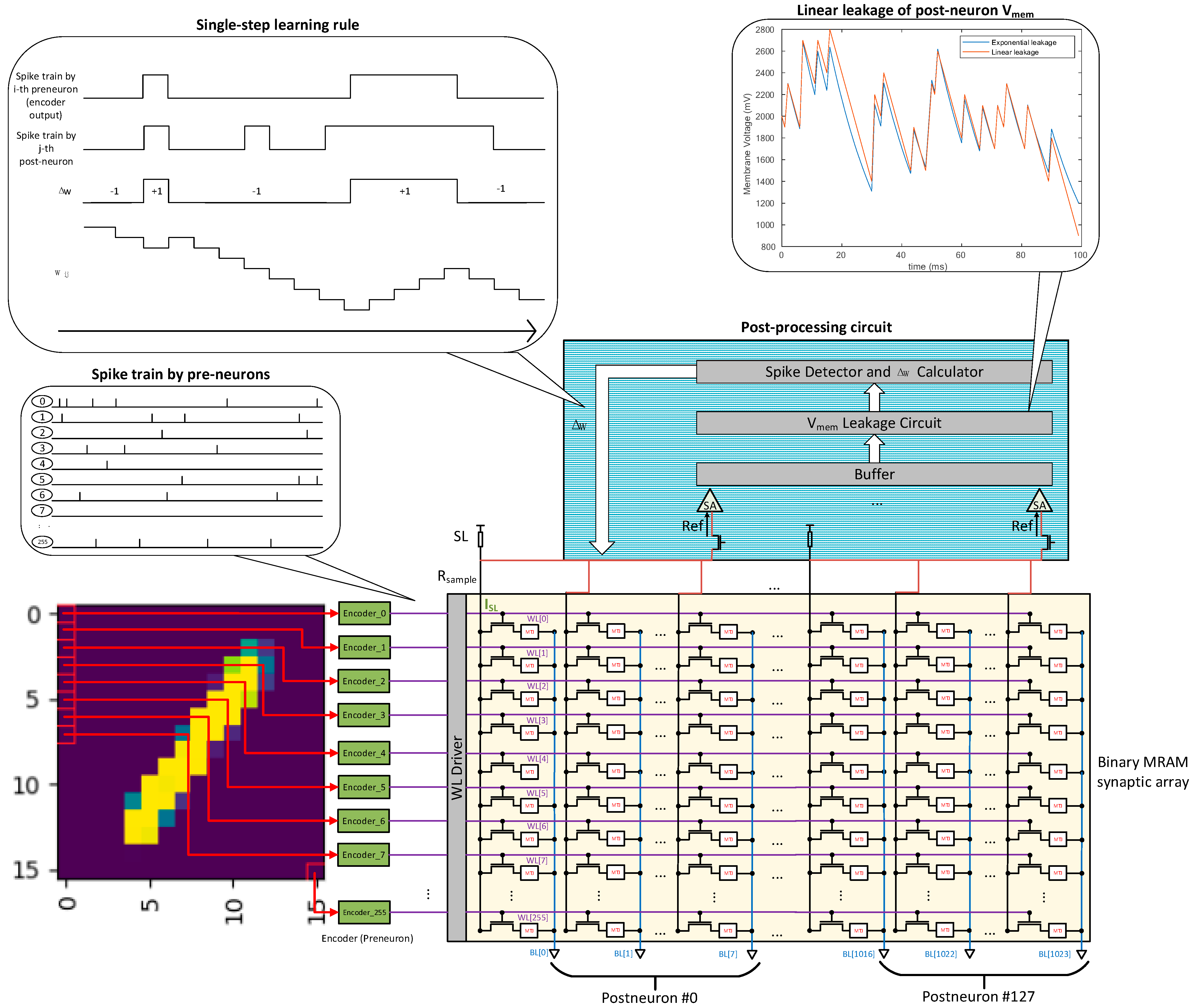
2.1.1. Binary MRAM-Based Synaptic Array

The neural network simulates synaptic plasticity by updating the weights of the synapses. Previous work has shown that 8-bit floating-point weights for ANN training are good enough to achieve decent results [23]. This work is based on a similar idea and uses 8-bit fixed-point numbers to store the weights of the synapses.

The research of Zhang and Zhao et al. [20,24] showed that multi-level cell (MLC) MRAMs still need to overcome reliability problems. As a solution, specially optimized cell structure and read–write methods were designed, which increases the cost and difficulty of application. Given this, we chose to build our network on a single-level MRAM cell, and combine eight 1-bit MTJ to represent an 8-bit weight value. Doing so maintains compatibility with traditional memory manufacturing processes while ensuring the correctness of the calculation results:

Taking the case of the 256 input layer neurons as an example, the 8-bit weight value connecting the i-th input layer neuron and the j-th feature layer neuron is:

$$w_{ij}={\displaystyle \sum }_{k=0}^7{2}^k·w_{ij}\left[k\right]$$

(1)

where w_ij[k] is the k-th bit of w_ij, so the result Y of multiplying the input X and the weight w is:

$$Y_j={\displaystyle \sum }_{i=0}^{255}{X}_i·w_{ij}={\displaystyle \sum }_{i=0}^{255}{X}_i·{\displaystyle \sum }_{k=0}^7{2}^k·w_{ij}\left[k\right]$$

(2)

According to Kirchhoff’s law, the relationship between the current I_k on each bitline and the input X_i and MTJ conductance G_k is:

$$I_k={\displaystyle \sum }_{i=0}^{255}{X}_i·G_k$$

(3)

The current on the 8 bitlines corresponding to the same feature neuron is sensed by SA, and shift-added, which gives:

$${\displaystyle \sum }_{k=0}^7{2}^k·f\left(I_k\right)={\displaystyle \sum }_{k=0}^7{2}^k·{\displaystyle \sum }_{i=0}^{255}{X}_i·w_{ij}\left[k\right]$$

(4)

Equation (4) is actually equal to Equation (2). Therefore, the sum of the input currents of the neuron can be obtained by simply adding the column currents of 8 different columns representing the same weight through sensing, quantization, and shifting.

2.1.2. Multi-Mode Input Encoder with Spike Sparsity

Each pixel of the input image corresponds to an input layer neuron (spike encoder). The input layer neuron transforms the grayscale value of the pixel into a spike train. Many schemes for encoding could be applied, mainly divided into rate coding and temporal coding. Our network supports three different rate-coding methods: 1-bit fixed frequency encoding, 8-bit variable frequency encoding, and Poisson encoding. In 1-bit fixed frequency coding, the bit depth of the input picture is 1-bit, that is, black and white images. For each pixel, if the pixel value is ‘1’, a spike train with a fixed frequency and a fixed time interval is generated; if the pixel value is ‘0’, no pulse is generated. This method reduces the amount of input data at the expense of a small accuracy loss, and helps to improve energy efficiency and anti-interference ability.

In 8-bit variable frequency coding, a spike train whose frequency is proportional to the pixel grayscale value will be generated. The pixels of the input picture are 8-bit grayscale values. The larger the pixel grayscale value is, the more frequently the input neuron fires.

In Poisson coding, a spike train conforming to the Poisson distribution, with its average firing frequency proportional to the pixel grayscale value, will be generated. The maximum value of the average firing frequency of the input layer neurons is set to 156.25 Hz (when the pixel grayscale value is 255). The pulse width is 25 ms, and the amplitude is 1 V. These time parameters are carefully chosen to avoid the complex multiplication operations when using digital circuits to implement. Instead, only shift operations are needed. Our network also supports the MNIST dataset in resolutions as low as 16 × 16, which is critical to the feasibility of the circuit, because the higher-resolution SNN will require MRAM arrays with more rows, making it difficult for the memory to work correctly.

We captured some of the output spike trains from input layer encoders, as shown in Figure 2. It can be seen that, due to the sparseness of spike output, less complicated SA arrays could work adequately for further processing, because there will almost never be too many neurons firing at the same time. As for the other coding schemes, this conclusion is also supported by the statistics of simulation results, which gives the probability distribution of numbers of input neurons that fire at the same time under different resolutions, as shown in Figure 3. As the timing of firing can be controlled (instead of being random in Poisson coding), the sparseness of the spike trains can be guaranteed as well. As a result, the area and power of the SA array can be significantly reduced, causing a much smaller cost of the peripheral circuit.

2.1.3. Learning Rule with Single-Step Fixed-Point Weight Update

In the ANN, calculations involved in training include multiplication, addition, and derivation. In order to accelerate these complex operations, various application-specific integrated circuits (ASICs) have been proposed, such as Google TPU [25] and NVIDIA CUDA GPU [26]. These implementations have been widely used because of their high performance, but there is a general problem of energy efficiency in these massive digital circuits. In spiking neural networks, spike-timing-dependent plasticity (STDP) is usually used as an efficient learning rule because it is similar to brain activities [17]. The STDP learning rule defines that the weight update Δw is exponentially related to the fire time of the pre- and post-neurons. However, this exponential relation makes digital implementation very expensive. Thus, to make the training method more hardware-friendly, we proposed a simplified STDP learning rule for weight updating:

$$\mathsf{\Delta }w=\{\begin{array}{c}+1 level, if v_{pre}=1 V when post-neuron fires\\ -1 level, if v_{pre}=0 V when post-neuron fires\end{array}$$

(5)

where v_pre is the voltage of the pre-neuron. As v_pre is either 0 or 1 V (corresponding to the pre-neuron firing or not firing), Δw can be calculated by performing bitwise AND of the input neuron state and the feature neuron state. This greatly simplifies the computational complexity, and the action of updating collaborates well with our fixed-point weights.

2.1.4. Feature Layer Neuron Model with Linear Leakage

The feature layer neurons receive spikes from the input layer neurons through synapses, and their membrane voltage u(t) changes according to certain rules. This work uses the LIF model, and its dynamic behavior is as follows:

$${\tau }_m\frac{du\left(t\right)}{dt}=-\left[u\left(t\right)-u_{rest}\right]+R\cdot I\left(t\right)$$

(6)

where u_rest is the resting potential, R is the resistance, and I is the sum of the currents. When current I(t) = 0, u(t) decays exponentially, with the time constant τ_m being 100 ms. The exponential decay behavior of the membrane voltage in the LIF model can be implemented using analog circuits, but additional high-precision ADCs will be needed for subsequent processing; digital circuits can also be used to simulate the exponential decay, but complexity and cost will be greatly increased. Therefore, we designed a neuron model with linear leakage at a fixed leakage rate—the membrane potential always decreases by 4 V (which equals the threshold voltage) within 350 ms (which is the time window length of a picture).

There is lateral inhibition between neurons in the feature layer. We define lateral inhibition as, once a certain feature layer neuron fires, all feature layer neurons are reset to the initial potential in the next time step and the refractory period is maintained.

2.2. SNN Workflow

As shown in Figure 4, The circuit-level workflow of our spiking neural network contains three tasks: training, pre-classification, and classification. The training task dynamically modifies all synaptic weights so that each feature layer neuron will be capable of recognizing a specific digit pattern after training. The pre-classification task uses labeled data to mark the label of the pattern that each feature neuron could recognize. The classification task recognizes unlabeled input pictures.

2.2.1. Training

In the training task, the weight value of the synapses will be updated according to our discretized STDP rule described before. The training process is unsupervised, and the required sample size is only 4000~30,000, which is far fewer than the number of samples contained in the entire MNIST dataset.

The circuit-level workflow of the training task contains three stages: preparation, CIM (compute in memory), and update.

• In the preparation stage, the system receives image data from PC and saves it to the buffer. After the grayscale values of all pixels of the entire picture are received, this stage ends.
• In the CIM stage, the grayscale data in the buffer is encoded to generate spike trains in the time domain. These output spike trains will be overdriven and sent to the wordlines of the MRAM array. Then, the signals will be kept for a period of time while the MAC (multiply-accumulate) operation is being performed. The calculated results will be sensed and read from bitlines when stable. By checking the value of leakage timer, the membrane potential with leakage can be obtained. Finally, by comparing the membrane potential with the threshold voltage through a digital comparator, the response of the feature layer neuron (whether it fires) can be obtained.
• In the update stage, the weight change Δw of the synapse can be calculated according to the feature layer neurons’ response. We use ‘0’ to represent the Δw = +1 level, and ‘1’ to represent the Δw = −1 level; then, the feature layer neuron and the input layer neuron’s state registers only need to be bitwise-ANDed to obtain the value of Δw. After that, the weight value that needs to be changed is updated.

2.2.2. Pre-Classification

In the pre-classification task, the weight value of the synapse will be kept fixed. The neural network receives the image data with label information and determines the category of each feature neuron by measuring the response of the feature neuron to the label. The pre-classification task requires a smaller sample size, about 400~1000.

The circuit-level workflow of this task includes the preparation stage, CIM stage, and statistic stage. The preparation and CIM stage are the same as those in the training task. In the statistic stage, according to the response of feature neurons in the CIM stage, a register file is maintained in which the labels of the strongest and the second strongest responses of each neuron are saved. When the pre-classification task is completed, the value inside this register file will become as labels of each feature layer neuron.

2.2.3. Classification

The classification task is similar to the pre-classification task. The feature neuron that fires the most to current showed picture will be found, and its label will be taken as the recognition result (i.e., winner-take-all).

The circuit-level workflow of this task consists of the preparation stage, CIM stage, and statistic stage. The first two stages are the same as the pre-classification task. In the statistic stage, a register file will be maintained, which stores the number of spikes generated by all post-neurons. When the number of spikes generated by a certain feature layer neuron in the time window reaches upper threshold, the label of this neuron directly becomes the classification result; or, after the time window is over, the feature layer neuron with the largest number of spikes will be found using a cascaded comparator, and its label will be taken as the classification result.

3. Results

3.1. Simulation Environment

We used BRIAN2 as the simulation platform of SNN.

Instead of using the PoissonGroup class provided by BRIAN2, we set the threshold condition to “rand() < MAX_RATE * pixel grayscale * dt” to generate Poisson-distributed spike trains [27], as it is the actual method to implement hardware circuits with random number generators and comparators. We have checked that the spike train generated by the encoders with different input pixel values is 255 during a whole time window (350 ms), and the result indicated that they worked adequately. For example, encoders with input grayscale = 255 fire 54 times on average (which is quite close to the expected value 156.25 × 0.350 = 54.6875), while those with input grayscale = 0 do not fire at all.

3.2. Network Parameters

The parameters of our spiking neural network are listed in

Table 1. Parameters of our spiking neural network.

Parameter	Value
Number of input neurons	256~784
Max firing rate	156.25 Hz
Pulse length	25 ms
Number of feature neurons	100~800
Threshold voltage (Vth)	256 levels or 2.5 V fixed
Time window length	350 ms
Pulse length	25 ms
Inhibition length	15 ms
Timestep	100 μs
Time constant (τm)	50 ms
Number of synapses	25,600~627,200
Max value	250 (1.000)
Min value	1 (0.004)
Precision	8-bit (250 levels)

.

3.3. Results and Analysis

3.3.1. Number of Input Layer and Feature Layer Neurons

The number of neurons in the input layer is equal to the number of pixels in the input picture, and each neuron encodes the pixel into a spike train, which needs encoder hardware. A higher-resolution picture requires more neurons in the input layer. Therefore, if the requirement for picture clarity can be reduced, the scale and resource of the coding circuit can be reduced. We tested the influence of the number of input layer neurons on the recognition accuracy, as shown in Figure 5a.

It can be seen from the figure that the lower the picture resolution, the lower the recognition accuracy. When the resolution is as low as 12 × 12, the accuracy drops significantly to about 60% and is almost irrelevant to the number of neurons in the characteristic layer.

The function of feature layer neurons is to perform feature recognition. Each feature layer neuron has one strongest response to a specific number (which is its label), and each specific digit pattern corresponds to a most-responded feature neuron. The winner-take-all algorithm uses this neuron’s label as the recognition result of the current picture. Therefore, the number of neurons in the feature layer cannot be too small, otherwise, because the training process is unsupervised, it may result in no or very few neurons that can recognize a specific number. We tested this, and the results are shown in Figure 5b.

Our results showed that increasing the number of neurons in the feature layer can effectively improve the accuracy of the network, provided that the resolution of the image is not too low. At full resolution (28 × 28), using 800 feature neurons, an accuracy of up to 93.0% can be achieved. At lower resolution (16 × 16), using only 128 neurons, an accuracy of 84.0% can also be achieved, using only a fifth of the synapses and half of the samples.

3.3.2. Training Samples

As the learning process progresses, the synapse weights will change, from the random weights at the beginning, to the shape of a certain number, as shown in Figure 6 and Figure 7.

Training sample size affects the similarity between the synaptic weight of the feature neuron and its label features. After the training, the weight value is fixed. As our classification algorithm uses winner-take-all, the higher the similarity, the clearer the features (which indicates the more complete the training), the more specific the features recognized by the neuron, and, finally, the higher the recognizing accuracy.

We tested the impact of training sample size on accuracy when the input image is 28 × 28 and the number of feature layer neurons is 100 or 400, and the results are as follows.

As shown in Figure 8, networks with more feature neurons require more samples to be fully trained and have a higher steady accuracy. Specifically speaking, our network only needs about 12,000 samples when there are 100 feature neurons, and about 30,000 samples when there are 400 feature neurons, to be fully trained. This is far fewer than the size of the MNIST dataset, indicating that the network performs well at convergence.

3.3.3. Pre-Classification Samples

The pre-classification process detects and saves the label of each feature neuron. In theory, the larger the number of pre-classified samples, the smaller the probability of mislabeling neurons, and the smaller the probability of subsequent classification errors. However, as this stage needs labels of the input image provided and the number of spikes counted, which is expensive, the number of samples should be reduced as much as possible. Our experiments showed that this value can be set to as low as 400~800 without massive accuracy deterioration. The results are shown in Figure 9 below.

As the weights of this process are no longer updated by lateral inhibition, but only simple statistics on the responses of all neurons, when the number of pre-classified samples reaches about 400 to 800, the accuracy rate will not increase. This shows that the influence of mislabeling has been almost eliminated.

3.3.4. Encoding Scheme

We tested the three encoding schemes mentioned in Section 2.1.1 and found that different encoding methods have a certain impact on recognition accuracy. Poisson coding has the best accuracy, followed by 8-bit variable-rate coding with a slight loss. In addition, 1-bit fixed-rate coding, being the simplest method, is less impressive in accuracy. The results are shown in

Table 2. The impact of different encoding methods on accuracy.

Feature Neurons	Encoding Scheme	Accuracy	Feature Neurons	Encoding Scheme	Accuracy	Feature Neurons	Encoding Scheme	Accuracy
100	Poisson	85.6%	400	Poisson	90.6%	800	Poisson	93.0%
100	8-bit variable-rate	81.9%	400	8-bit variable-rate	88.3%	800	8-bit variable-rate	91.0%
100	1-bit fixed-rate	73.0%	400	1-bit fixed-rate	80.8%	800	1-bit fixed-rate	82.5%

.

3.3.5. Weight Precision

For real circuit implementation, the precision of weights needs to be carefully selected, because it will directly affect the storage cost and complexity of the weight updating, and further affect memory size (area), bus bandwidth requirement, and energy consumption. Our test compared the recognition performance between 8-bit fixed-point weights and 1-bit fixed-point weights, and we found that the fixed-point simplification causes the accuracy rate to drop by up to 5%. When the number of input neurons is 784 and the numbers of feature neurons are 100, 400, and 800, the accuracy drops by 4.7%, 2.6%, and 0.4%, respectively, as shown in

Table 3. Impact of weight precision on accuracy.

Feature Neurons	Weight Precision	Accuracy	Feature Neurons	Weight Precision	Accuracy	Feature Neurons	Weight Precision	Accuracy
100	8-bit	85.6%	400	8-bit	90.6%	800	8-bit	93.0%
100	1-bit	80.9%	400	1-bit	88.0%	800	1-bit	92.6%

.

3.3.6. Learning Rule

This work proposed a single-step STDP learning rule suitable for multi-bit binary weights. We conducted different simulations where the number of input neurons is 784 and the numbers of feature layer neurons are 100, 400, and 800, and the results are shown in

Table 4. Impact of learning rules on accuracy.

Feature Neurons	Learning Rule	Accuracy	Feature Neurons	Learning Rule	Accuracy	Feature Neurons	Learning Rule	Accuracy
100	Exponential	76.4%	400	Exponential	88.8%	800	Exponential	93.7%
100	Single-step	73.0%	400	Single-step	88.3%	800	Single-step	93.0%

and Figure 10. It can be seen that this simplified learning rule has few negative effects on recognition accuracy, and it is even less obvious when there are more neurons in the feature layer. This rule also did not lead to a significant unconvergence.

3.3.7. Resistance Fluctuation of MTJ

The network described in this article will be implemented using MRAM, so the resistance fluctuation of MTJ may have a potential impact on correctness and performance. We have studied this, and the following is our analysis and experiment:

As a single weight value is represented with a group of eight MRAM cells, and the MTJs only participate in the MAC operation, which is performed in the form of analog, the influence path of its resistance fluctuation on the training process should be: R fluctuates → G fluctuates → V_mem fluctuates→ spike train may fluctuate (depends on the comparison result of V_mem and V_th) → Δw may fluctuate → training may fluctuate. As the fluctuation of the spike train depends on the comparison result of V_mem and V_th, the fluctuation in V_mem can be equivalently substituted by the fluctuation in V_th, where R is the resistance of the MTJ, G is the conductance, V_mem is the membrane potential of the feature layer neuron, and Vth is the threshold voltage. Assuming that the standard deviation of a single MTJ’s resistance is 6%, we simulated the possible results by imposing a normally distributed artificial fluctuation on V_th with a standard deviation of 6%. We tested the impact of this 10 times, as shown in Figure 11. The simulation results showed that there is no significant change in the accuracy rate and the number of samples required for training. This result can conclude that our SNN is resistant to the resistance fluctuation of MTJ.

3.3.8. Comparison

Table 5. Comparison with similar works.

Architecture	Two-Layer SNN [17]	Two-Layer SNN [18]	Two-Layer SNN [22]	Two-Layer SNN [28]	Three-Layer SNN [29]	Four-Layer SNN [30]	This Work	This Work
Learning Rule	Exponential	Rectangular	Exponential	Exponential	Exponential	Exponential	Single-step	Single-step
EncodingScheme	Rate	Rate	Temporal	Rate	Rate	Rate	Rate (multi-mode)	Rate (multi-mode)
Pixel Depth	8-bit	8-bit	8-bit	8-bit	8-bit	8-bit	8-bit	1-bit
Vmem Leakage	Exponential	Exponential	Exponential	Exponential	Exponential	Exponential	Exponential	Linear
Lateral Inhibition	Yes	Yes	No	Simplified	No	Yes	Yes	Yes
Threshold Voltage	Adaptive, Analog	Adaptive, Analog	Fixed	Adaptive, Analog	Adaptive, Analog	Adaptive, Analog	256-level	Fixed
Total Neurons	2384	1084	7184	1184	5294	1595	1184/384	384
Total Synapses	1,254,400	235,200	5,017,600	313,600	3,573,000	318,400	313,600/32,768	32,768
Training Samples	900,000	180,000	60,000	>100,000	60,000	>150,000	<30,000/<12,000	<4000
Accuracy	95.0%	93.5%	94.6%	91.7%	98.5%	92.1%	90.6%/84.0%	77.0%

shows the comparison of performance and cost between this work and others.

Some state-of-the-art spiking neural networks are shown in Table 5. Those in [17] and [18] are the most complicated ones in the table, with all the components of SNN not being optimized for hardware cost. The study in [22] managed to simplify some mechanisms of the SNN, but the cost of hardware was not reduced, as more neurons and synapses were needed to maintain high accuracy. The study in [28] aimed to lower the complexity of lateral inhibition. The network in [29] is a three-layer SNN with both supervised and unsupervised learning optimized for accuracy, but it is too large and too complicated for hardware implementation. The network in [30] is a partially connected four-layer SNN. As a multi-layer one, it successfully reduced the number of synapses with small accuracy loss compared to larger ones, but the learning rule and threshold voltage are still expensive for hardware. In comparison, our network architecture has a lower cost and is more hardware-friendly—the numbers of neurons and synapses are relatively small, and the learning rule and threshold voltage are discretized and require fewer training samples, but it still reaches a good accuracy. In addition, it can adapt to ultra-low-cost situations. For example, with 16 × 16 grayscale MNIST images, it holds an accuracy of 84.0%; with 16 × 16 black-white MNIST images, it holds an accuracy of 77.0%, and both require even fewer samples for training.

4. Conclusions

In this paper, based on the binary MRAM device, we proposed a low-cost hardware-friendly spiking neural network. The synaptic array was built on binary MRAM cells and could utilize in-memory computing to accelerate the computation. The encoders were well-designed to make the spike trains sparse enough, that way reducing the area and power of the SA array. To collaborate with 8-bit discrete weights, a new single-step learning rule was also introduced, avoiding costly circuits for exponential computation. The LIF neuron model was adjusted to constant-leaking; therefore, the difficult exponential operations were again avoided. Alongside these hardware-friendly features, it performed well against the resistance fluctuation of MTJ, and reached a decent accuracy with a small number of samples. As a result, this network effectively reduced the cost and complexity of circuit design, and may become a promising realization of energy-efficient neuromorphic chips.

References

1. Akopyan, F.; Sawada, J.; Cassidy, A.; Alvarez-Icaza, R.; Arthur, J.V.; Merolla, P.; Imam, N.; Nakamura, Y.Y.; Datta, P.; Nam, G.-J.; et al. TrueNorth: Design and Tool Flow of a 65 mW 1 Million Neuron Programmable Neurosynaptic Chip. IEEE Trans. Comput. Des. Integr. Circuits Syst. 2015, 34, 1537–1557. [Google Scholar] [CrossRef]
2. Davies, M.; Srinivasa, N.; Lin, T.-H.; Chinya, G.; Cao, Y.; Choday, S.H.; Dimou, G.; Joshi, P.; Imam, N.; Jain, S.; et al. Loihi: A Neuromorphic Manycore Processor with On-Chip Learning. IEEE Micro 2018, 38, 82–99. [Google Scholar] [CrossRef]
3. Ambrogio, S.; Narayanan, P.; Tsai, H.; Shelby, R.M.; Boybat, I.; Di Nolfo, C.; Sidler, S.; Giordano, M.; Bodini, M.; Farinha, N.C.P.; et al. Equivalent-accuracy accelerated neural-network training using analogue memory. Nat. Cell Biol. 2018, 558, 60–67. [Google Scholar] [CrossRef] [PubMed]
4. Borghetti, J.; Snider, G.S.; Kuekes, P.J.; Yang, J.J.; Stewart, D.R.; Williams, S. ‘Memristive’ switches enable ‘stateful’ logic operations via material implication. Nat. Cell Biol. 2010, 464, 873–876. [Google Scholar] [CrossRef] [PubMed]
5. Zhu, X.; Yang, X.; Wu, C.; Xiao, N.; Wu, J.; Yi, X. Performing Stateful Logic on Memristor Memory. IEEE Trans. Circuits Syst. II Express Briefs 2013, 60, 682–686. [Google Scholar] [CrossRef]
6. Hu, M.; Graves, C.; Li, C.; Li, Y.; Ge, N.; Montgomery, E.; Davila, N.; Jiang, H.; Williams, R.S.; Yang, J.J.; et al. Memristor-Based Analog Computation and Neural Network Classification with a Dot Product Engine. Adv. Mater. 2018, 30, 1705914. [Google Scholar] [CrossRef] [PubMed]
7. Payvand, M.; Nair, M.V.; Müller, L.K.; Indiveri, G. A neuromorphic systems approach to in-memory computing with non-ideal memristive devices: From mitigation to exploitation. Faraday Discuss. 2018, 213, 487–510. [Google Scholar] [CrossRef] [PubMed] [Green Version]
8. Rumelhart, D.E.; Hinton, G.E.; Williams, R.J. Learning Internal Representations by Error Propagation; California Univ San Diego La Jolla Inst for Cognitive Science: San Diego, CA, USA, 1985. [Google Scholar]
9. Bohte, S.M.; Kok, J.N.; La Poutré, H. Error-backpropagation in temporally encoded networks of spiking neurons. Neurocomputing 2002, 48, 17–37. [Google Scholar] [CrossRef] [Green Version]
10. Lee, J.H.; Delbruck, T.; Pfeiffer, M. Training Deep Spiking Neural Networks Using Backpropagation. Front. Neurosci. 2016, 10, 508. [Google Scholar] [CrossRef] [PubMed] [Green Version]
11. Shrestha, A.; Fang, H.; Wu, Q.; Qiu, Q. Approximating Back-propagation for a Biologically Plausible Local Learning Rule in Spiking Neural Networks. In Proceedings of the International Conference on Neuromorphic Systems, 23 July 2019, Oak Ridge, TN, USA; ACM Press: New York, NY, USA, 2019; pp. 1–8. [Google Scholar]
12. Rueckauer, B.; Lungu, L.-A.; Hu, Y.; Pfeiffer, M. Theory and tools for the conversion of analog to spiking convolutional neural networks. arXiv 2016, arXiv:1612.04052. [Google Scholar]
13. Rueckauer, B.; Lungu, I.-A.; Hu, Y.; Pfeiffer, M.; Liu, S.-C. Conversion of Continuous-Valued Deep Networks to Efficient Event-Driven Networks for Image Classification. Front. Neurosci. 2017, 11, 682. [Google Scholar] [CrossRef] [PubMed]
14. Rueckauer, B.; Liu, S.-C. Conversion of analog to spiking neural networks using sparse temporal coding. In Proceedings of the 2018 IEEE International Symposium on Circuits and Systems (ISCAS), Florence, Italy, 27–30 May 2018; IEEE: Piscataway, NJ, USA, 2018; pp. 1–5. [Google Scholar]
15. Midya, R.; Wang, Z.; Asapu, S.; Joshi, S.; Li, Y.; Zhuo, Y.; Song, W.; Jiang, H.; Upadhay, N.; Rao, M.; et al. Artificial Neural Network (ANN) to Spiking Neural Network (SNN) Converters Based on Diffusive Memristors. Adv. Electron. Mater. 2019, 5, 1900060. [Google Scholar] [CrossRef]
16. Sengupta, A.; Ye, Y.; Wang, R.; Liu, C.; Roy, K. Going Deeper in Spiking Neural Networks: VGG and Residual Architectures. Front. Neurosci. 2019, 13, 95. [Google Scholar] [CrossRef] [PubMed]
17. Diehl, P.U.; Cook, M. Unsupervised learning of digit recognition using spike-timing-dependent plasticity. Front. Comput. Neurosci. 2015, 9, 99. [Google Scholar] [CrossRef] [PubMed] [Green Version]
18. Querlioz, D.; Bichler, O.; Dollfus, P.; Gamrat, C. Immunity to Device Variations in a Spiking Neural Network with Memristive Nanodevices. IEEE Trans. Nanotechnol. 2013, 12, 288–295. [Google Scholar] [CrossRef] [Green Version]
19. Thiele, J.C.; Bichler, O.; Dupret, A. Event-Based, Timescale Invariant Unsupervised Online Deep Learning With STDP. Front. Comput. Neurosci. 2018, 12, 46. [Google Scholar] [CrossRef] [PubMed]
20. Pan, Y.; Ouyang, P.; Zhao, Y.; Kang, W.; Yin, S.; Zhang, Y.; Zhao, W.; Wei, S. A Multilevel Cell STT-MRAM-Based Computing In-Memory Accelerator for Binary Convolutional Neural Network. IEEE Trans. Magn. 2018, 54, 1–5. [Google Scholar] [CrossRef]
21. Pan, Y.; Ouyang, P.; Zhao, Y.; Kang, W.; Yin, S.; Zhang, Y.; Zhao, W.; Wei, S. A MLC STT-MRAM based Computing in-Memory Architec-ture for Binary Neural Network. In Proceedings of the 2018 IEEE International Magnetics Conference (INTERMAG), Singapore, 23–27 April 2018; IEEE: Piscataway, NJ, USA, 2018; p. 1. [Google Scholar]
22. Zhou, E.; Fang, L.; Yang, B. Memristive Spiking Neural Networks Trained with Unsupervised STDP. Electronics 2018, 7, 396. [Google Scholar] [CrossRef] [Green Version]
23. Wang, N.; Choi, J.; Brand, D.; Chen, C.-Y.; Gopalakrishnan, K. Training deep neural networks with 8-bit floating point numbers. arXiv 2018, arXiv:1812.08011. [Google Scholar]
24. Zhang, Y.; Zhang, L.; Wujie, W.G.; Yiran, S.C. Multi-level cell STT-RAM: Is it realistic or just a dream? In Proceedings of the 2012 IEEE/ACM International Conference on Computer-Aided Design (ICCAD), San Jose, CA, USA, 5–8 November 2012. [Google Scholar]
25. Jouppi, N.P.; Young, C.; Patil, N.; Patterson, D.; Agrawal, G.; Bajwa, R.; Bates, S.; Bhatia, S.; Boden, N.; Borchers, A.; et al. In-Datacenter Performance Analysis of a Tensor Processing Unit. In Proceedings of the 44th Annual International Symposium on Computer Architecture, Association for Computing Machinery, Toronto, ON, Canada, 24–28 June 2017; pp. 1–12. [Google Scholar]
26. Sanders, J.; Kandrot, E. CUDA By Example: An Introduction to General-Purpose GPU Programming; Addison-Wesley Professional: Boston, MA, USA, 2010. [Google Scholar]
27. Heeger, D. Poisson Model of Spike Generation Handout; University of Standford: Stanford, CA, USA, 2000; Volume 5, p. 76. [Google Scholar]
28. Zhao, Z.; Qu, L.; Wang, L.; Deng, Q.; Li, N.; Kang, Z.; Guo, S.; Xu, W. A Memristor-Based Spiking Neural Network With High Scalability and Learning Efficiency. IEEE Trans. Circuits Syst. II Express Briefs 2020, 67, 931–935. [Google Scholar] [CrossRef]
29. Zhang, T.; Zheng, Y.; Zhao, D.; Shi, M. A Plasticity-Centric Approach to Train the Non-Differential Spiking Neural Networks. In Proceedings of the The Thirty-Second AAAI Conference on Artificial Intelligence (AAAI-18), New Orleans, LA, USA, 2–7 February 2018. [Google Scholar]
30. Lv, M.; Shao, C.; Li, H.; Li, J.; Sun, T. A novel spiking neural network with the learning strategy of biomimetic structure. In Proceedings of the 2021 Asia-Pacific Conference on Communications Technology and Computer Science (ACCTCS), Shenyang, China, 22–24 January 2021; IEEE: Piscataway, NJ, USA, 2021; pp. 69–74. [Google Scholar]
Figure 1. Block diagram.
Electronics 10 02441 g001
Figure 2. The output spike trains from the Poisson encoders in the first half (0–127) in a time window.
Electronics 10 02441 g002
Figure 3. Probability distribution of the number of input neurons that fire at the same time under different input resolutions using 1-bit fixed frequency coding. (a) Under full resolution (input neurons = 28 × 28), (b) under low resolution (input neurons = 16 × 16).
Electronics 10 02441 g003
Figure 4. SNN workflow.
Electronics 10 02441 g004
Figure 5. (a) Accuracy vs. number of input layer neurons; (b) accuracy vs. number of feature layer neurons.
Electronics 10 02441 g005
Figure 6. Weight map after training; each image is for a feature layer neuron.
Electronics 10 02441 g006
Figure 7. Changes in weight image of a single feature layer during training (samples = 0, 1000, 2000, 3000, 4000, 5000, 6000).
Electronics 10 02441 g007
Figure 8. Relationship between accuracy and the number of training samples when the number of feature neurons is 100 and 400.
Electronics 10 02441 g008
Figure 9. Impact of the number of pre-classified samples on accuracy when the number of feature neurons is 100 or 400.
Electronics 10 02441 g009
Figure 10. Impact of learning rules on accuracy.
Electronics 10 02441 g010
Figure 11. Impact of resistance fluctuation on accuracy.
Electronics 10 02441 g011