Abstract
Agriculture and animals are two crucial factors for ecological balance. Human–wildlife conflict is increasing day-by-day due to crop damage and livestock depredation by wild animals, causing local farmer’s economic loss resulting in the deepening of poverty. Techniques are needed to stop the crop damage caused by animals. The most prominent technique used to protect crops from animals is fencing, but somehow, it is not a full-proof solution. Most fencing techniques are harmful to animals. Thousands of animals die due to the side effects of fencing techniques, such as electrocution. This paper introduces a virtual fence to solve these issues. The proposed virtual fence is invisible to everyone, because it is an optical fiber sensor cable, which is laid 12-inches-deep in soil. A laser light is used at the start of the fiber sensor cable, and a detector detects at the end of the cable. The technique is based on the reflection of light inside the fiber optic cable. The interferometric technique is used to predict the changes in the pattern of the laser light. The fiber cable sensors are connected to a microprocessor, which can predict the intrusion of any animal. The use of machine learning techniques to pattern detection makes this technique highly efficient. The machine learning algorithms developed for the identification of animals can also classify the animal. The paper proposes an economical and feasible machine-learning-based solution to save crops from animals and to save animals from dangerous fencing. The description of the complete setup of optical fiber sensors, methodology, and machine learning algorithms are covered in this paper. This concept was implemented and regressive tests were carried out. Tests were performed on the data, which were not used for training purposes. Sets of people (50 people in each set) were randomly moved into the fiber optic cable sensor in order to test the effectiveness of the detection. There have been very few instances where the algorithm has been unable to categorize the detections into different animal classes. Three datasets were tested for configuration effectiveness. The complete setup was also tested in a zoo to test the identification of elephants and tigers. The efficiency of identification is 94% for human, 80% for tiger, and 75% for elephant.
1. Introduction
Most farmers like to plan their yields before the beginning of each crop year; however, some farmers choose not to participate in the plan. Whether farmers plan their potential production or not, there are still certain expectations [1]. While hoping for the best, farmers often face a variety of challenges and barriers that force them to constantly question their productivity and, at the end of the day, their success.
Usually the most important thing is to protect crops from diseases, parasites and weeds, as well as protecting against adverse weather events [1]; however, farmers are also confronted with another interesting challenge, which is usually forgotten or unconscious.
Wildlife is particularly challenging for farmers around the world. Deers, boars, rabbits, moles, elephants, monkeys, and other animals can cause serious damage to crops. They can feed on plant parts, or just run into the fields and stomp on crops, damaging plants. As such, wildlife can easily cause major yield losses and other financial problems [2,3]. Another consideration for protecting wildlife cultures requires special care. In other words, each farmer should be aware that animals must be protected from being killed when eating their crops.
On the other hand, data compiled by the Wildlife Conservation Society (WPSI), a non-governmental organization in India, showed that due to deliberate and accidental electrocution between 2010 and 2020, about 1300 wild animals were electrocuted across India. There are over 500 elephants, 220 flamingos, 150 leopards, and 46 tigers throughout the country [4].
Various reports indicate the death of animals through fences. Several types of agricultural fences exist. Successful farmers are always looking to use one of these five techniques to determine a satisfactory level of protection for wildlife crops [5]:
1.1. Agricultural Fences
Fencing is a mainstream activity to secure wildlife over long periods of time. The ranch wall is an effective wildlife security innovation. Nonetheless, there is frequently little utilization of walls. Certain neighborhood and state-claimed substances may restrict or disallow the utilization of particular sorts of wall. In this way, prior to choosing a proper fence, the user must peruse the nearby laws and guidelines. The nature of the fence is an element of the material and the design. Contingent upon its strategy for production and technique for fabrication, some walls might last approximately 30 years. Ranchers regularly use one of the accompanying kinds of fencing [6,7]:
- Guardrail: It is woven using metal wires to create a wall. The fence is viable, tough, and requires moderately little upkeep. Be that as it may, they are costly and prescribed uniquely to ensure high-esteem crops.
- Plastic wall: Polypropylene walls are for the most part less expensive than different sorts and are simpler to introduce and keep up. Likewise, these walls are generally acknowledged and hold fast to an assortment of guidelines. These walls have a relatively short lifespan (as long as 10 years) and sketchy adequacy in regions where natural life harvests are bound to be annihilated.
- Electrical Fence: These fences are designed to dissuade animals from going through the fence. These walls are feasible and give a compelling defensive measure to crops. The expense will rely upon the kind and size of the area. Before creating an electric fence, one must ensure that they are approved in the particular territory, and that they are reasonable for use against compromised creature species. Electric walls must also be labeled to ensure humans do not accidentally touch them.
1.2. Natural Repellents
A few ranchers are inclined toward common guards over mechanical or compound protections. There are an assortment of approaches to secure wild yields, including:
- Smoke: In certain places, farmers uses elephant manure or different substances that can be burned to make thick smoke.
- Beehive walls: For instance, elephants are repulsed by the commotion of bumble bees; this is also beneficial for extra earnings, as the bumble bees can be profitable.
- Peppers: It is a decent obstacle against elephants, monkeys, squirrels, and other wild creatures. Farmers planting red peppers will likewise obtain an extra income stream.
- Synthetic anti-agents: Active substances such as anthraquinonoid, thiol butane, and methylanthranilate might be utilized to keep natural life out of the yield.
- Biophysical obstructions: Bamboo stick wall, coconut flower bundles, or different bushes accessible; modest yet additionally wasteful practices to shield crops from natural life.
- Electronic anti-agents: A proficient, manageable, and ecologically mindful strategy for crop security that fends creatures off without hurting them. Ranchers depend on one of two sorts of electronic anti-agents:
- Ultrasonic electronic anti-agents: Quiet for people, high-frequency sound waves repulse natural life.
- Sonic electronic anti-agents: Perceptible sound that scares creatures.
Alongside these methodologies, a few ranchers depend on scarecrows, firecrackers, flash lights, fire, drums, and canines. Other than setting up crop security gauges, the most prosperous ranchers will watch out for their fields as frequently as could be expected. All things considered, consistent observation is the most ideal approach to guarantee that everything goes as planned.
To advance harvest insurance, a few ranchers will join crop security techniques. Further, specialists in present-day farming innovation are exploring new mechanical arrangements. Such arrangements include the utilization of motor-based cameras or even robots to shield plants from wild animals. Until innovation opens up, ranchers can do whatever they can to carry out a portion of the previously mentioned procedures to ensure their harvests.
2. Smart Fence to Protect Farmland
The intelligent fence is invisible and does not harm animals [8,9]. It is developed by utilizing an optical fiber sensor [10]. The virtual closure architecture consists of three modules. The specific details of each module are as follows.
- Module 1: Signal Capturing Unit: This module collects information about the transducer. In this module, the IR PIN diode acts as a sensor for the detection of light from the IR laser diode. It is then connected to a beam splitter to divide the laser light over multiple segments of fiber cables.
- Module 2: Processing Unit: The second module is about algorithm processing. This module includes a microcontroller to analyze data and categorize results using algorithms. The subsequent sections describe the algorithm.
- Module 3: Transmitter: This module contains a transmitter to convey information about events.
2.1. Virtual Fence Setup Using Optical Fiber Sensor
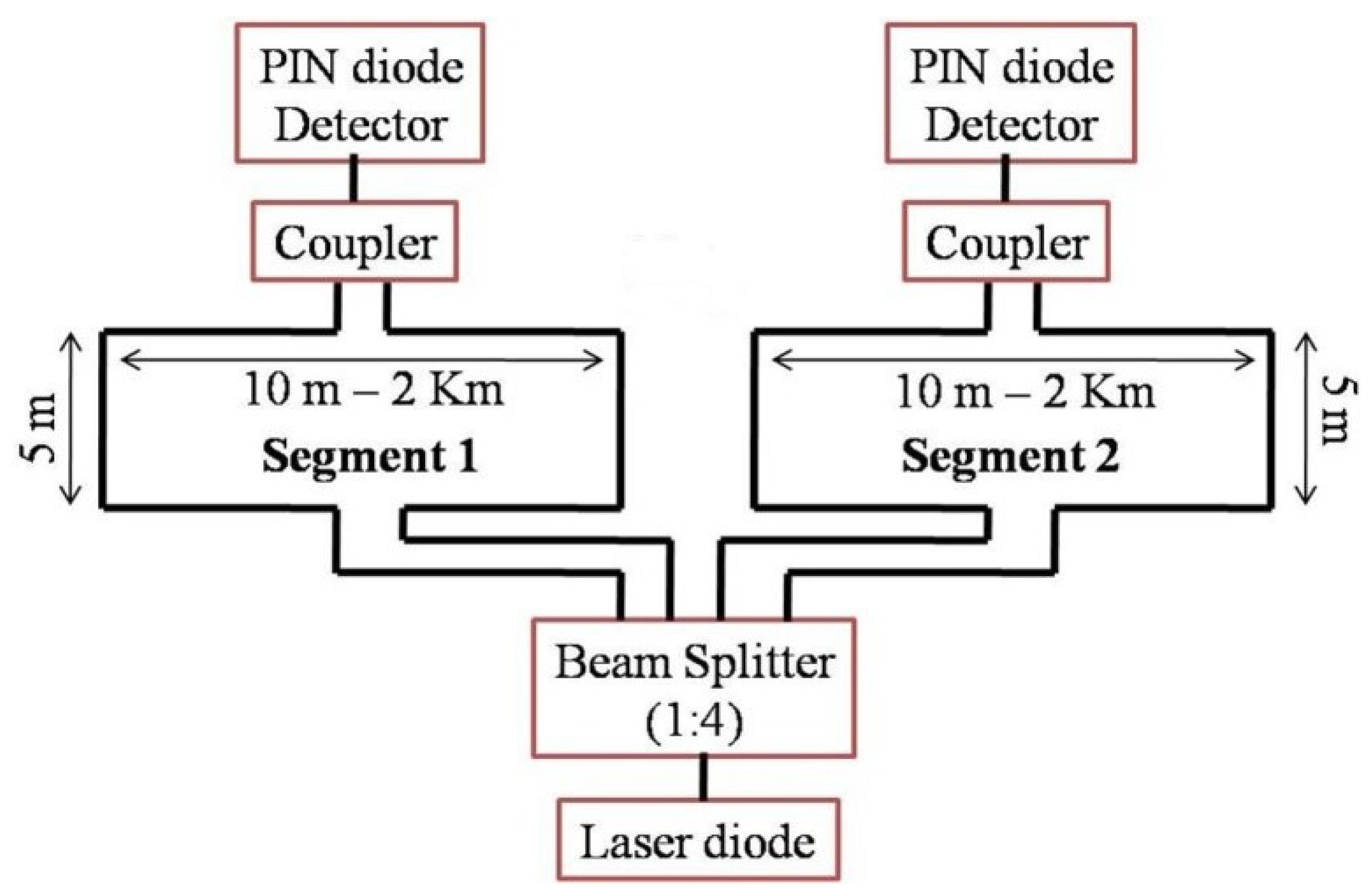
Figure 1 shows the layout of a single area of the optical fiber sensor used to collect the signal. Each area contains two sections [11]. Two segments are used to locate the intruder. Two single-mode fiber optics separated by a distance of 5 m and buried at a depth of approximately 12 inches in the ground were used for each segment. The length of the optical fiber segments may vary from 10 m to 2 km depending on the requirements. Each segment has the capability of detecting and identifying the intruder walking on the buried fiber segment. Next, they send a message about the intruder and the segment number on a copper line to a mote.
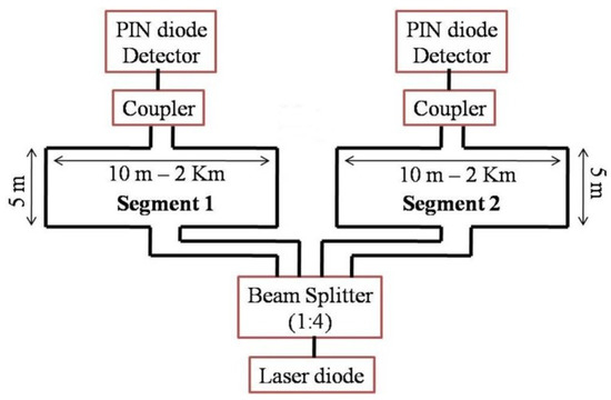
Figure 1.
Experimental setup of single fiber zone.
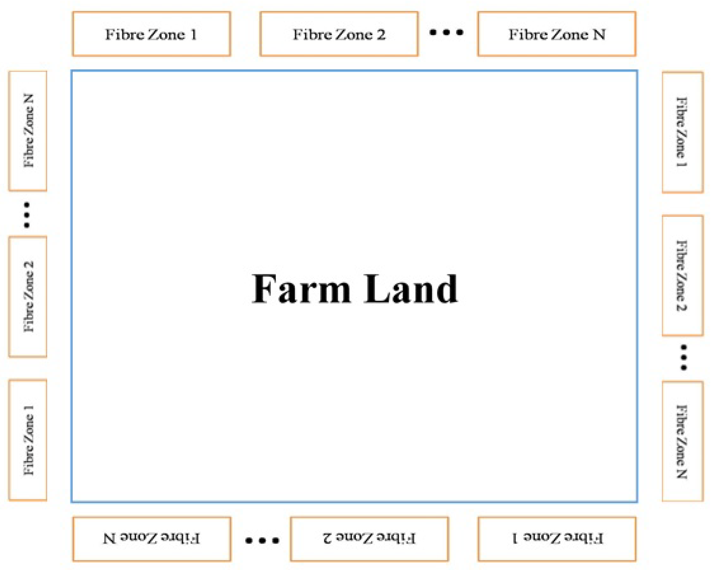
At the starting point, an IR laser beam is inserted to the fiber cable. The IR beam is split using a beam splitter (1:4), so that it can be inserted into four fiber cables simultaneously. At the receiving end, a PIN diode receives the signals and transmits to the processor (ARM processor). Figure 2 illustrates the arrangement of the areas around the farm. Different areas of fiber may be placed next to each other to cover more surface. Each fiber segment is identified and accompanied by event information to communicate the crossing location.
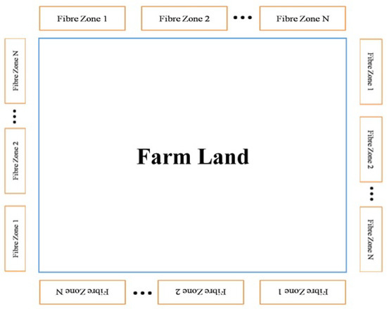
Figure 2.
Arrangement of fiber zones in farmland.
We concentrated on approaching the animal to identify the animal that came in without permission. The PIN LED signal is invariant to the depth of deployment, the nature of the ground, the weight of the animal, and the velocity of the movement of the animal.
2.2. Optical Fiber Cable
The world of broadcasting communications is rapidly changing from copper link organizations to optical fiber [12,13]. Optical filaments are an extremely fragile strand of non-terni glass that operates as waveguides to illuminate over significant distances. There are two principals of fiber optic links: monomode fiber (SMF) and multimode fiber (MMF). The principal distinction is in the part size. The MMF has a larger center, empowering the spread of various light modes (or ‘beams’). SMF has an extremely thin center that takes into consideration only one method of light dissemination. Each type of fiber has various properties with its own advantages and disadvantages. The optical fiber link can be used in a variety of situations. Some salient properties of the optical fiber link are as follows [14]:
- Their data are essentially boundless.
- They have a significant burden bearing limit.
- Their transmission errors are extremely low.
- They do not vent heat.
- They are shielded from electromagnetic impedance.
Fiber optic links have numerous applications in different modern circumstances. Some of them are mentioned below:
- Medical: Optical strands are adjusted to clinical use. They can be made of delicate and very meager strands to embed into the lungs, veins, and many empty pieces of the body. These fiber optics are utilized in various instruments that permit doctors to notice the inward pieces of the body without performing a medical procedure.
- Telecommunications: Fiber optics are introduced and utilized in gathering and transmission. Phone transmission depends on fiber optic links. These strands pass on energy by beats of light. Its innovation is similar to that of coaxial links; then again, actually optical fiber can handle a large number of discussions simultaneously.
- Networking: Fiber optics are utilized to interface workers and clients in an assortment of organization settings and furthermore help with expanding the exactness and speed of information transmission.
- Industrial/Commercial: Fibers are utilized for imaging in range regions, such as tangible gadgets for determining the temperature, such as cabling, where EMI is an issue, pressure, such as cabling in mechanical conditions and vehicles. TV Broadcasting/CATV Cable organizations use fiber-to-fiber cabling for superior quality TV, CATV, video-on-request, Internet, and numerous different applications.
- Defense/Government: They fill in as hydrophone for SONAR and seismic applications, in subs, airplane, and other vehicle wiring.
- Data Storage: Fiber optic links are used for information stockpiling and transmission. Fiber optic links are additionally utilized for imaging and lighting purposes and as sensors for observing and estimating a wide scope of factors. Moreover, fiber optic links are utilized in the turn of events, exploration, and testing of all the previously mentioned applications.
3. Signal Analysis
The signal classification is based on ground vibration and ground stress. The experimental configuration of the fiber optic sensor produces a frequency signal of approximately 400 Hz when the human or animal crosses it. This frequency is much lower compared to other ground vibrations such as vehicular passage and soil excavation, etc. The signals were recorded in various locations (such as the zoo, forests, open lands, etc.). Each signal has different features that are affected by the state of the ground, the depth of the optical fiber sensor in the ground, the gait of the animals, etc. The following signal retrieval techniques are used for signal analysis:
- First, signals were recorded without any motion on an optical fiber sensor (Figure 3).
 Figure 3. Threshold setting for noise removal (threshold level = 0.25).
 - The threshold value was calculated from the previous signal.
- Signal information about the events was recorded (Figure 4).
 Figure 4. Noise level.
 - Discard signals with an amplitude below the threshold and retrieve signals with an amplitude greater than the threshold. Figure 5 shows the de-noised signal. The de-noised signals are the events signals.
 Figure 5. De-noised (Event) signal.
Figure 3 represents the signal that is registered with few movement on the fiber sensor to find out the level of noise. The recorded signals shows the default vibrations on the ground with a few spikes of footsteps. The amplitude of the signal is found to be less than 0.13 v. In that case, the threshold for the noise is set at 0.13 v.
Figure 4 shows the signal for the noise.
Figure 5 shows the signal given after removing the low-level noise. All values lower than the threshold value (0.13) turn to zero. Now, only occurrence information is present in the signal. The occurrence signals were separated and analyzed for signal characteristics.
Following an investigation of different signs, it was seen that no decent model or envelope was found. This is the justification for why, as per different works, 15 boundaries were distinguished, which are valuable to perceive the type of animals introduced in Table 1. These components were stored in the essential dataset for each sign and utilized in executing the acknowledgment calculation.

Table 1.
List of features for accident detection.
Other than the above-described features, MFCC was also used for classification. The qualities of the mel frequency cepstral coefficients (MFCC) stand apart among the attributes most commonly utilized in acoustic signal processing. The process of MFCC (represented in Figure 6) from the signal is as follows:

Figure 6.
Mel Frequency Cepstral Coefficients (MFCC) block diagram.
- 1.
- Input Digital Signal Windowing: Handling an enormous dataset is troublesome. To comprehend the sign model and examine it, an enormous dataset is separated into various pictures, known as windowing.
- 2.
- Carry out a Discrete Fourier (DFT) transform of every window to ascertain the frequency range of a sign.
- 3.
- Rewind the yield of the second stage with mel-frequency channel bank.
- 4.
- Apply the logarithm toward the end of the third stage.
- 5.
- Calculate the Inverse Discrete Fourier Transform (IDFT) of log yield.
- 6.
- Calculate the Discrete Cosine Transform (DCT) of the IDFT yield to pack the sign.
- 7.
- When delivered, an incentive for every window will be produced.
Table 2 presents the data extracted for six animal crossing signals.

Table 2.
Numeric values of the collected features.
The signs have been recorded in various places (such as the zoo, forests, open lands, etc.). Each signal has different characteristics that are affected by the condition of the ground, the depth of the optical fiber sensor in the ground, the gait of the animals, etc. To observe the signal model for different classes, the signals have been divided into multiple frames (window), and the frame size is calculated by dividing the whole signal.
We attempted to find a model by dividing the signal time of the event by 10, 15, 20, and 25. We split that signal by 15. After splitting the event signals into 15 images, the RMS value for each image was calculated. These RMS values were stored in the main database and used to analyze the signal template. An event signal may have two or more event signatures.
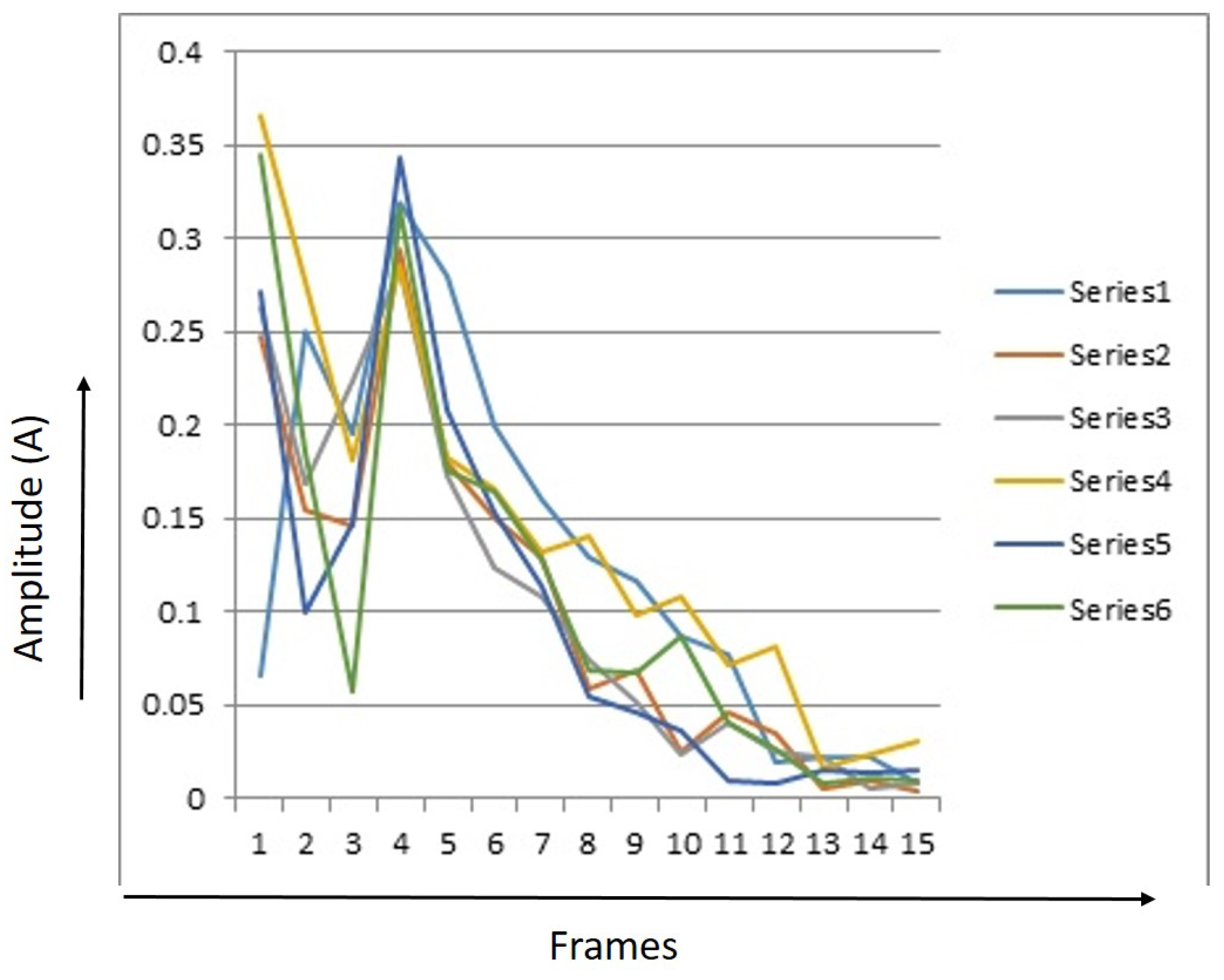
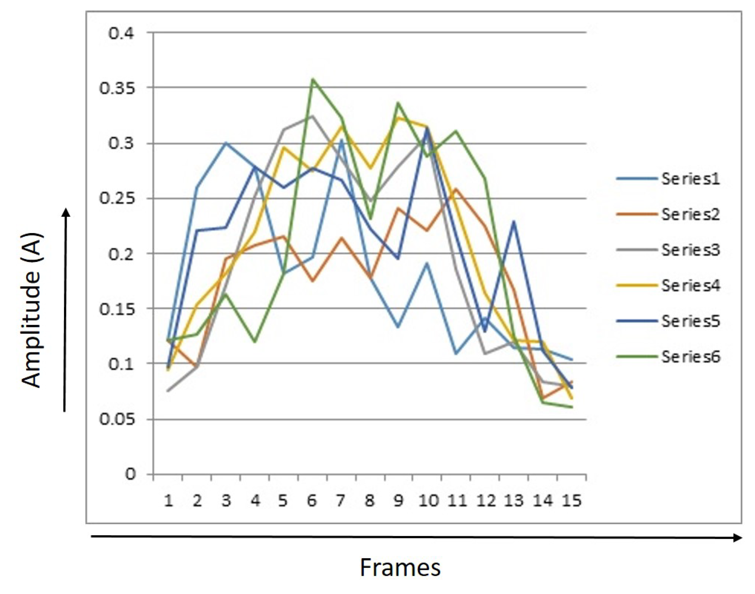
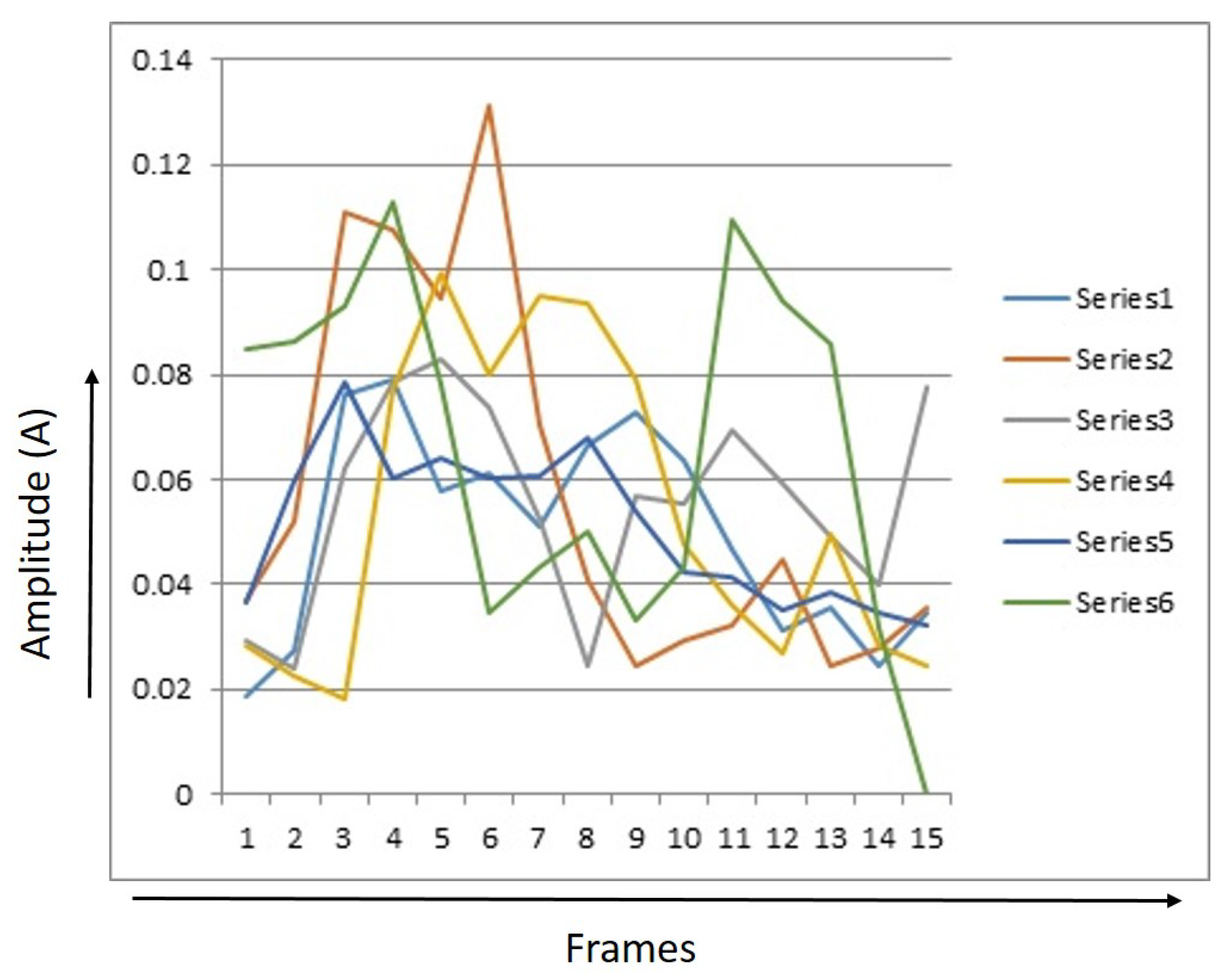
Every signature had 15 RMS values. The RMS value for each image was saved separately for several signals. Figure 7, Figure 8 and Figure 9 provide RMS values of 15 points for humans, tigers, and elephants for six different signals. The x-axis shows the number of frames and the y-axis shows the RMS value for six samples. The graph illustrates a trend that identifies different classes.
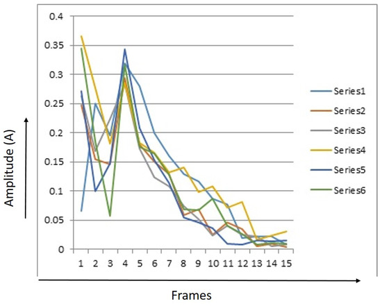
Figure 7.
15 Points Root Mean Square (RMS) values of 6 event signals of humans.

Figure 8.
15 Point RMS values of 6 event signals of elephants.
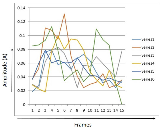
Figure 9.
15 Point RMS values of 6 event signals of tigers.
Figure 7 shows a graph with 15 point RMS values for humans. It can be seen that the energy level of most signals taken for humans is between 0.24 and 0.37. After that, it comes down. After the rise, the energy level declines continuously. This plot shows the model of a human gait.
Figure 8 shows a graphic of the 15 point RMS values for elephants. The energy level of most of the signals taken for the elephant can be observed to be between 0.07 and 0.13. After that, energy level goes up. After passing the power level of the fiber optic cable, the signal goes down again and its range is 0.06 to 0.11.
Figure 9 shows a graph of RMS values of 15 dots for tigers. One can observe that the energy level of the signal increases when the tiger approaches the optical fiber sensor. The signal features a small rise at the beginning and then a sudden rise, after that it goes down, then a small rise and fall until the end. The pads of the tiger foot are very soft, so it applies a very small amount of pressure to the fiber cable—that is why the RMS energy level of signature varies from 0 to 0.13
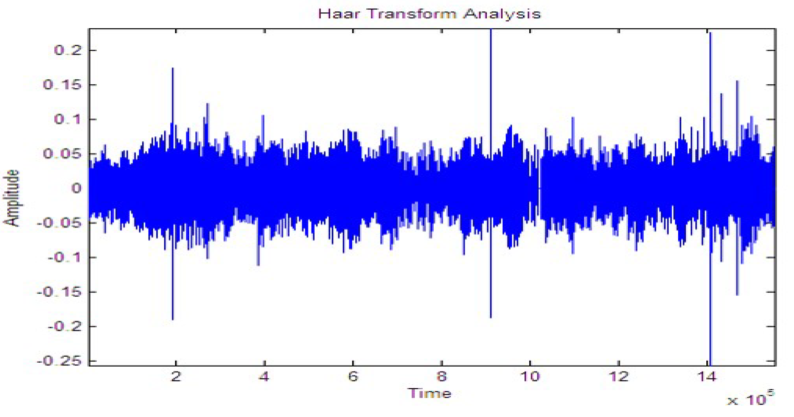
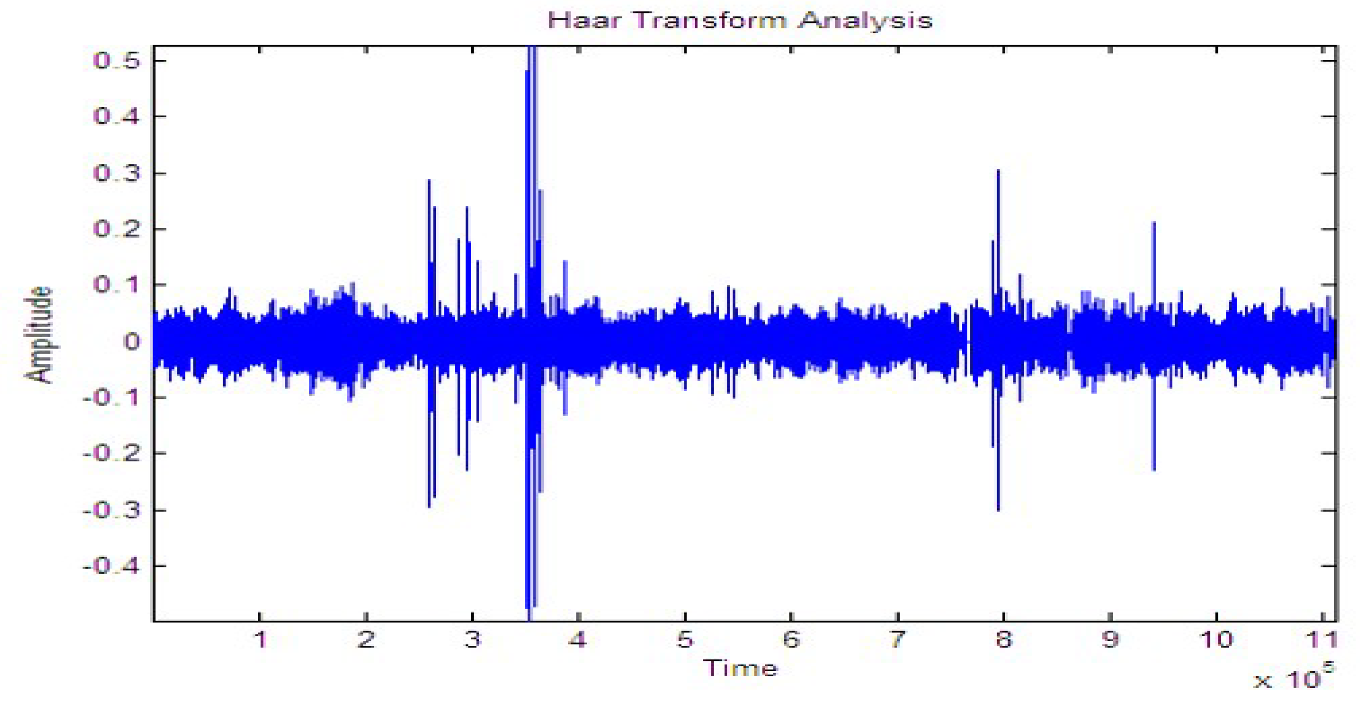
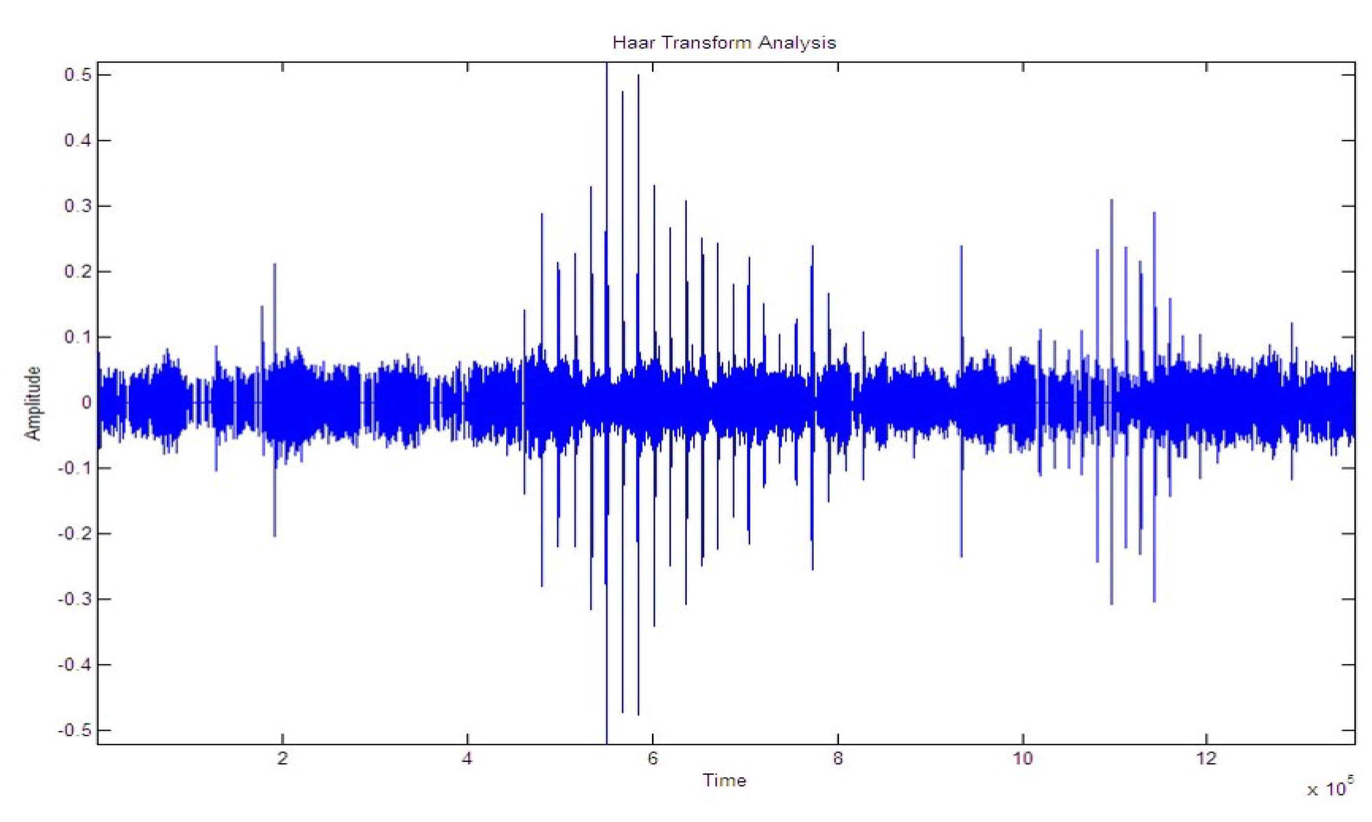
Figure 10, Figure 11 and Figure 12 shows the signal for the motion of several people over a buried fiber cable. The observation of the magnitude increase for walking, running, tapping performed across the cables is illustrated in Table 3.

Figure 10.
Signal while walking.

Figure 11.
Signal while running.
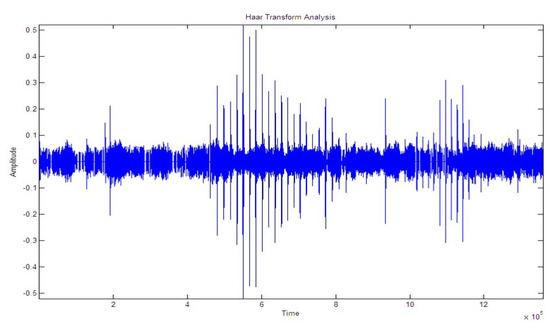
Figure 12.
Signal while tapping.

Table 3.
Observation of amplitude for signal.
Figure 13, Figure 14 and Figure 15 shows the signal for the motion of several people over a buried fiber cable. The observation of the magnitude increase for walking, running, tapping performed across the cables is illustrated in Table 4.
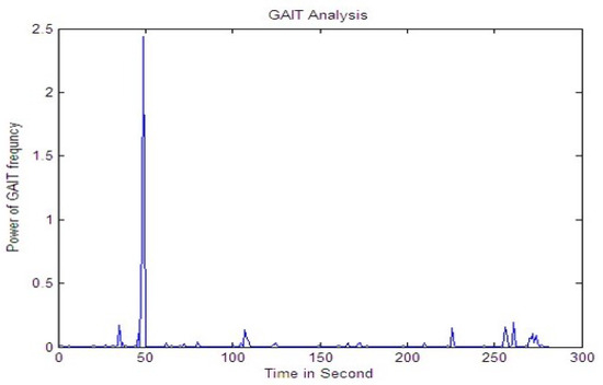
Figure 13.
Signal while walking.
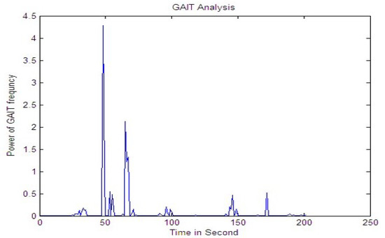
Figure 14.
Signal while running.

Figure 15.
Signal while tapping.

Table 4.
Observation of amplitude for signal.
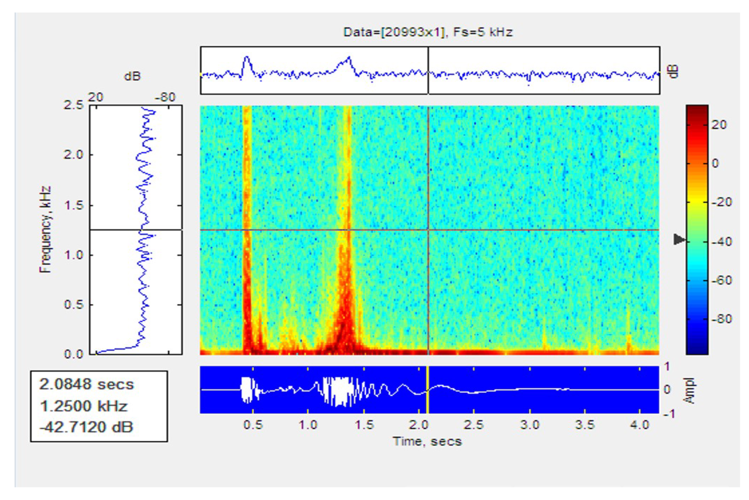
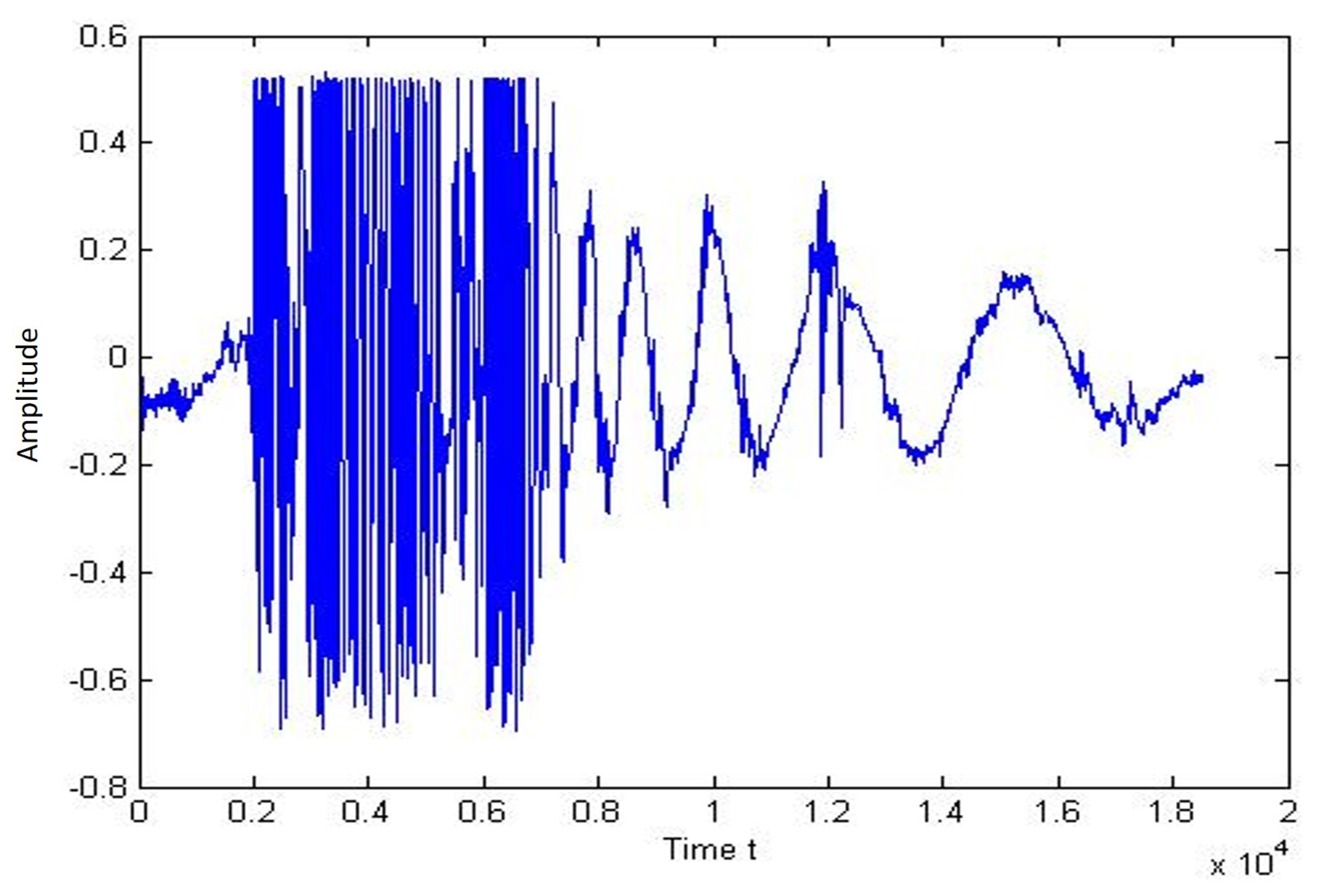
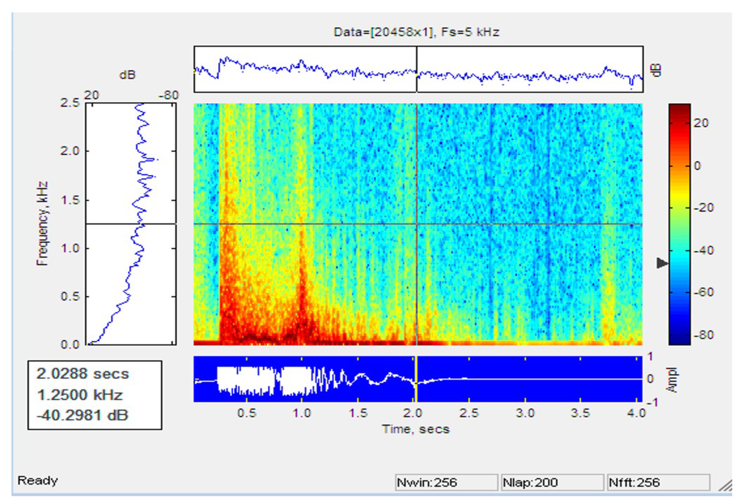
Figure 16 and Figure 17 shows the signal path and the spectrogram of a one-person walk. It can be seen in the graph that there is a peak when the person places their feet on the cable.
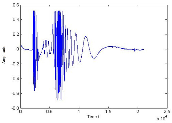
Figure 16.
Plot of signal for the walk of a single person.
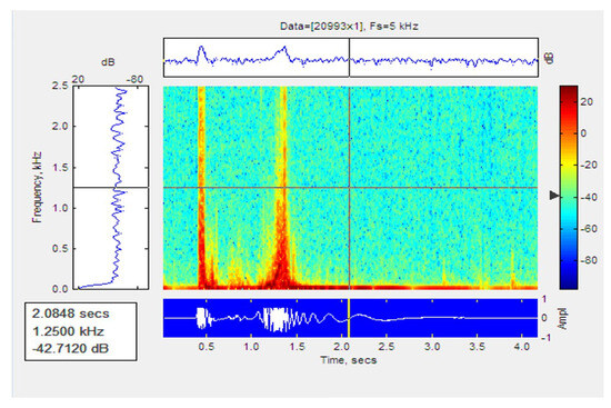
Figure 17.
Spectogram of signal for the walk of a single person.
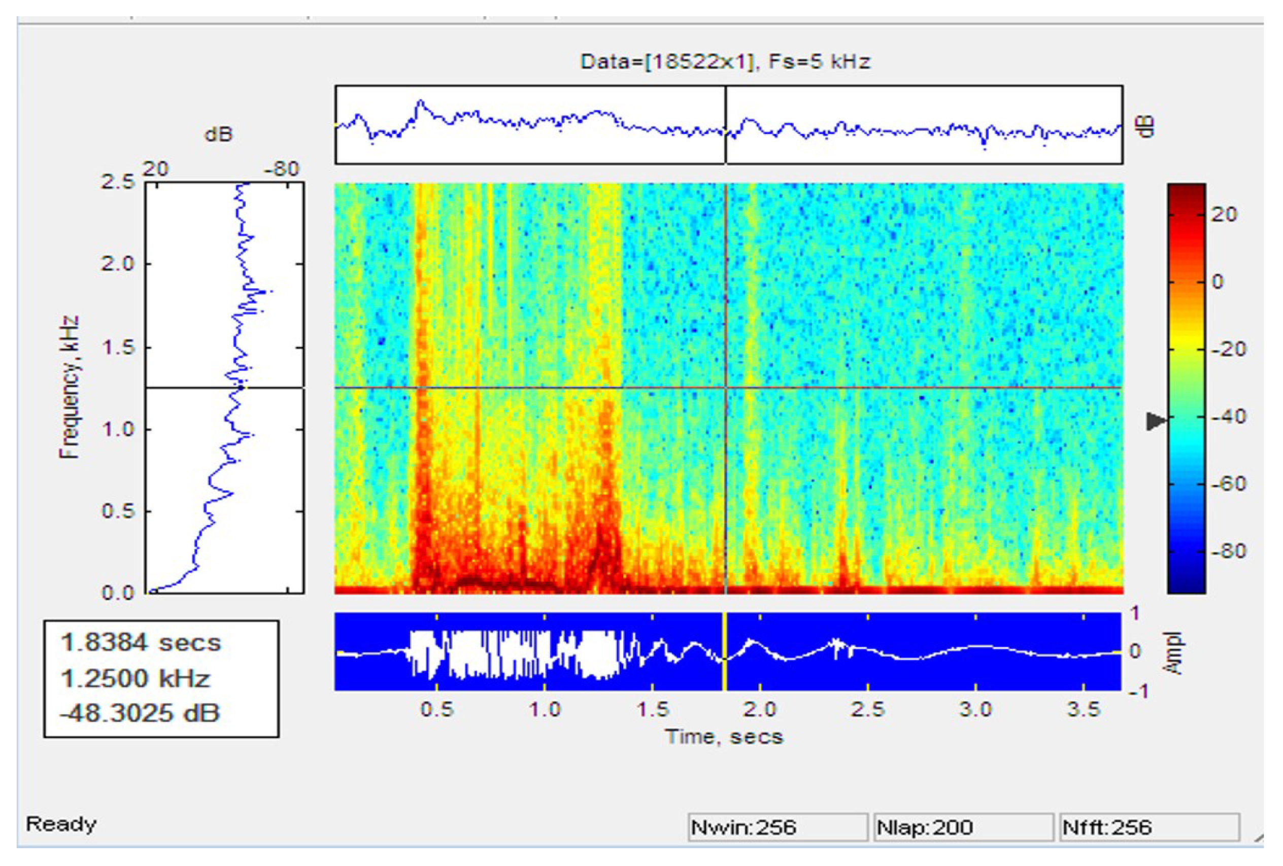
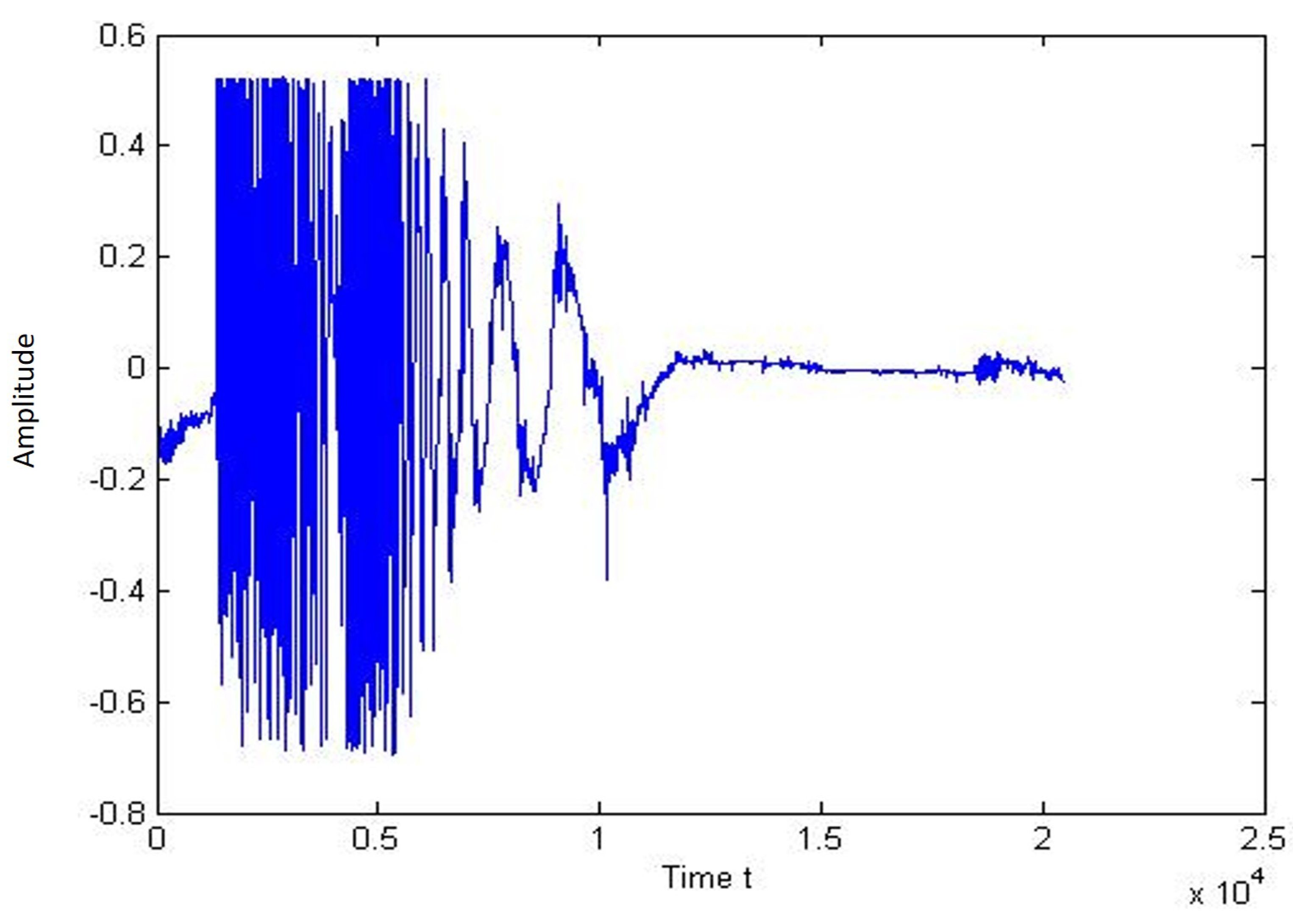
Figure 18 and Figure 19 shows the signal pattern and the single-person performance spectrogram. The graph shows a peak when the person reaches the nearby cable and crosses the sensor cable.
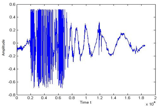
Figure 18.
Plot of signal for running of single person.
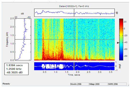
Figure 19.
Spectogram of signal for running of single person.
Figure 20 and Figure 21 represent the signal trace and the one-person jump spectrogram. It can be seen from the chart that there is a peak when the person jumps close to the sensor cable.
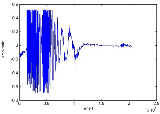
Figure 20.
Plot of signal for jump of single person.
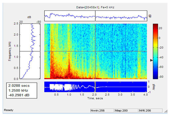
Figure 21.
Spectogram of signal for jump of single person.
4. Algorithm for Classification
The first algorithm is based upon the table of RMS values at each signal point. The threshold has two tiers. The first threshold layer is defined as the average of the RMS combined with a standard deviation. The lower end of the RMS is defined as the mean of the RMS value less than SD. The second cut-off layer is defined as the mean of the RMS values plus the 2X standard deviation. In this case, the lower limit is defined as the mean of the RMS value minus two times the standard deviation. The classification algorithm is based on the number of points passing through both frontiers. The steps for establishing thresholds are as follows:
- a.
- Calculated average of RMS per image for multi-event signal.
- b.
- Calculated standard deviation (Sigma) for each field for two or more event signals.
- c.
- Create threshold boundaries by averaging RMS values for each image, standard deviation (sigma) for each image, average sigma, average sigma, average sigma 2 * sigma, average sigma − 2 * sigma.
- d.
- The classification of intruder is based on number of points that lie between the first boundary of average + sigma & average − sigma, and second boundary of average + 2 * sigma & average − 2 * sigma.
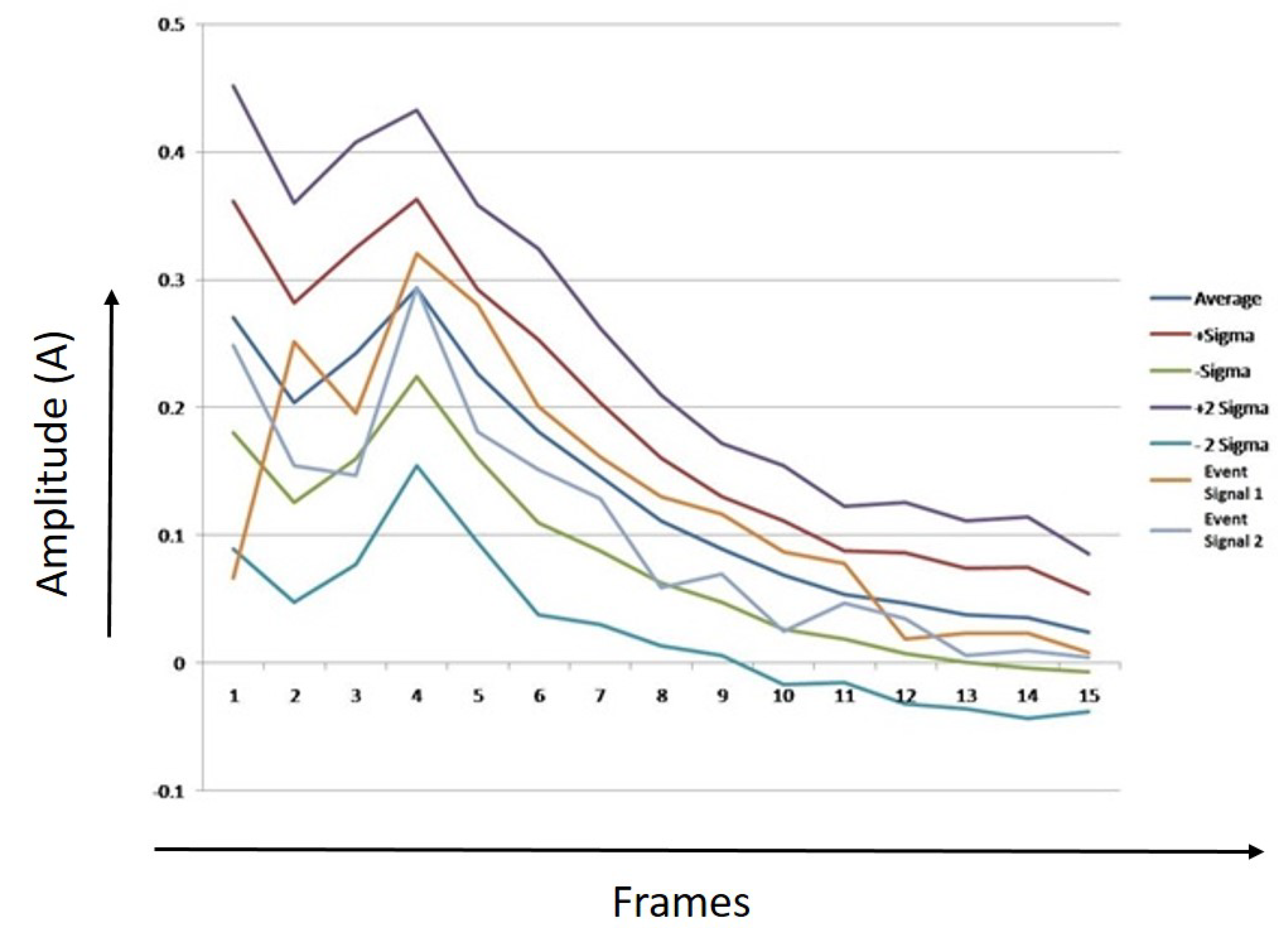
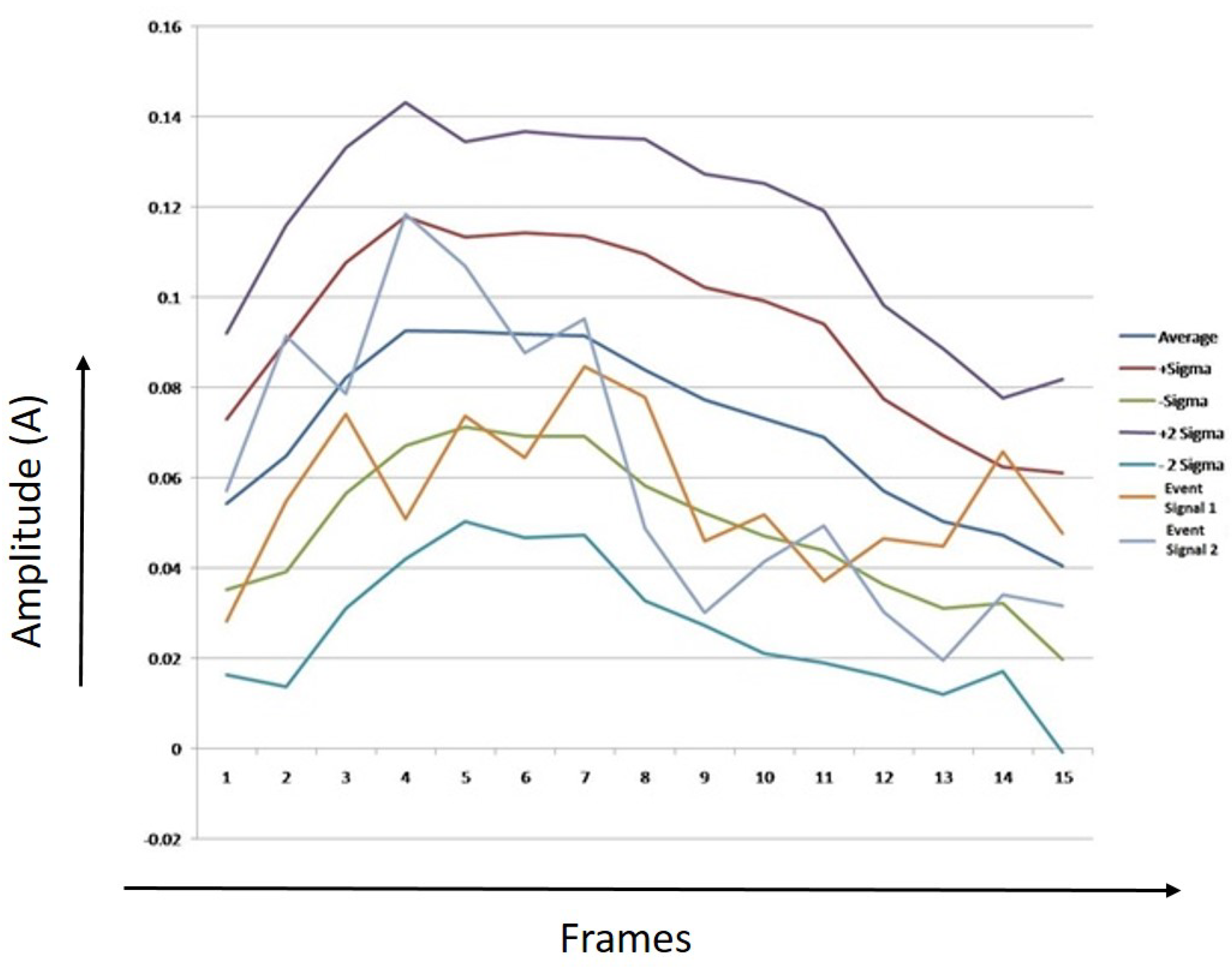
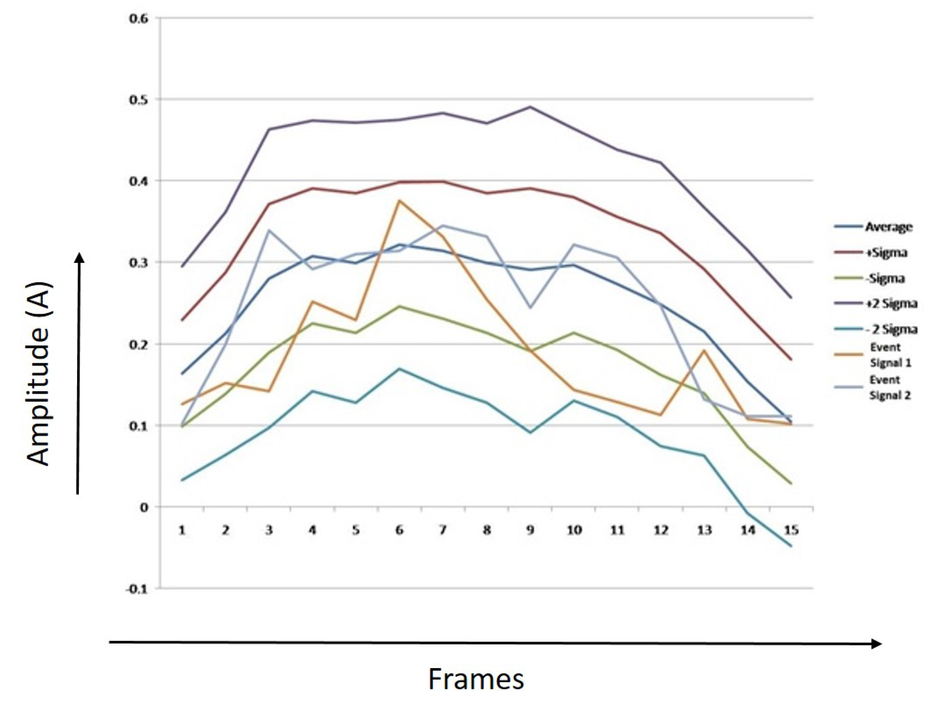
Figure 22, Figure 23 and Figure 24 show thresholds for humans, tigers, and elephants. The mean RMS values and the sample of two event signals for each class are also shown in the chart. X-axis represents the number of frames, Y-axis represents the values of average of RMS, first threshold boundary (average + sigma & average − Sigma), second threshold boundary (average + 2 * sigma & average − 2 * Sigma), and RMS values of two event signals.
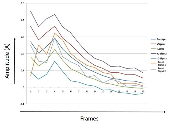
Figure 22.
Threshold boundaries for human.
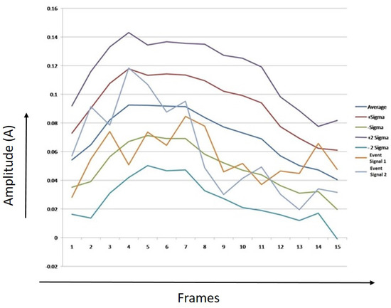
Figure 23.
Threshold boundaries for tiger.
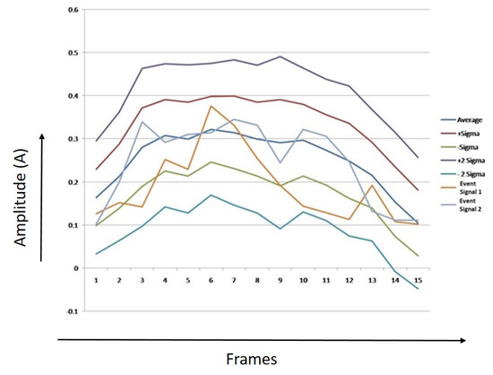
Figure 24.
Threshold boundaries for elephant.
It can be observed from Figure 22, Figure 23 and Figure 24 that most of the points of sample 1 and 2 lie between the first threshold boundaries, and few points lay between the second threshold boundaries. The algorithm was developed after analyzing and counting the number of dots that lie between the limits.
4.1. K-Means Clustering
K-means clustering serves to shape the framework for distinguishing and perceiving occasions. The calculation is as follows:
- Stage 1:
- Create an information base by considering the signal acknowledgment to be variable from the training set.
- Stage 2:
- Establish a bunch of focuses arbitrarily from the preparation bundle.
- Stage 3:
- Test and endeavor to group signals in the general arrangement.
- Stage 4:
- For every Xi model in the preparation bundle, find the closest C* bunch focus and rank Xi as a C* part.
- Stage 5:
- For each bunch, recalculate its middle by discovering a group normal.
- Stage 6:
- If the number of cluster centers is lower than the specified number, divide each cluster center into two clusters by finding the entry dimension with the highest gap.
Testing: For each pattern X, associate X with the cluster Y closest to X using the Euclidean distance
4.2. Decision Tree with Filters
The decision tree is a controlled learning strategy for various arrangements. It takes choices as per replacement cases and if–else presentations. More precise grouping results are controlled by tree profundity. The decision tree is a tree structure that permits order and relapse. It breaks dataset into a few subsets and constructs a chain of command. The bunches of the leaves are the final product of the tree. Contingent upon the tree format of the affiliation rules can be extended. These coordinating with rules might be carried out on any of the coding languages and gadgets.
The calculation utilized for this paper is an expansion of the decision tree, and used to build the accuracy of the acknowledgment. In this strategy, all signs were isolated into four frequency bands. The frequency bands include:
- First low-pass channel 5 KHz.
- Second band pass channel 5–10 KHz.
- Third channel pass channel 10–15 KHz.
- Fourth high stream channel >15 KHz.
Every one of the 15 boundaries were determined for each band of sign. In this manner, 50 upsides of every boundary for each sign were determined and put away in the dataset. After the production of the dataset, the decision tree is applied. The decision tree produced affiliation rules with the most prevailing aspect set. As indicated by affiliation rules, the choice for the occasion has been taken.
The information sound sign is enhanced and separated through proper circuits after the condition signal is given to the microcontroller.
At the end, the three calculations provide an exit on the grounds that the sign is an occasion (vehicle mishap) or not (Figure 25). On the off-chance that the sign is an occasion, the yield will be Y or N. The larger part meter will count both Y and N. On the off-chance that the quantity of Y is more noteworthy than or equivalent to 2, the ultimate result will be pronounced as Event Detected. An itemized clarification of the calculation is introduced in the accompanying area.
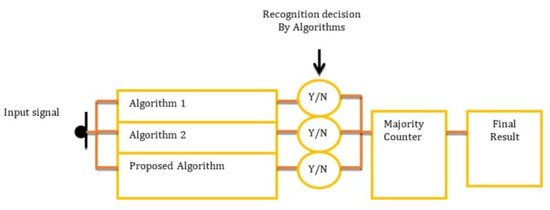
Figure 25.
Flow chart of the combined system.
5. Results
The complete setup of the optical fiber cable sensor has been tested in a regressed manner. The testing was performed for the identification of humans, tigers, and elephants. The identification of humans was performed in the farms where a complete setup was deployed. Three sets of humans (50 person in each set) walked randomly on the deployed setup. The persons used for testing was not included for the data collection for training.
The second test was performed for the identification of elephants, because many farms are destroyed by elephants. Three pet elephants were rented and tested on the same setup that was used for humans. All four elephants crossed the setup in a random manner (single elephants and in groups). A total of 85 elephant crossings were tested.
The third test was performed for tigers in the zoo. The setup was deployed in the movement area of the tigers. Three different tigers were selected for the testing purpose. A camera was placed for ground truth verification and to count the crossings of the tigers. The setup was fixed for 15 days, where 115 crossings of tiger was recorded.
There have been very few instances where the algorithm has been unable to identify the type of animal. The efficiency of the result is shown in Table 5, and we consider them quite promising.

Table 5.
Test results for three datasets.
6. Conclusions
Fences are incredibly important for the security of farmland. Wild animals cause damage to crops, which causes damages to the finances of farmers. Every farmer builds fences before they begin farming. Farmers depend on many kinds of fences. A few of them are truly dangerous to animals. The unsafe use of fences kill animals relatively frequently—according to records gathered by a few organizations, a large number of elephants, cows, and other animals die every year.
In this paper, we proposed a virtual fencing using a fiber optic sensor. The virtual fence is smart enough to identify the animals. Following the identification of the animals, it can send a message to the owner of the farm and generate an alarm.
The smart fence presented in the paper used machine learning algorithms that are effective in identifying signals unique to humans, elephants, and tigers. Other than identification of specified animals, the smart fence is currently able to recognize the movement of anyone around the farmland.
The complete configuration of the optical fiber cable sensor was tested very regressively. Tests have been carried out to identify humans, tigers, and elephants. Human identification was conducted at farms where the full configuration was deployed. Three sets of humans (50 persons in each set) were moved randomly on the deployed configuration. The individuals used for the tests were not taken into account for the collection of training data. The efficiency of the system is 94–96% for identification of humans.
A second test was carried out to identify elephants because plenty of farms are destroyed by elephants. Three pet elephants were hired on the same configuration that was used for humans. All four elephants were randomly intersected (one elephant and in groups). There were 85 elephant crossings tested. The efficiency of the system is 75% for identification of elephants.
The third test was carried out on tigers at the zoo. The configuration has been deployed in the tiger’s motion zone. A camera was placed to check the truth on the field and count tiger passes. Three different tigers were used for testing purposes. The facility was repaired for 15 days, while 115 crossings on the tiger were recorded. The efficiency of system is 80% for identification of tigers.
Very few cases were found where the algorithm was unable to identify the type of animal. The efficiency of the result is shown in Table 5, and are promising. This setup will be very useful for farmers; they can save their crops without harming animals.
The future research will be focused on identifying more animals and the development of a deterrent fence to repel animal incursions into the farm. The deterrent fence will consist of drum noises, honeybee attacks, or smells disliked by animals. The smart fence can be further developed into a closed area monitoring system. In the future, the results will also be gathered for different ambiance and temperatures.
Author Contributions
Conceptualization, P.S., F.R.A. and M.S.; Data curation, D.K.S.; Formal analysis, D.K.S., F.R.A. and M.S.; Funding acquisition, F.R.A.; Investigation, F.R.A.; Methodology, P.S., D.K.S., F.R.A. and M.S.; Project administration, P.S. and D.K.S.; Resources, D.K.S. and M.S.; Software, D.K.S.; Validation, P.S., F.R.A. and M.S.; Writing—original draft, D.K.S.; Writing—review and editing, P.S., F.R.A. and M.S. All authors have read and agreed to the published version of the manuscript.
Funding
The research is supported by Taif University, Taif, Saudi Arabia, and belongs to Project Number(TURSP-2020/331), Taif University, Taif, Saudi Arabia.
Acknowledgments
The authors would like to acknowledge the support from Taif University Researchers Supporting Project Number(TURSP-2020/331), Taif University, Taif, Saudi Arabia.
Conflicts of Interest
The authors declare no conflict of interest.
Correctioin Statement
This article has been republished with a minor correction to resolve spelling and grammatical errors. This change does not affect the scientific content of the article.
References
- Agrifarming. Available online: https://blog.apnikheti.com/agriculture-problems-and-their-solutions/ (accessed on 16 August 2021).
- Suman, S. Indian Agriculture Problems: 7 Major Problems of Indian Agriculture, Economic Discussions (Blog). Available online: https://www.economicsdiscussion.net/agriculture/problems-agriculture/indian-agriculture-problems-7-major-problemsof-indian-agriculture/12859 (accessed on 14 August 2021).
- Pradhan, S. Problems Faced by Farmers in India. Pscnotes (Blog), 6 May 2020. Available online: https://pscnotes.in/problems-faced-by-farmers-in-india/ (accessed on 5 August 2021).
- Mathrubhumi. Available online: https://english.mathrubhumi.com/news/kerala/553-animals-killed-by-electrocution-during-last-10-years-1.4421023 (accessed on 10 August 2021).
- Mistry, K. 11 Different Types of Fences that Are Widely Used around your Home Gharpedia (Blog). Available online: https://gharpedia.com/blog/11-types-of-fences/ (accessed on 13 August 2021).
- Home Stratosphere. Available online: https://www.homestratosphere.com/types-of-wire-fencing/ (accessed on 21 August 2021).
- Florida State Fence. Available online: https://www.floridastatefence.com/2019/05/01/the-9-types-of-fences-which-type-of-fence-do-you-need/ (accessed on 15 August 2021).
- Huchtkoetter, J.; Reinhardt, A. Demo: Taking Advantage of the Shock Hazard: How to Use an Electric Fence for Data Transfers. In Proceedings of the 2018 14th International Conference on Distributed Computing in Sensor Systems (DCOSS), New York, NY, USA, 18–20 June 2018; pp. 117–118. [Google Scholar]
- Firdhous, M.F.M. IoT-enhanced Smart Laser Fence for Reducing Human Elephant Conflicts. In Proceedings of the 2020 5th International Conference on Information Technology Research (ICITR), Moratuwa, Sri Lanka, 2–4 December 2020; pp. 1–5. [Google Scholar]
- Chen, L.; O’Keeffe, S.; Woulfe, P.; Lewis, E. A comparison of clinic based dosimeters based on silica optical fibre and plastic optical fibre for in-vivo dosimetry. In Proceedings of the 2017 25th Optical Fiber Sensors Conference (OFS), Jeju, Korea, 24–28 April 2017; pp. 1–4. [Google Scholar]
- Memon, S.F.; Lewis, E.; Pembroke, J.T.; Chowdhry, B.S. A novel inter-fibre light coupling sensor probe using plastic optical fibre for ethanol concentration monitoring at initial production rate. In Proceedings of the 2017 25th Optical Fiber Sensors Conference (OFS), Jeju, Korea, 24–28 April 2017; pp. 1–4. [Google Scholar]
- Shoaie, M.A.; Meroli, S.; Machado, S.; Ricci, D. Evolution of optical fibre cabling components at CERN: Performance and technology trends analysis. Opt. Fiber Technol. 2018, 42, 69–74. [Google Scholar] [CrossRef]
- Xu, X.; Liu, Y.; Gao, F.; Song, N. Phase sensitivity of fundamental mode to external atmospheric pressure for hollow-core photonic bandgap fiber. Opt. Fiber Technol. 2018, 43, 153–157. [Google Scholar] [CrossRef]
- Min, R.; Liu, Z.; Pereira, L.; Yang, C.; Sui, Q.; Marques, C. Optical fiber sensing for marine environment and marine structural health monitoring: A review. Opt. Laser Technol. 2021, 140, 107082. [Google Scholar] [CrossRef]
Publisher’s Note: MDPI stays neutral with regard to jurisdictional claims in published maps and institutional affiliations. |
© 2021 by the authors. Licensee MDPI, Basel, Switzerland. This article is an open access article distributed under the terms and conditions of the Creative Commons Attribution (CC BY) license (https://creativecommons.org/licenses/by/4.0/).

