PermLSTM: A High Energy-Efficiency LSTM Accelerator Architecture

Abstract

Pruning and quantization are two commonly used approaches to accelerate the LSTM (Long Short-Term Memory) model. However, the traditional linear quantization usually suffers from the problem of gradient vanishing, and the existing pruning methods all have the problem of producing undesired irregular sparsity or large indexing overhead. To alleviate the problem of vanishing gradient, this work proposed a normalized linear quantization approach, which first normalize operands regionally and then quantize them in a local mix-max range. To overcome the problem of irregular sparsity and large indexing overhead, this work adopts the permuted block diagonal mask matrices to generate the sparse model. Due to the sparse model being highly regular, the position of non-zero weights can be obtained by a simple calculation, thus avoiding the large indexing overhead. Based on the sparse LSTM model generated from the permuted block diagonal mask matrices, this paper also proposed a high energy-efficiency accelerator, PermLSTM that comprehensively exploits the sparsity of weights, activations, and products regarding the matrix–vector multiplications, resulting in a 55.1% reduction in power consumption. The accelerator has been realized on Arria-10 FPGAs running at 150 MHz and achieved $2.19\times$∼$24.4\times$ energy efficiency compared with the other FPGA-based LSTM accelerators previously reported.

1. Introduction

LSTM and GRU (Gated Recurrent Unit) are two most popular variants of RNN, which have been commonly applied in the sequence processing tasks [1,2,3,4]. Despite their superior capabilities in dealing with the dynamic temporal behavior of data sequences, those two architectures usually suffer from difficulties in the hardware design due to the presence of overwhelmingly numerous parameters and hence the occurrence of high computational complexity. In this work, we explore an avenue to minimize the inference part of the sparse LSTM model pruned by permuted diagonal mask matrices, so called PermLSTM, aiming for high processing performance as well as high energy-efficiency. The design methods derived from this study primarily on LTSM are also applicable to the case of the GRU, since both types of the network share the common architecture except that a GRU has two gates (reset and update gates), whereas an LSTM has three gates (namely input, output, and forget gates).

As suggested in Table 1 and Table 2, the power dissipated in accessing the off-chip memory is far more than the on-chip memory and, at the worst, those floating-point operations are extremely power hungry. Therefore, by compressing the network model in an appropriate way, the power dissipation can be reduced without necessarily degrading the whole system. This paper presents a hardware-friendly pruning approach that uses the permuted block diagonal mask matrix to generate a regular sparse structure. Differing from the previous approaches, our processing method completely eliminates some excessive indexing overhead in tracking of non-zero values, which lessens the computational load for hardware implementation. Quantifying weights and activations to fixed-point numbers should also compress the model. However, the linear quantization without normalization usually suffers from non-convergence problems literally caused by the saturation operations involved. To mitigate such a problem, this work proposed a linear quantization with local normalization to map the operands evenly over the range of [−1, 1]. It should be noted that, in order to reduce the impact of normalization on the accuracy of the model as much as possible, this work did not perform the global normalization on the operands, but adopted a more refined normalization approach, that is, grouping the operands according to the output result firstly, and then normalizing the weights and activation in each group. Thus, all the complex and energy-consuming floating-point operations are avoided yet with a negligible accuracy loss. The entire compression flow is as shown in Figure 1.

Table 1. Breakdown of the energy consumption for multiply-accumulate operations [5]. Adapted with permission from ref. [5]. Copyright 2014 IEEE.

Operation	Multiplication	Addition
8 bits Integers	0.2 pJ	0.03 pJ
32 bits Integers	3.1 pJ	0.1 pJ
16 bits Floating Point	1.1 pJ	0.4 pJ
32 bits Floating Point	3.7 pJ	0.9 pJ

Table 2. Breakdown of the energy consumption for memory access [5]. Adapted with permission from ref. [5]. Copyright 2014 IEEE.

Memory Size	64-Bit Memory Access
8 k	10 pJ
32 k	20 pJ
1 M	100 pJ
DRAM	1.3–2.6 nJ

Figure 1. The entire compression flow.

Implementation of those activation functions in LSTM is also cumbersome. In previous works, the activation function is often calculated based on the lookup table, the piecewise linear approximation or the curve fitting, giving rise to deteriorated network performance. As described in detail below, it has been found that properly tailoring the piecewise linear approximation to the quantization of the activation in terms of precision should help alleviate those shortcomings owing to some unreconciled error conflicts. Hence, such considerations have been incorporated into our design to boost the energy efficiency.

In addition to the optimization effort at algorithmic level, we also investigate into the design of an efficient processing unit to fully exploit the sparsity of the model. Most of the previous works have focused only on exploiting the sparsity on the weight and the activation. We further extend this sparsity exploitation to the product, which could also be sparse. In fact, as long as either a weight or an activation is zero, the resulting product will certainly be zero. Therefore, the product should have a degree of sparsity that is equivalent to or even greater than in the weight. By tapping into this property, we can effectively reduce the number of additions that follow. Provided that there was no new auxiliary circuitry being added, the power dissipation regarding the whole system then decreases. Since all the weights are pruned using the permuted block diagonal mask matrices, the position of a non-zero weight can be easily located, thereby making it possible to execute only those valid calculations as far as the product concerned.

The main contributions of the work are highlighted below:

• A hardware-friendly compression algorithm that combines both linear quantization with local normalization and structured pruning has been proposed. In comparison to the existing pruning approaches, it excels in dealing with processing irregularity and also in eliminating excessive indexing overhead. Similarly, in comparison to the existing quantization approaches, it not only solved the problem of vanishing gradient, but also adopted a more refined normalization approach to minimize the impact of normalization on model accuracy.
• The discrepancy arising from approximating the sigmoid function with the piecewise linear function has been defined and evaluated. Furthermore, an analysis is made to guide the selection of the bit-width of operands, in a way to facilitate the hardware implementation with minimum resources, as well as to retain the model accuracy.
• An energy-efficient accelerator architecture, PermLSTM, has been designed and implemented, to validate the proposed architecture which comprehensively exploits all sorts of the sparsity existing in the network.

The remainder of this paper is organized as follows: Section 2 gives a brief introduction on LSTM, followed by a quick overview on the existing pruning and quantization approaches. In Section 3, the proposed compression algorithm involving new strategies regarding structured pruning and linear quantization with local normalization is presented. Section 4 discusses our simplification effort in executing the activation functions. Section 5 further discusses design implementation for the proposed accelerator architecture. The experimental results are presented and compared in Section 6. Finally, conclusions are drawn in Section 7.

2. Background

2.1. Long Short-Term Memory

LSTM was first published by S. Hochreiter and J. Schmidhuber in 1997 [6] and later elaborated by F. Gers in 2002 [7]. For an LSTM, the input is characterized as a sequence of data that is: $\mathit{x}=(x_1,x_2,\dots ,x_n)$. Regarding a constituent unit in LSTM, the cell states $(\mathit{h},\mathit{c})$ and the internal gate $outputs\left(z\right)$ can be calculated by the following formulas:

$$\begin{array}{cc}\hfill {\mathit{z}}_t& =tanh({\mathit{w}}_x{\mathit{x}}_t+{\mathit{w}}_h{\mathit{h}}_{t-1}+\mathit{b})\hfill \end{array}$$

(1)

$$\begin{array}{cc}\hfill {\mathit{z}}_t^i& =\sigma ({\mathit{w}}_{ix}{\mathit{x}}_t+{\mathit{w}}_{ih}{\mathit{h}}_{t-1}+{\mathit{b}}_i)\hfill \end{array}$$

(2)

$$\begin{array}{cc}\hfill {\mathit{z}}_t^o& =\sigma ({\mathit{w}}_{ox}{\mathit{x}}_t+{\mathit{w}}_{oh}{\mathit{h}}_{t-1}+{\mathit{b}}_o)\hfill \end{array}$$

(3)

$$\begin{array}{cc}\hfill {\mathit{z}}_t^f& =\sigma ({\mathit{w}}_{fx}{\mathit{x}}_t+{\mathit{w}}_{fh}{\mathit{h}}_{t-1}+{\mathit{b}}_f)\hfill \end{array}$$

(4)

$$\begin{array}{cc}\hfill {\mathit{c}}_t& ={\mathit{z}}_t^f⨀{\mathit{c}}_{t-1}+{\mathit{z}}_t^i⨀{\mathit{z}}_t\hfill \end{array}$$

(5)

$$\begin{array}{cc}\hfill {\mathit{h}}_t& ={\mathit{z}}_t^o⨀tanh\left({\mathit{c}}_t\right)\hfill \end{array}$$

(6)

The superscriptions $i,f,o$ and the subscription t denote the input gate, the forget gate, the output gate, and the time step, respectively. Considering the input ${\mathit{x}}_tϵ{\mathbb{R}}^{n\times 1}$, the cell state ${\mathit{c}}_tϵ{\mathbb{R}}^{m\times 1}$ and the hidden state ${\mathit{h}}_tϵ{\mathbb{R}}^{m\times 1}$, we have a weight matrix for multiplication with the input data ${\mathit{w}}_{*x}ϵ{\mathbb{R}}^{m\times n}$, where $*ϵ\{i,o,f\}$. In addition, we have a weight matrix for multiplication with the hidden state ${\mathit{w}}_{*h}ϵ{\mathbb{R}}^{m\times m}$ and a bias vector ${\mathit{b}}_{*}ϵ{\mathbb{R}}^{m\times 1}$. The function $\sigma$ is regarded as a logistic sigmoid. The symbol ⨀ corresponds to an element-wise multiplication.

2.2. Model Compression

As some certain redundancy always exists in neural networks [8,9], pruning techniques have been proven effective in model compressing without necessarily degrading the performance. Unfortunately, the present weight pruning approaches all seem to have some drawbacks. Song. H. and Frederick. T. et al perform weight pruning by following the “smaller-norm-less-important” criterion, which suggests that weights with smaller norms can be pruned safely due to their insignificance [10,11,12,13]. Xin. D. and Pavlo. M. et al. heuristically search for trivial weights to be eliminated [14,15]. As illustrated in Figure 2b, these two approaches are generally prone to generating undesired irregular sparsity, which makes hardware design less efficient. Sharan. N. proposed the coarse-grained pruning method targeting all the weights in a block-manipulated fashion, surely delivering regular sparsity, but at the expense of the model accuracy (see Figure 2c) [16]. Referring to Figure 2d, Shi. C. divides each weight matrix row into a plurality of those equally sized banks (marked with different colors), and separately prunes each bank at fine-grained level [17]. This way, the same degree of sparsity across all the weight matrices can be obtained. Seyed. G. proposed a similar solution, which is pruning the model to obtain a row-balanced sparse matrix [18]. However, the address pointing to a non-zero weight position in their solutions becomes unpredictable and requires separate memory for storage.

Figure 2. The existing pruning methods illustrated by examples.

Quantization is another effective means in network compression. Itay. H. quantizes all the weights in binary, which has only two values, namely −1 and 1 [19]. In order to enhance the digital representation for better precision, Chenzhuo, Z. quantizes all the weights in ternary, yet still not sufficiently enough when dealing with some complicated tasks [20]. Shuchang. Z. devised some approaches of quantifying the weights and the activations to any-bit values [21]. In their approaches, an operand will be quantized within the range of $[-1+\Delta ,1-\Delta ]$ and otherwise saturated outside of this range. As shown in Figure 3a, for those operands far greater than 1 in value, even if the straight-through estimation [21] is applied regarding the gradient, such a way of truncation could still nullify some of the gradients according to our experimental results presented in Table 3, leaving the network hard to converge. As a consequence, this type of quantization is not performing well on some certain tasks. To rectify, Jungwook. C. proposed to limit activations within the range of $[0,2\alpha ]$, where $\alpha$ is a trainable parameter [22]. However, this approach is only applicable to the quantization of the activations rather than the weights.

Figure 3. (a) The linear quantization without normalization. (b) The linear quantization with local normalization.

Table 3. The perplexity of a model using two compression approaches with different bit-width.

$(\mathit{bitsW},\mathit{bitsA})$	Prune&NLQ	Prune&TLQ
(2, 8)	84.030	142.739
(4, 4)	58.930	113.929
(4, 6)	50.362	115.521
(4, 7)	45.926	115.276
(4, 8)	46.323	116.433
(8, 8)	45.742	120.141
Full precision	45.861	45.861

2.3. Hardware Acceleration

There are also many optimizations at the hardware level. Elham. A. use an approximate multiplier to replace the DSP block, thereby reducing the logic complexity and power consumption of the entire system [23,24]. Jo. J. measures how much the inputs of two adjacent LSTM cells are similar to each other, then disables the highly-similar LSTM operations and directly transfers the prior results for reducing the computational costs [25]. Patrick. J. use a shift-based arithmetic unit to perform multiplications in an arbitrary bit-width, aiming to make a full use of the properties offered by the low bit-width operands [26]. Bank-Tavakoli. E. optimized the pipeline of the datapath so that operations can be executed in parallel [27]. However, they stop short of exploiting the model sparsity. Jorge. A. tried to utilize only the sparsity in the weight during multiply-accumulate operations [28]. Shen. H. took advantage of the sparsity of both weight and activation [29,30]. In fact, there is a significant degree of sparsity also existing in the product, but, so far, there is no work utilizing this sparsity.

3. Hardware-Friendly Compression Algorithm

Pruning the network by using the permuted block diagonal mask matrices not only produces regular sparsity, but also eliminates the hardware overhead otherwise required to store the index regarding non-zero weights [31]. Quantization is another effective way of compressing the network. As mentioned earlier, the traditional linear quantization (TLQ) approach usually suffers from the non-convergence problem arising from the capped saturation. The normalized linear quantization (NLQ) approach, however, can, to a large extent, remove this limitation [32]. Accordingly, the entire training process will go through two phases. First, after pruned, the model is taken for training until it converges. Secondly, the model is subject to further quantization and then taken back for retraining until it converges once again.

3.1. Pruning the Network Using the Permuted Block Diagonal Mask Matrices

The permuted block diagonal mask matrix is defined as follows: for an m-by-n weight matrix $\mathit{w}ϵ{\mathbb{R}}^{m\times n}$, we have a mask matrix $\mathit{mask}ϵ{\mathbb{R}}^{m\times n}$, which contains $\frac{m}{p}\times \frac{n}{p}$ numbers of p-by-p sub-matrices. The elements of the mask matrix are defined as follows:

$$mas{k}_{ij}=\left\{\begin{array}{c}1if\left(\right(offset+c)modp=d)\hfill \\ 0otherwise\hfill \end{array}\right.$$

(7)

where $offset=\lfloor i/p\rfloor \times p+\lfloor j/p\rfloor$, $c=imodp$, $d=jmodp,$ and p is the rank of the sub-matrices. The $\frac{m}{p}\times \frac{n}{p}$ numbers of sub-matrices represent all the permuted block diagonal mask matrices used. Then, the pruned weight matrix ${\mathit{w}}^pϵ{\mathbb{R}}^{m\times n}$ can be obtained below:

$$w_{ij}^p=w_{ij}\times mas{k}_{ij}$$

(8)

Here, we give an example to illustrate how the network is pruned by the permuted mask matrix. For an 8-by-8 weight matrix as shown in Figure 4a, the rank of a mask sub-matrix is set to 4. According to the definition of the $offset$ given earlier, when the row index i and column index j, respectively range from 0 to 3, the $offset$ is 0. When $0\le i\le 3$ and $4\le j\le 7$, the $offset$ becomes 1. When $4\le i\le 7$ and $0\le j\le 3$, the $offset$ becomes 4. When $4\le i\le 7$ and $4\le j\le 7$, the $offset$ becomes 5. Substituting those four $offset$ values in (7), we will have the first and the third mask sub-matrices being of the identity matrix, and the second and the fourth mask sub-matrices can be acquired by cyclically right-shifting the first and the third mask sub-matrices, respectively. As a result, the pruned weight matrix is given in Figure 4b.

Figure 4. (a) An original weight matrix in high density. (b) Pruned by a permuted block-diagonal mask matrix with $p=4$.

3.2. Linear Quantization with Local Normalization

As shown in Figure 3a, any operand, whose value is less than 1, is quantized and otherwise saturated. Apparently, the associated quantization error will go up when the operand is getting far greater than 1, somehow causing the gradient to disappear during the training. To circumvent this problem, we map all the operands within the range of $[-1,1]$ prior to the quantization [32], as shown in Figure 4b. Instead of simply normalizing all the operands globally [33], the weights and the activations have been normalized separately in a more refined way.

For weights $\mathit{w}$ in LSTM, $\mathit{w}ϵ{\mathbb{R}}^{C_{in}\times C_{out}}$, where $C_{in}$ is the number of input channels, and $C_{out}$ is the number of output channels. Considering $a_j^{t+1}\propto {\sum }_{i=1}^{C_{in}}{w}_{ij}\times a_i^t\left(jϵ\{1,2,\dots ,C_{out}\}\right)$, it corresponds to the jth element in the activation vector and is evaluated at the (t + 1)th time step, having its associated calculations only related to those weights ${\mathit{w}}_{:,j}$ in the jth column of the weight matrix. Thus, the weights can be normalized per output channel. i.e.,

$$w_{ij}^n=\frac{w_{ij}}{max|{\mathit{w}}_{:,j}|}$$

(9)

For activations $\mathit{a}$ in LSTM, we have $\mathit{a}ϵ{\mathbb{R}}^{C_{in}\times 1}$. As, at the (t + 1)th time step, each element in the activation vector is iterated from all the elements in the last activation vector (i.e., at time step t), the normalized activations, ${\mathit{a}}^n$, can then be calculated below:

$$a_i^n=\frac{a_i}{max\left|\mathit{a}\right|}$$

(10)

where i is ranging across all the hidden nodes with respect to a cell. The normalized weights ${\mathit{w}}^n$ and the activations ${\mathit{a}}^n$ are then subject to a linear quantization, as defined below:

$${\mathit{x}}^q=\frac{round(2^{k-1}\times \mathit{x})}{2^{k-1}}$$

(11)

$${\mathit{x}}^s=max(min(1-\frac{1}{2^{k-1}},{\mathit{x}}^q),-1+\frac{1}{2^{k-1}})$$

(12)

An example showing a complete normalize-then-quantize process regarding the weights and the activations is depicted in Figure 5.

Figure 5. A normalized linear quantization flow regarding weights and activations.

3.3. Experimental Setup

We implemented our compression algorithm in TensorFlow. Two datasets Penn Treebank(PTB) [34] and TIMIT [35] have been taken to validate our compression flow. Note that TIMIT requires a pre-processing to extract the Mel-frequency cepstral coefficients (MFCC) and obtain the 40-dimensional input feature data. When evaluated on PTB, the model needs two LSTM layers with 200 hidden nodes and one fully connected layer. The GradientDescentOptimizer is chosen as the optimizer, and the learning rate is set to 1. When evaluated on TIMIT, the model has five LSTM layers and a fully connected layer, with 512 hidden nodes in each LSTM layer. The Adam is chosen as the optimizer, and the learning rate is set to 1 $\times {10}^{-3}$.

3.4. Comparison with Bank-Balanced Sparsity

Both the perplexity and the phone error rate are chosen as two separate performance metrics to determine the quality of the model, as defined below:

$$perplexity=e^{-\sum _{x}p\left(x\right){log}_{2}q\left(x\right)}$$

(13)

in which $p\left(x\right)$ represents an actual probability distribution and $q\left(x\right)$ is a probability distribution being estimated by the model. A low perplexity should indicate that the associated probability distribution is good at predicting some specific sample:

$$phone\_error\_rate=\frac{num\_err}{num\_all}\times 100\%$$

(14)

where $num\_err$ is the number of the phonemes misidentified by the model, and $num\_all$ is the number of the total phonemes.

After the permuted block diagonal mask matrix (with a rank of p) is applied, the model sparsity will be created and by a measure can be estimated as $\frac{p-1}{p}$. In our experiment, p is set to {2,4,6,8,10}, and hence the corresponding sparsity should be {50%, 75%, 83.3%, 87.5%, 90%}.

Figure 6 shows the phone error rate varying with the sparsity, measured in both the BBS (Bank Balanced Sparsity) and the PermLSTM cases targeting the same TIMIT dataset. It can be seen that, when the sparsity is less than 87.5%, both BBS and PermLSTM exhibit almost no accuracy loss. As the sparsity increases up to 90%, the relative deviation from the baseline will be 0.4% for PermLSTM and 0.1% for BBS, all within an acceptable margin.

Figure 6. Phone error rate vs. sparsity on the TIMIT dataset. (a) Evaluted on Bank-Blanced Sparsity (BBS). (b) Evaluted on PermLSTM.

For the PTB dataset, the trend curves regarding the perplexity versus the sparsity are depicted in Figure 7, again for both the BBS and the PermLSTM cases. It can be seen that, as the sparsity is increased above 80%, BBS begins to show a dramatic deterioration to the model accuracy. Specifically, at a 90% sparsity, BBS has an absolute deviation of 2.6 in terms of a worse perplexity. In contrast, the absolute deviation for PermLSTM is merely 0.05.

Figure 7. Perplexity vs. sparsity on the Penn Treebank (PTB) dataset. (a) Evaluted on BBS. (b) Evaluted on PermLSTM.

3.5. Comparison with the Traditional Linear Quantization

With PTB, we also study different impacts on perplexity arising from the traditional linear quantization (TLQ) i.e, the linear quantization without normalization, and the linear quantization with local normalization (NLQ). In the experiment, the rank of the block-diagonal mask matrix is 4. Table 3 gives the perplexity results in the both cases and a selection of the bit-width conditions.

As shown in Table 3, for (bitsW, bitsA) = (4, 7), the network perplexity from our Prune&NLQ is 45.926, which is fairly close to the estimate in full precision, i.e., 45.861. However, with the same quantization arrangement for the weight and the activation, Prune&TLQ has a perplexity of 115.276, about three times worse off with respect to the full-precision result. Note that, in the case of TLQ, the gradients will start to vanish as the perplexity progressively drops to about 115. As a consequence, the perplexity would cease decreasing any more. However, in the case of NLQ, the gradients can be well persevered throughout the processing, allowing the perplexity to continue a decline until reaching a similar level as the full-precision network.

Apparently, the traditional linear quantization suffers from the capped saturation during an updating for the weight and the activation. Not only would such a limitation result in large errors in magnitude, but it would also incur the gradient being reduced to nil in the calculation. By Prune&NLQ, however, both the weight and the activation are evenly spread over a range of [−1, 1], in a way to mitigate this aggregated loss in precision especially for those large value operands.

4. Simplification of Activation Functions

The $sigmoid\left(\sigma \right)$ and $tanh$ are two activation functions usually used in LSTM. They are exponential or divisive in characteristic, requiring many hardware resources in implementation. There exist three computation approaches, i.e.,: (1) by look-up table [33]; (2) by curve fitting with polynomials [36]; (3) by piecewise linear approximation (PLA) [37]. The computation based on look-up table usually requires a memory size in the region of several to ten kilobytes, which is more energy-intensive. The curve fitting based computation also suffers from some drawbacks involving high computational complexity. Although the piecewise linear approximation is much simpler in computing, the associated deviation may become unbearable, getting the network under-performed. That problem is fundamentally caused by an operational mismatch existing between the approximated activation function and its operand precision.

In our design flow, all the operands are also approximated by quantization, which, in turn, helps alleviate the mismatch effect just mentioned. As suggested in Figure 8, the noise margin regarding a quantized operand may just reconcile the deviations (errors) deduced from PLA of the $sigmoid$ or $tanh$ functions.

Figure 8. Illustration of an approximation error being reconciled by the noise margin.

Theoretically, the noise margin corresponds to $\frac{1}{2^{k-1}}$, where k is bit-width of the activation. k should be appropriately selected so that the noise margin is on par with the deviation range. This way, no model accuracy might be compromised. Bear in mind that, if the bit-width for an operand is too small, the model training is likely getting hard to converge.

In order to reveal the matching behavior regarding the PLAed activation function and its quantized operand, we carried out a simple analysis. Having 256 hidden nodes inside an LSTM cell, its hidden state $h_t$ and cell state $c_t$ are separately calculated, i.e., with and without PLA applied to the activation function. Where an error caused by PLA is greater than the noise margin regarding a chosen bit-width (k), there will be a discrepancy. We then count all the discrepancies after examining 50 randomly generated pairs of the weight and the input both quantized in bit-width varying from 4 to 16. Note that such arbitration goes through all the 256 outputs for each weight-input pair. Then, the discrepancy rates are estimated and depicted in Figure 9. A detailed procedure can be found in Algorithm 1. Two PLA functions correspondingly for the sigmoid and the tangent are specified below.

Algorithm 1 Pseudocode in calculating the discrepancy rate regarding the PLAed activation function and its quantized operand.

Input: ${\mathit{x}}_tϵ{\mathbb{R}}^{n\times 1},{\mathit{h}}_{t-1} and {\mathit{c}}_{t-1}ϵ{\mathbb{R}}^{m\times 1},{\mathit{w}}_{*x},{\mathit{w}}_{*h},{\mathit{b}}_{*},*ϵ\{i,f,$$c,o\}$, and k, the bit-width of operands Output: $Discrepanc{y}_{R}ate\left(h\right),Discrepanc{y}_{R}ate\left(c\right)$ $Noise\_Margin\leftarrow \frac{1}{2^{k-1}}$ $\{Num\_Err\_h_t,Num\_Err\_c_t\}\leftarrow 0$ ${\mathit{y}}_{*t}\leftarrow {\mathit{w}}_{*x}{\mathit{x}}_t+{\mathit{w}}_{*h}{\mathit{h}}_{t-1}+{\mathit{b}}_{*}$ ${\mathit{y}}_{*t}^q\leftarrow Quantize\left({\mathit{y}}_{*t}\right)$ fori in $\{0,\dots ,m-1\}$ do $\hspace{1em}{z}_t^{*}\left(i\right)\leftarrow tanh\left(y_{*t}^q\left(i\right)\right)or\sigma \left(y_{*t}^q\left(i\right)\right)$ $\hspace{1em}{c}_t^q\left(i\right)\leftarrow Quantize(z_t^f\left(i\right)\times c_{t-1}\left(i\right)+z_t^i\left(i\right)\times z_t^c\left(i\right))$ $\hspace{1em}{z}_t^{*}\_PLA\left(i\right)\leftarrow PLA\left(y_{*t}^q\left(i\right)\right)$ $\hspace{1em}{c}_t\_a\left(i\right)\leftarrow z_t^f\_PLA\left(i\right)\times c_{t-1}\left(i\right)+z_t^i\_PLA\left(i\right)\times z_t^c\_PLA\left(i\right)$ $\hspace{1em}{c}_t^q\_PLA\left(i\right)\leftarrow Quantize(c_t\_a\left(i\right))$ $\hspace{1em}Deviation\leftarrow ABS(c_t^q\left(i\right)-c_t^q\_PLA\left(i\right))$   if  $(Deviation\ge Noise\_Margin)$  then $\hspace{1em}\hspace{1em}Num\_Err\_c_t\leftarrow Num\_Err\_c_t+1$   end if  $\hspace{1em}{h}_t\left(i\right)\leftarrow z_t^o\left(i\right)\times tanh\left(c_t^q\left(i\right)\right)$ $\hspace{1em}{h}_t\_PLA\left(i\right)\leftarrow z_t^o\_PLA\left(i\right)\times PLA(c_t^q\_PLA\left(i\right))$ $\hspace{1em}Deviation\leftarrow ABS(h_t\left(i\right)-h_t\_PLA\left(i\right))$   if  $(Deviation\ge Noise\_Margin)$  then $\hspace{1em}\hspace{1em}Num\_Err\_h_t\leftarrow Num\_Err\_h_t+1$   end if end for $Discrepancy\_Rate\left(h\right)\leftarrow \frac{Num\_Err\_h_t}{m}$ $Discrepancy\_Rate\left(c\right)\leftarrow \frac{Num\_Err\_c_t}{m}$

$$\sigma \left(x\right)=0.25x+0.50\le \left|x\right|<1$$

(15)

$$tanh\left(x\right)=\left\{\begin{array}{cc}0.5x-0.265625\hfill & -1\le x<-0.75\hfill \\ 0.75x-0.078125\hfill & -0.75\le x<-0.375\hfill \\ x\hfill & -0.375\le x<0.375\hfill \\ 0.75x+0.078125\hfill & 0.375\le x<0.75\hfill \\ 0.5x+0.265625\hfill & 0.75\le x<1\hfill \end{array}\right.$$

(16)

Figure 9. The discrepancy rate vs. the bit-width, to characterize mismatch between the PLAed activation function and its quantized operand.

From Figure 9, one can see that a bit-width of 4∼7 for the weight and the input should be sufficiently accurate with respect to the above PLA functions, where the relevant discrepancy rates are well below 20%, that is, more than 80% of the approximate calculation results are consistent with the accurate calculation results. In addition, because the larger the bit-width, the smaller the noise margin, as some larger bit-widths (8∼16) are applied, there exhibit even higher discrepancy rates, implying a strong influence from the precision mismatch. As mentioned before, if the bit-width for an operand is too small, the model training is likely getting hard to converge. Therefore, by trading off the difficulty of model training and the error introduced by approximate calculation, the most suitable bitwidth is 7.

5. Design of Hardware Architecture

In this section, we will discuss the design of the hardware architecture for the proposed LSTM accelerator, by addressing some challenging issues regarding an optimization towards high operational efficiency in terms of energy and resources.

5.1. System Overview

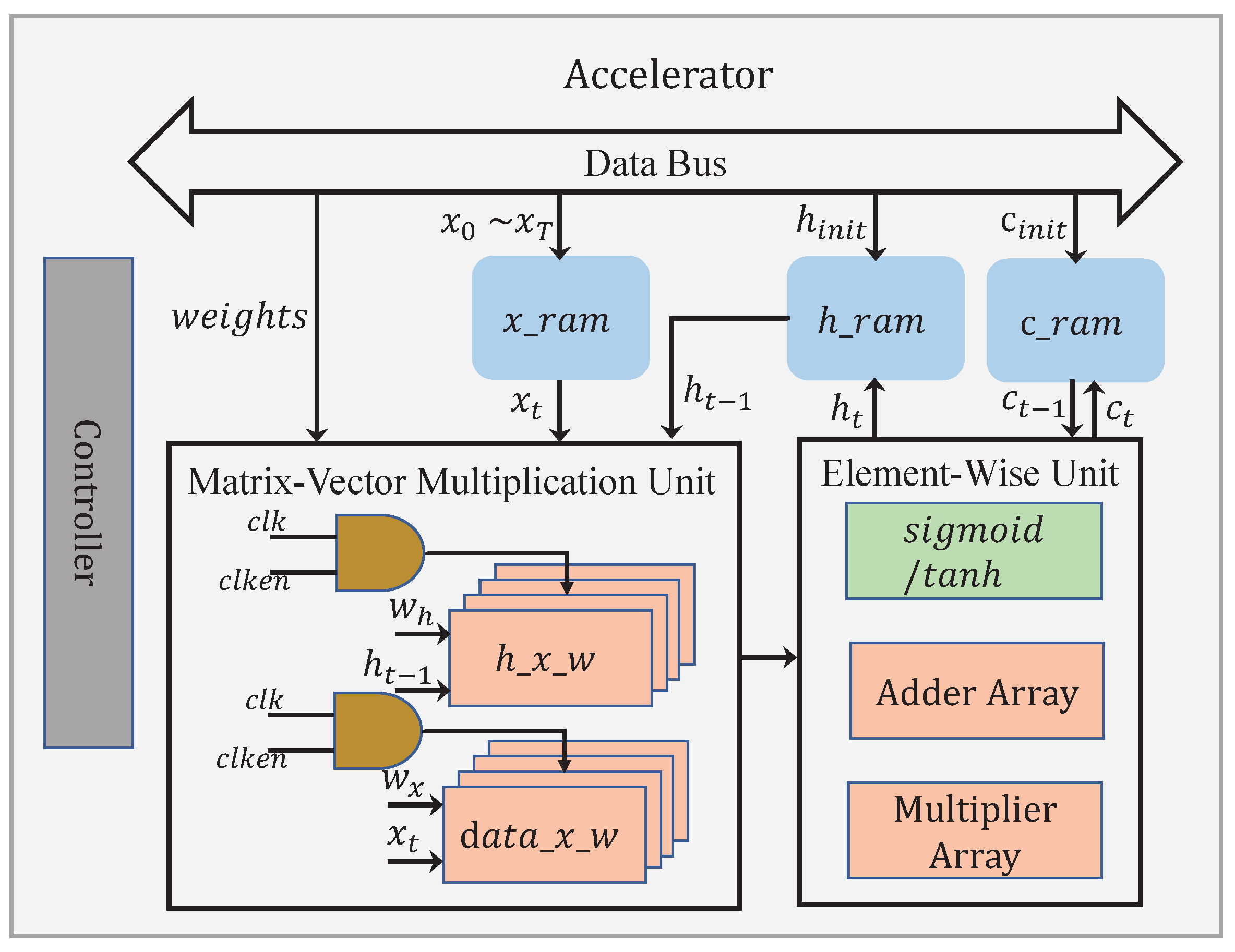
An architecture diagram for the proposed accelerator is shown in Figure 10. The accelerator has two main functional blocks, namely the matrix–vector multiplication unit and the element-wise unit, containing all the basic operations required by the LSTM. The matrix–vector multiplication unit is primarily responsible for the computations regarding ${\mathit{w}}_{*x}{\mathit{x}}_t$ and ${\mathit{w}}_{*h}{\mathit{h}}_{t-1}$ defined in Equations (1)–(4), where $*ϵ\{c,i,o,f\}$. As ${\mathit{w}}_{*x}ϵ{\mathbb{R}}^{m\times n}$ and ${\mathit{w}}_{*h}ϵ{\mathbb{R}}^{m\times m}$ are usually differing in dimension, the run times required to complete these two categories of multiplications are different. By exploiting the waiting intervals for the sake of energy saving, our architecture has two separate modules, i.e., $h\_x\_w$ and $data\_x\_w$, dedicated to accomplishing ${\mathit{w}}_{*x}{\mathit{x}}_t$ and ${\mathit{w}}_{*h}{\mathit{h}}_{t-1}$, respectively. When $m>n$, ${\mathit{x}}_t$ will be read from $x\_ram$ at a later time, in a way to align the finishing time for both matrix–vector multiplications. During the time before the next ${\mathit{x}}_t$ is read from $x\_ram$, the module $data\_x\_w$ is idle, with its clock disabled. When $n>m$, it should be the other way around. This time, reading ${\mathit{h}}_{t-1}$ from $h\_ram$ is being delayed until a later time, in the meantime setting the module $h\_x\_w$ at idle. By doing so, a big chunk of the total dynamic power consumption can be effectively cut off. For example, in a typical word sequence generation case, the difference between m (e.g., 27) and n (e.g., 256 or 512) could be quite large, benefiting the energy savings to a large extent. Note that the element-wise unit performs the element-wise addition, the element-wise multiplication, and the activation function.

Figure 10. The overall architecture of the proposed accelerator.

5.2. Matrix–Vector Multiplication

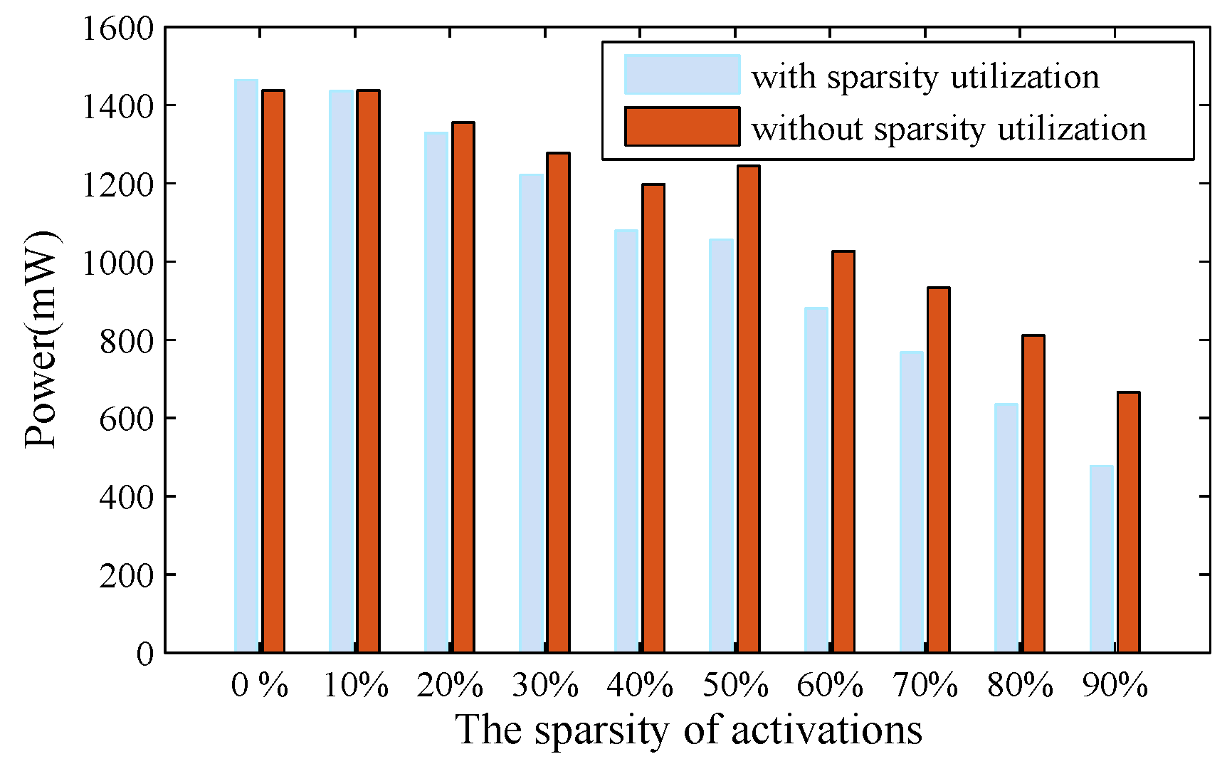
All the matrix–vector multiplications are regarded as the most computationally intensive during the LSTM inference. Therefore, an effort is directed towards possible reductions in such operations, by tapping into the enhanced sparsity in the weight, the activation, and the product after the compression. However, solutions to a complete treatment were seldom discussed in the prior works.

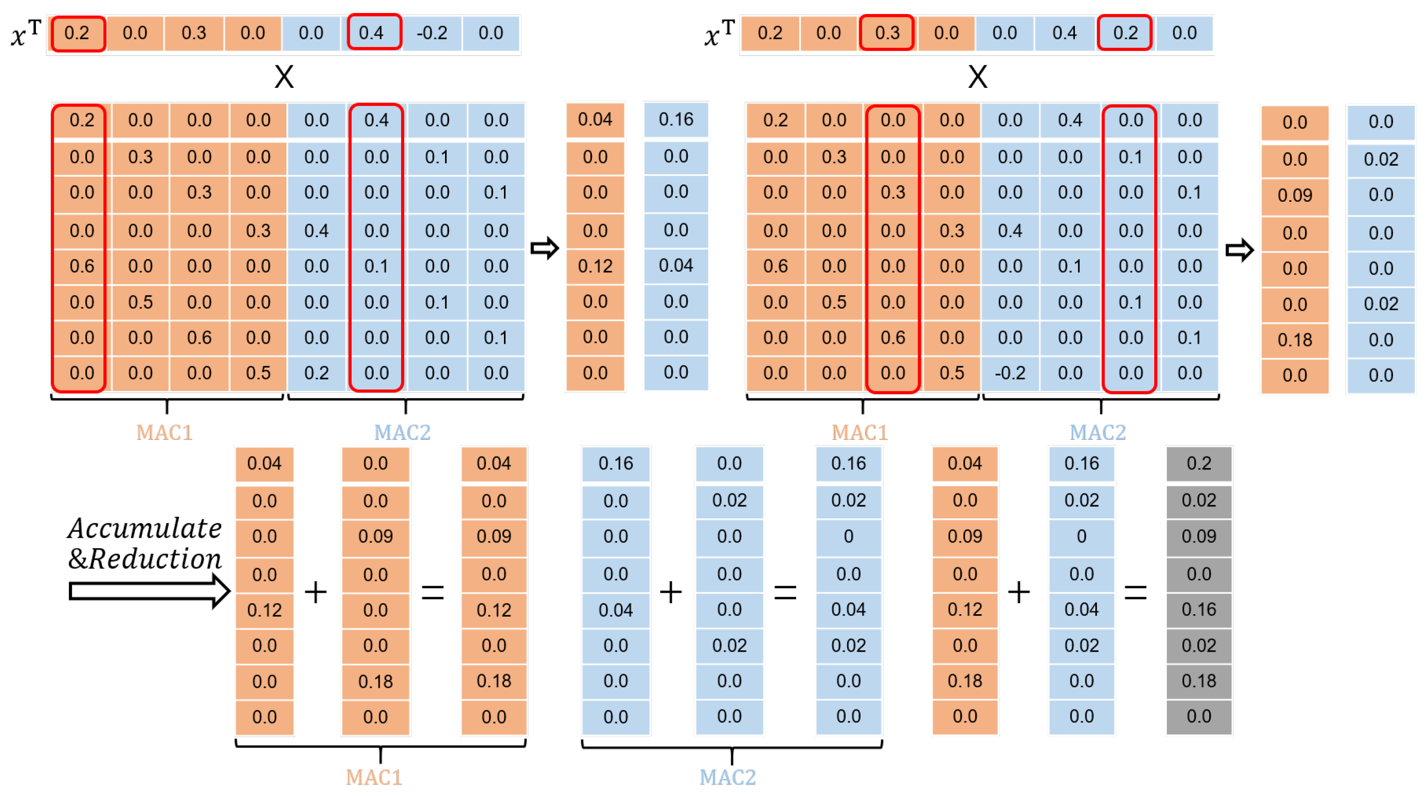
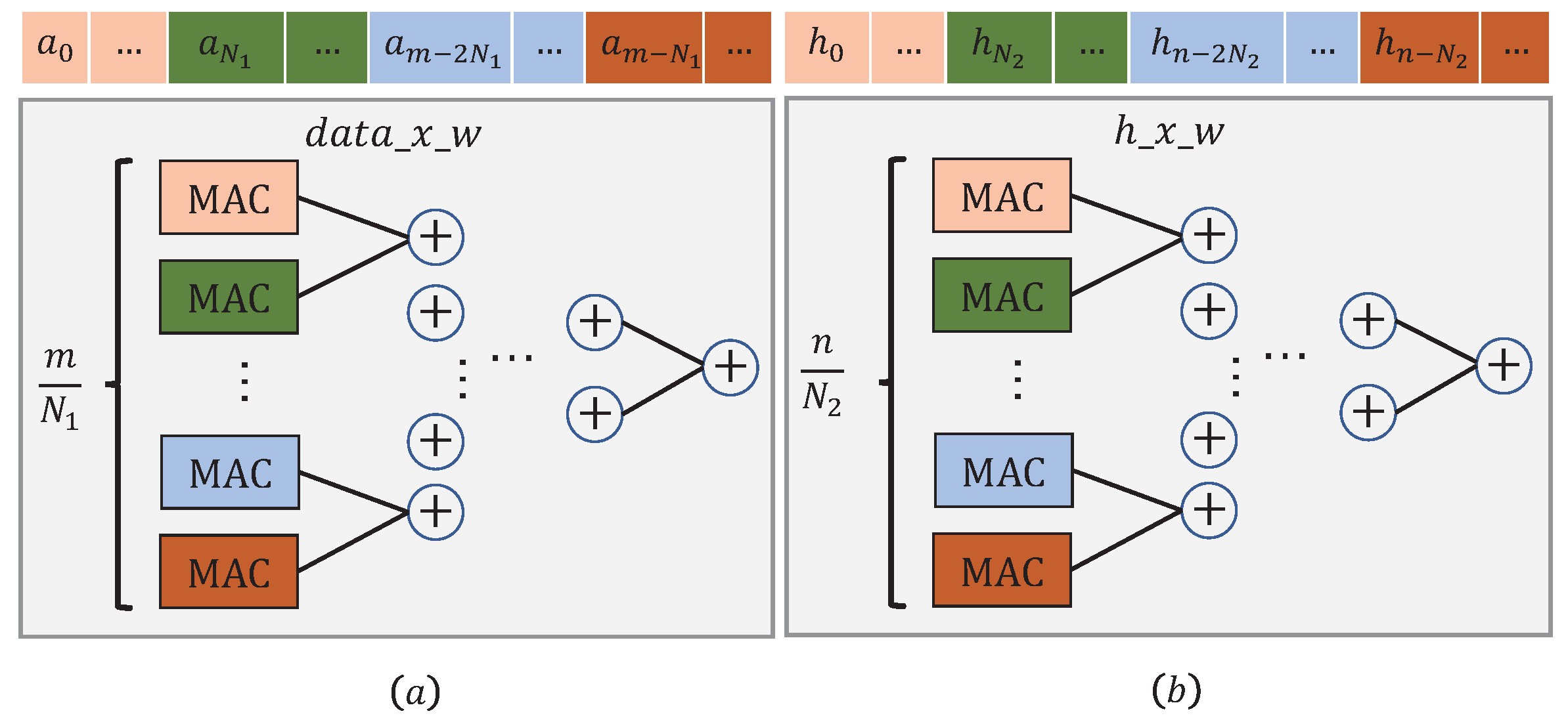
As for the activation, the accelerator has been designed to calculate the matrix–vector multiplications in a column-wise fashion, as depicted in Figure 11. As long as an activation $x_i$ is zero, the subsequent multiplications involving $x_i$ and ${\mathit{w}}_{:,i}$ will be bypassed. Here, ${\mathit{w}}_{:,i}$ represents all the weights from a corresponding column. Figure 12 illustrates the processing flow executed in module $data\_x\_w$. Along the way, m activations are being fed into $\frac{m}{N_1}$$MAC$ over $N_1$ clock cycles.

Figure 11. A column-wise processing procedure.

Figure 12. The processing flow of (a) Module $data\_x\_w$; (b) Module $h\_x\_w$.

Note that the MAC (Multiply and accumulate) unit marked in a color should coordinate those data slices marked with the same color. A similar procedure can also be applied to the module $h\_x\_w$.

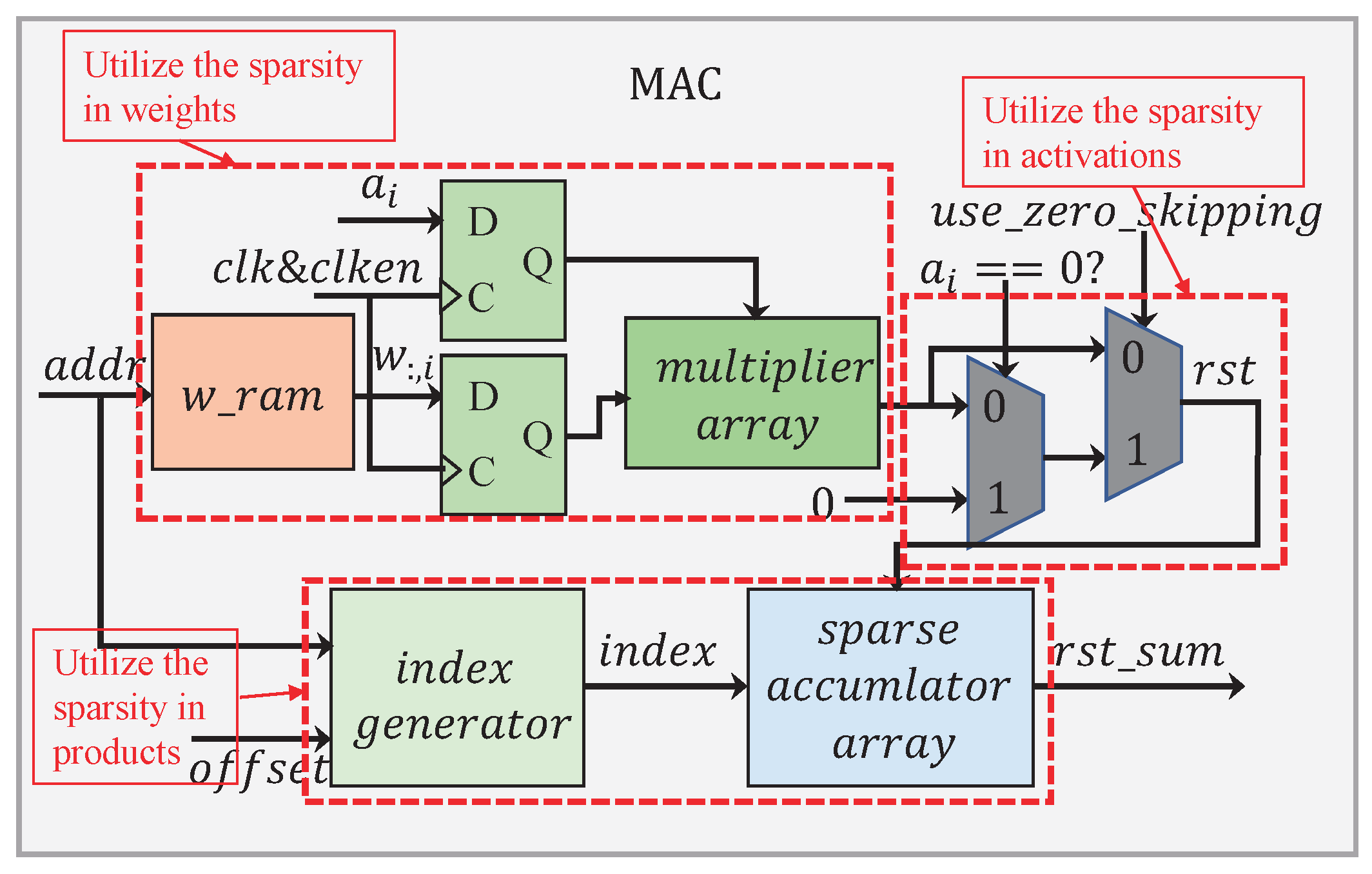
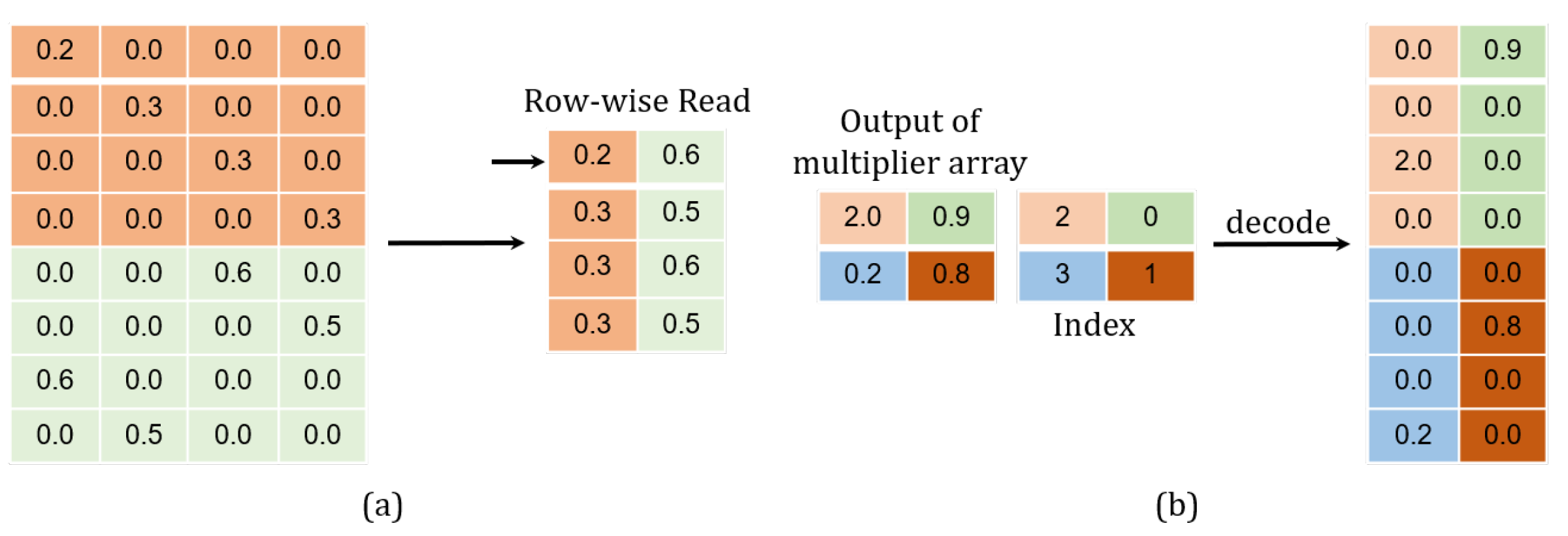
The MAC submodule has a processing flow as given in Figure 13. In order to reduce the memory footprint and lessen the multiplication operation, we developed a memory-accessing strategy by catering fully for the weight sparsity. As illustrated in Figure 14a, only non-zero weights at the same column in the matrix are stored along a single row in the memory, facilitating for them to be read once a clock cycle.

Figure 13. The processing flow of Module multiply and accumulate (MAC).

Figure 14. Process involving (a) data allocation into a weight memory; (b) data decoding into a recovered form.

In Figure 13, there are two 2:1 multiplexers that have been employed to dynamically configure the circuit according to the sparsity in the activation. When $a_i=0$, the first multiplexer selects zero as its output. At the same time, the clocking to those weight and activation registers is disabled. As a result, all the operations have been shut down in the multiplier array. Apparently, this allows for a great deal of power-saving, considering the activation being highly sparse. When $a_i\ne 0$, the result calculated from the multiplier array will pass straight through the first multiplexer. The second multiplexer is used to switch over between the zero-skipping and the non-zero-skipping modes, simply by controlling the signal $use\_zero\_skipping$, in a way to further cutting down the power consumption.

The sparsity in the product should also be taken into account. In order to have only the non-zero products sent for accumulation, their positions in the matrix need to be recorded. As long as either the multiplier or the multiplicand is zero, their product must be zero. In a way, the positions regarding these non-zero products are directly related to the corresponding non-zero weights. According to (7), the coordinates for the non-zero values in a weight matrix should observe the following relations:

$$\begin{array}{cc}\hfill & (offset+c)modp=d\hfill \\ \hfill ⟹& (offset+(imodp\left)\right)modp=jmodp\hfill \\ \hfill ⟹& \left(imodp\right)modp=jmodp-offsetmodp\hfill \\ \hfill ⟹& \left(imodp\right)=jmodp-offsetmodp\hfill \end{array}$$

(17)

In (17), the term $imodp$ calculates the longitude coordinate for all the non-zero weights in a relevant sub-matrix. Since the non-zero values belonging to the same column in the weight matrix are stored along a specific row in the memory $w\_ram$, j is then regarded as this row’s address ($w\_addr$). As for the offset, it can be decided just by a calculation of $\lfloor j/p\rfloor$, considering that $(\lfloor i/p\rfloor \times p)modp=0$. The module $indexgenerator$ takes such a differentiation route to determine all the locations regarding the non-zero products, e.g.,

$$\begin{array}{cc}\hfill index& =imodp\hfill \\ \hfill & =w\_addrmodp-(\lfloor w\_addr/p\rfloor )modp\hfill \end{array}$$

(18)

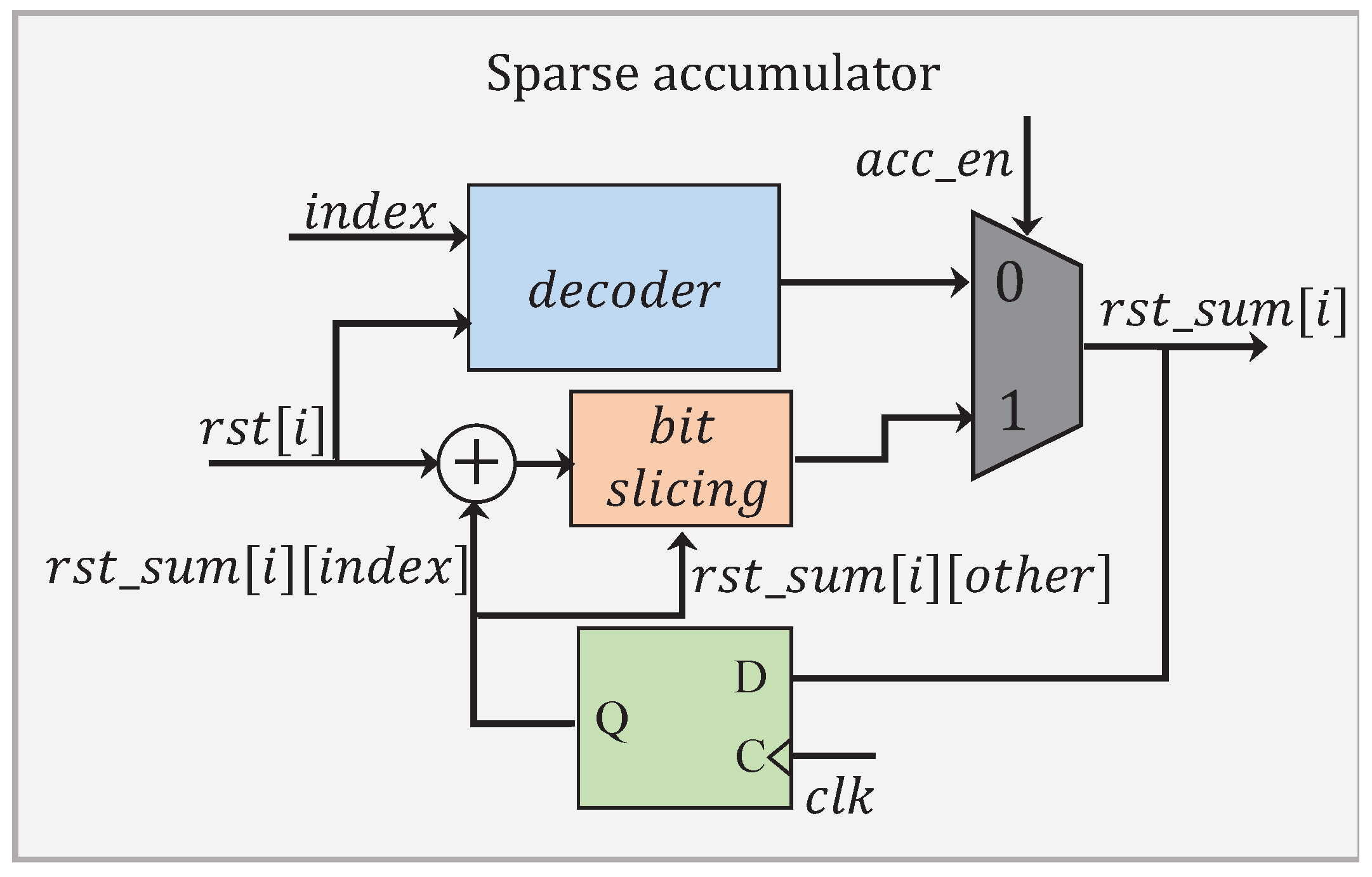
The module $Sparseaccumulator$ has a processing flow as depicted in Figure 15. When an accumulation is not required, the signal $acc\_en$ is set to 0. This allows for performing only the decoding operation, which has been illustrated in Figure 14b. The non-zero product $rst\left[i\right]$ is decoded in a format of $\{\overbrace{0\dots 0},\overbrace{0\dots 0},\dots ,\overbrace{rst\left[i\right]},\dots \}$. A total of p accumulated results are individually concatenated into $kp$ bits in the representation. When the accumulation is required, the signal $acc\_en$ is set to 1. Instead of performing all the p additions, only those additions involving $rst\left[i\right]$ and the corresponding contents in $rst\_sum\left[i\right]$ are processed. The intermediate results obtained are later stitched up with the others in $rst\_sum\left[i\right]$ to complete a full accumulation.

Figure 15. Block diagram of the sparsity-aware accumulator.

5.3. Operations Reduction Analysis

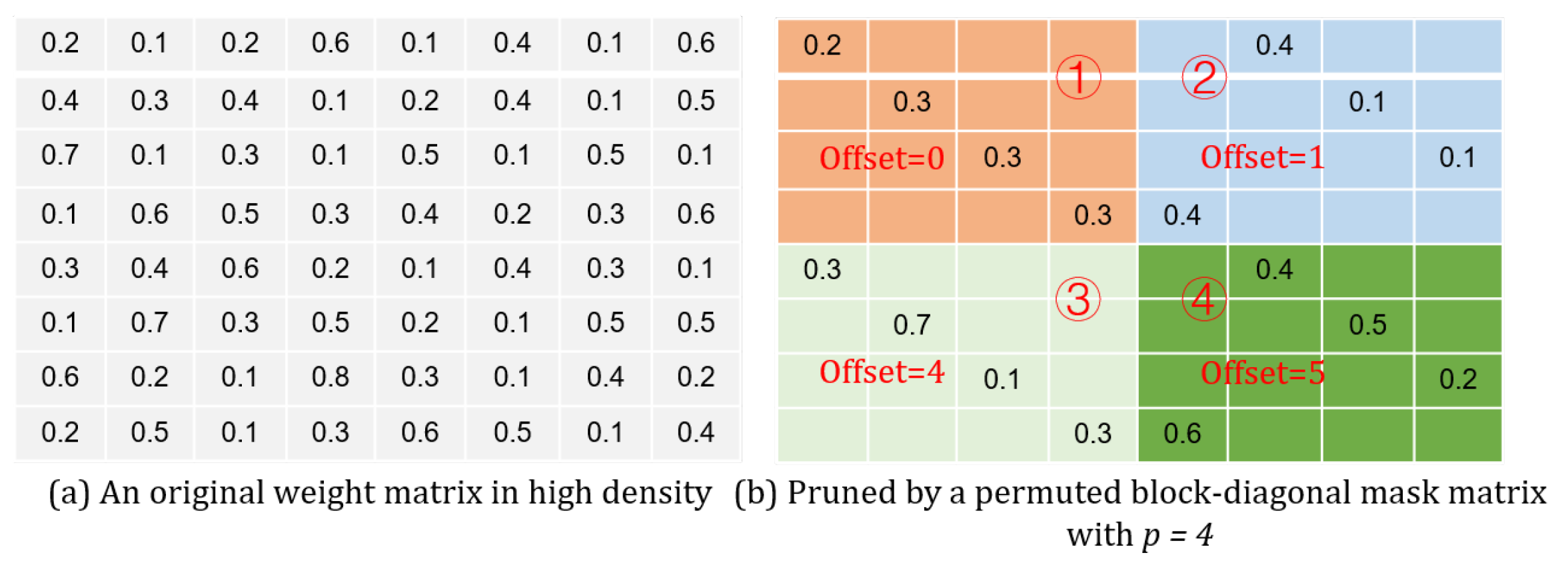
A theoretical analysis has been carried out on the reduced operation effect brought by our proposed design approach. For a weight matrix $\mathit{w}ϵ{\mathbb{R}}^{m\times n}$, it is pruned individually by $\frac{m}{p}\times \frac{n}{p}$ mask matrices in p-by-p dimensions. Hence, the ratio in terms of the multiplication reduction by treating the weight sparsity can be estimated as follows:

$$\begin{array}{cc}\hfill R_w& =\frac{\frac{m}{p}\times \frac{n}{p}\times p}{m\times n}\hfill \\ \hfill & =\frac{1}{p}\hfill \end{array}$$

(19)

Furthermore, suppose the non-zero activation ratio is $S_a$. In addition, all the weights take part in the multiplication have been pruned. Then, the multiplication reduction ratio due to attending the sparsity in the activation can also be estimated by:

$$R_a=\frac{1}{p}\times S_a$$

(20)

In terms of the product, the sparsity-aware processing can just lead to reducing the number of additions—in the case where the model is being pruned through the permuted block diagonal mask matrices, and the matrix–vector multiplication is being executed in a column-wise way (see Figure 11). In each column, there are $1\times \frac{m}{p}$ non-zero products. Thus, the number of the additions reduced, as a result from the product sparsity exploitation, can be calculated according to the following:

$$\begin{array}{cc}\hfill N_p& =S_a\times n\times (m-\frac{m}{p})\hfill \\ \hfill & =S_a\times n\times (p-1)\times \frac{m}{p}\hfill \end{array}$$

(21)

6. Experimental Results and Comparisons

Experiments are performed to evaluate the characteristics regarding our PermLSTM accelerator design. The performance results are further compared with some other state-of-the-art LSTM accelerators.

6.1. Experimental Setup

In our experiments, the Arria 10 (10AX115U4F45I3SG) FPGA (Intel, Santa Clara, CA, USA) is chosen to serve as a testing vehicle. The design coded in Verilog HDL is synthesized in the Quartus II 15.0 environment, operating at a frequency of 150 MHz. The Quartus PowerPlay (a dedicated Power Analyzer tool) is used to estimate post-placement power consumption of the device. The following operational conditions are assumed, i.e., (1) 25 °C ambient temperature; (2) 12.5% toggle rate for the I/O signals; (3) the real-time toggle rate applied to the core signals; (4) 0.5 static probability in BRAMs.

6.2. Breakdown of the Energy- and Resource-Saving Rates

The characteristics in terms of energy and resource saving vary with the weight/activation/product sparsity, which are measured and discussed. An original matrix–vector multiplication of ${\mathit{w}}_h{\mathit{h}}^{\mathit{T}}$ is referred to as a benchmark, where ${\mathit{w}}_hϵ{\mathbb{R}}^{120\times 120}$ and ${\mathit{h}}^{\mathit{T}}ϵ{\mathbb{R}}^{1\times 120}$. The number of MACs in module $h\_x\_w$ is set to 15, which implies that each MAC should perform 15 multiply-accumulate operations concurrently. The power dissipation and the resource utilization are examined on the following conditions: (1) none of the sparsity is considered (the baseline); (2) only the weight sparsity is considered; (3) both the weight and the activation sparsity are considered; (4) all of the sparsities involving the weight, the activation and the product are considered. The measurement results are presented in Table 4.

Table 4. The breakdown of both energy and resources saved by utilizing three types of sparsity.

The Sparsity of Activations	50%	Clock Frequency	150 MHz
The sparsity of weights	The sparsity of activations	The sparsity of products	Power (mW)	Logic utilization	Registers	DSP Blocks
✗	✗	✗	1941.72	21,036 (5%)	37,947	900
✓	✗	✗	1223.53	31,803 (8%)	34,747	225
✓	✓	✗	1035.26	31,803 (8%)	34,747	225
✓	✓	✓	871.63	23,182 (6%)	34,760	225

In the experiments, $m,n$, and p take the values of 120, 120, and 4, respectively. According to (19), the weight-sparsity related multiplication reduction rate ($R_w$) is 0.25 (1/4), which means 75% of the operations have now been cut out. Hence, the number of the DSP Blocks needed can be drastically reduced from 900 to 225. This gives rise to an effective power reduction by 718 mW.

Assume the sparsity ratio regarding the activation ($S_a$) be 50%. According to (20), the activation-sparsity related multiplication reduction rate ($R_a$) is 0.125 (1/8). This further reduces the multiplication runs. As a result, the power consumption is once again decreased by 188 mW.

In addition, assume the sparsity for the product to be the same as the weight. According to (21), the number of the reduced additions ($N_p$) is 5400. Obviously, this comprehensive weight/ activation/product sparsity-aware design delivers the lowest power consumption (871.63 mW) and the least resource utilization (minimum physical footprint in terms of logic fabrics and DSP blocks) by a remarkably large margin.

6.3. Influence by Different Levels of the Sparsity in Activation

As the weight sparsity is decided after the training, the activation sparsity is changing in real-time, which would influence how the power saving is estimated. Through varying the activation sparsity level from 0% to 90%, the power dissipations are measured in two conditions, i.e., with or without the activation sparsity undertaken in place. The results are shown in Figure 16. Seen as a general trend, the power is rapidly decreasing with the activation sparsity going up regardless. However, the advantage gap in favor of sparsity treatment against non-sparsity treatment becomes wider at high activation sparsity than at low activation sparsity. For an activation sparsity less than 10%, the power dissipations exhibited in both cases are almost leveled.

Figure 16. Power consumption vs. different levels of the sparsity in the activation.

6.4. Comparison with State-of-the-Art LSTM Accelerators

The following design parameters have been specified in our implementation: (1) the rank for the block-diagonal matrix is 4; (2) the bit-width for the weight is 4; (3) the bit-width for the activation is 7. Furthermore, there are 200 hidden nodes. Then, 25 $MACs$ in module $h\_x\_w$ are employed, with each $MAC$ performing 25 multiply-accumulate operations concurrently. Table 5 lists a statistic of the resources allocated in our design, based on the Vivado post-fitting reports. Because the low bit-width multipliers can be implemented with LUTs, no DSP blocks are required.

Table 5. The resource utilization of the PermLSTM accelerator.

ALMs	Registers
257,871 (60%)	351,258
BRAM (bits)	DSP
178,400	0

For the performance, we compared the proposed LSTM accelerator with five state-of-the-art LSTM accelerators, i.e., BBS [17], FINN-L [38], BRDS [18], DeltaRNN [39], and E-LSTM [40], all based on FPGAs. The results have been summarized in Table 6. To be fair, we choose the data of FINN-L with the bit-width setting being 4-4-4 (see note 1 in Table 6).

Table 6. Comparison with Other FPGA-Based Long Short-Term Memory (LSTM) Accelerators.

	BBS [17]	FINN-L [38]	BRDS [18]
Compression Approach	Bank-balanced Pruning	TLQ	Row-balanced Pruning
Platform	Arria 10	XCZU7EV	XCKU9P
Bit-width ${}^1$	16-16-16	4-4-4	16-16-16
Frequency (MHZ)	200	266	200
Throughput (GOPS, sparse)	304.1	1825	200
Throughput (GOPS, dense)	2432.8	1825	1600
Power ${}^2$ (W)	19.1	–	9.0
Efficiency (GOPS/W)	127.4	–	177.8
	Delta-RNN [39]	E-LSTM [40]	Ours
Compression Approach	Delta Network Algorithm	Top-K Pruning&Mixed Quantization	Permuted Block Diagonal Matrices&NLQ
Platform	XC7Z100	Arria 10	Arria 10
Bit-width ${}^1$	16-16-16	8-8-8	4-8-8
Frequency (MHZ)	125	200	150
Throughput (GOPS, sparse)	192	282.2	2220
Throughput (GOPS, dense)	1198	176.4	3345
Power ${}^2$ (W)	7.3	15.9	5.7
Efficiency (GOPS/W)	164.1	17.7	389.5

${}^1$ Consistent with the quantization level given in FINN-L, with the three numbers representing the bit-widths of weights, input activations and output activations respectively. ${}^2$ Measured power dissipation (not estimated).

Thanks to the coordinated simplification approach towards network compression, the proposed LSTM accelerator design achieves a throughput of 2.22 TOPS and an energy efficiency of 389.5 GOPS/W. Such processing performance demonstrates the $1.22\times$∼$10.49\times$ increase in throughput and the $2.19\times$∼$24.4\times$ improvement in energy efficiency, in comparison to some other state-of-the-art works.

7. Conclusions

In this paper, we presented a novel pruning and quantization approach. By using the permuted block mask matrices to prune model, we addressed the problem of structural irregularity and large indexing overhead. By normalizing the operands locally prior to the quantization, the problem of vanishing gradient is alleviated. Tapping into the high sparsity created by the proposed compression approach, an energy-efficient accelerator architecture called PermLSTM has been designed. In addition, based on our analysis on the quantization error effect regarding the participating operands on the activation function, the piecewise linear approximation is applied and tailored to match the activation bit-width selected after quantization. The design has been implemented on Arria-10 FPGA. According to the experimental results, PermLSTM achieves a throughput of 2.22 TOPS and an energy efficiency of 389.5 GOPS/W, demonstrating a superior processing performance in comparison to other prior works.