Verification in Relevant Environment of a Physics-Based Synthetic Sensor for Flow Angle Estimation ^†

Abstract

In the area of synthetic sensors for flow angle estimation, the present work aims to describe the verification in a relevant environment of a physics-based approach using a dedicated technological demonstrator. The flow angle synthetic solution is based on a model-free, or physics-based, scheme and, therefore, it is applicable to any flying body. The demonstrator also encompasses physical sensors that provide all the necessary inputs to the synthetic sensors to estimate the angle-of-attack and the angle-of-sideslip. The uncertainty budgets of the physical sensors are evaluated to corrupt the flight simulator data with the aim of reproducing a realistic scenario to verify the synthetic sensors. The proposed approach for the flow angle estimation is suitable for modern and future aircraft, such as drones and urban mobility air vehicles. The results presented in this work show that the proposed approach can be effective in relevant scenarios even though some limitations can arise.

1. Introduction

Following the recent aircraft crashes that occurred with the Boeing 737-MAX, the European Union Aviation Safety Agency (EASA) has become open to the use of synthetic sensors to estimate the flow angles [1]. The objective is to improve the reliability of redundant flow angle measurements, even using soft techniques starting with modern aircraft. To accommodate future applications of alternative solutions for flow angle estimations, a working group is defining the new standard AS7984 “Minimum Performance Standards, for Angle of Attack (AoA) and Angle of Sideslip (AoS)” to cover the various sensor technologies used to measure flow angles [2].

The flow angle synthetic sensor provides the same measurements as an equivalent physical sensor but without the use of dedicated equipment for this purpose. Generally speaking, a synthetic sensor, in fact, merges flight data already available on board in order to provide an additional measurement of one or more flight parameters. Therefore, a synthetic sensor can be used in replacement or combined with a conventional (physical) sensor with clear benefits from the point of view of: (i) reduction of weights and volumes; (ii) energy efficiency; (iii) dissimilarity with respect to conventional solutions.

In the field of synthetic sensors, different categories and examples are available in the literature [3,4,5,6], whereas the MIDAS project’s output [7] aims to be certified. The majority of the synthetic sensors developed so far, including those of the MIDAS project, suffer from common issues: (i) they can only be used on the aircraft where calibrated; (ii) they should be tuned on the aircraft’s current configuration and flight conditions; (iii) they require a tuning phase based on flight data.

State-of-the-art air data sensors are typically probes and vanes protruding externally from the aircraft fuselage, able to provide a direct measurement of air data, mainly pressures, flow angles and air temperature. In the era of digital avionics, synthetic sensors can be added to physical (or mechanical) sensors in order to analytically increase the system redundancy [8,9]. Another potential application is to use synthetic sensors to monitor physical sensors and to accommodate possible failures [10,11]. The concurrent use of dissimilar sources of the same air data (physical and synthetic ones) can be beneficial for solving some issues related to common failure modes or incorrect failure diagnosis of modern air data systems [12,13,14]. Moreover, synthetic sensors can be used to overcome some issues towards certification related to next generation air vehicles, for example, unmanned aerial vehicles (UAVs) [15] and urban air mobility (UAM) aircraft [16] without any limitations to the application domain [17,18,19].

Some examples of the synthetic estimation of flow angles can be found in [20,21,22,23,24,25,26]. Model-based (e.g., Kalman filter) and data-driven (e.g., neural networks) are the approaches commonly used to estimate flow angles that are designed ad hoc for a particular aircraft and, therefore, they are affected by changes of configuration and flight regime. A model-free, or physics-based, nonlinear scheme, named ASSE—Angle-of-Attack and Sideslip Estimator—is proposed in [27] and aims to have a general validity and to therefore be independent from the aircraft application or flight regime.

In fact, ASSE deals with an analytical approach that is able to provide a generic synthetic sensor for flow angle estimation applicable to any flying body independently from the flight configuration and without the need to be calibrated. ASSE is based on an analytical formulation (or scheme) that, compared to the state-of-the-art, is better suited to be certified for civil aviation. The present work is part of the project SAIFE [28]—Synthetic Air Data and Inertial Reference System—where a demonstrator of the ASSE technology is designed and manufactured to verify the Technology Readiness Level (TRL) 5. The technological demonstrator is based on “all-in-one” air data and inertial system (commonly known as ADAHRS) able to provide multiple information to pilots or to automatic control systems, partially based on synthetic sensors that are used for flow angle estimation. The proposed approach for flow angle estimation does not require dedicated physical sensors but at the same time guarantees, under recognisable circumstances, the same reliability of flow angle vanes (or probes) in order to optimise the efficiency of on board avionics for both modern and future aircraft.

The main aim of the current work, as part of the project SAIFE, is to verify the TRL 5 of the ASSE technology. For this goal, a technological demonstrator is conceived and fully characterised in order to evaluate the uncertainty budgets related to all physical sensors feeding the synthetic sensors. Therefore, results of the present work describe the flow angle estimation performance of the ASSE scheme in a relevant simulated scenario. It is worth underlining that results presented in this work have a general validity as the flight simulator is only used to generate coherent and, hence, the proposed ASSE scheme can be applied to any flying body to estimate the flow angles. Moreover, the technological demonstrator is equipped with all necessary components to be ready for flight tests for future validation in real environments.

The SAIFE project’s demonstrator concept is introduced in Section 2 with a focus on the architecture and its physical sensors. The ASSE scheme is briefly presented in Section 3 in order to highlight the necessary inputs and to discuss some practical limitations emerged from the present work. The characterisation tests of the physical sensors and the consequent sensor’s noisy models are defined in Section 4, whereas the approach for TRL 5 verification and results are presented in Section 5 before concluding the work.

2. The ASSE Technological Demonstrator Concept

The ASSE technological demonstrator is depicted in Figure 1a along with: (a) external power supply to be connected both to the aircraft power bus or to domestic plug; (b) global navigation satellite system (GNSS) antenna; (c) magnetometer antenna; (d) pitot boom with AoA and AoS vanes. The ASSE demonstrator, encompassing both air data, inertial and heading reference systems (ADAHRS) is able to provide the following direct measurements:

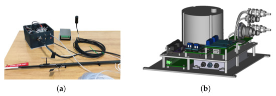
Figure 1. ASSE demonstrator design. (a) A view of the ASSE technological demonstrator developed under the SAIFE project, (b) Arrangement design. Courtesy of SELT Aerospace & Defence.

• from the Air data System (ADS):

  1.

  Dynamic pressure $q_c$ (or, as alternative, total pressure);

  2.

  Absolute pressure $p_{\infty }$;

  3.

  Ambient temperature T;

  4.

  Angle-of-attack AoA (as a reference value);

  5.

  Angle-of-sideslip AoS (as a reference value);

• from the Attitude and Heading Reference System (AHRS):

  6.

  3-axis angular rates;

  7.

  3-axis linear accelerations;

  8.

  3-axis magnetometer;

  9.

  2-axis inclinometer;

  10.

  GNSS position and velocity;

The output rate is 100 $\mathrm{Hz}$. In order to provide ADS outputs, the demonstrator shall be interfaced with at least an external probe (e.g., a Pitot probe) able to measure the dynamic and absolute pressure and a temperature probe (e.g., outside ambient temperature, OAT). Whereas, for AHRS outputs, common equipment (described in Section 2.3) is used that can be installed inside the fuselage. From the aforementioned direct measurements, several parameters can be calculated, such as the attitude angles, the heading and the true airspeed, whereas, the flow angles are estimated using the ASSE technology (described in Section 3.1). Therefore, the only probes protruding externally from the fuselage are related to pressure and temperature measurements.

2.1. State-of-the-Art of Air Data System Sensors

As far as low speed (Mach number below $0.3$) air vehicles are concerned, the air temperature is commonly measured with OAT, which is able to directly measure the ambient static temperature with a sensing element exposed to the external airflow.

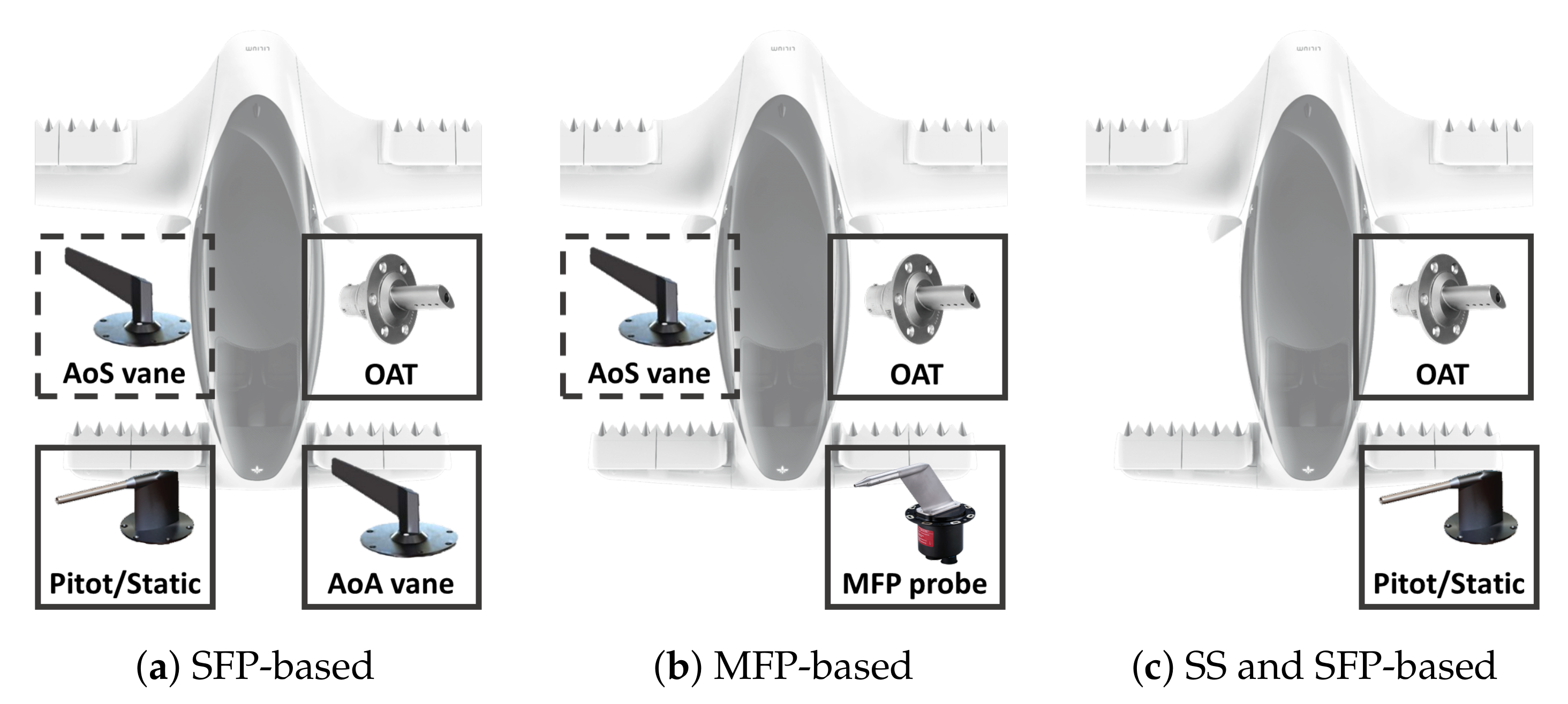
As far as the pressures are concerned, two probe technologies are available: (1) the single-function probes; and (2) the multi-function probes. The conventional pressure probes (or single-function probes, SFP) considered here are total tubes (for the total pressure measurement), Pitot-static (or simply Pitot) probes (for static and total pressure measurements) or static ports (for static pressure measurement). In the majority of the examples, the conventional pressure probes are not equipped with pressure transducers, so that they have to be connected pneumatically to dedicated air data modules (ADMs), an air data computer (ADC) or a vehicle management computer (VMC). On the other side, a multi-function probe (MFP) is a probe with enhanced capabilities able to provide at least two pressure measurements and one flow angle measurement. The pressure measurements are usually related to static and total pressures, whereas the flow angle is referred to a local flow angle and only a combination of at least two MFPs can provide both AoA and AoS calculation. In the MFP category, the optical air data sensors could be considered even though there is no certified product at the moment because some issues still remain to be solved [29], for example, turbulence, vortex and wind gusts can affect the accuracy.

Considering the state-of-the-art of the current technologies, three realistic architectures for air data and inertial reference system are compared in Figure 2. An ADS based on SFP leads to a high number of LRUs to be installed protruding outside from the A/C fuselage as schematically represented in Figure 2a with a consequent increase of weight and power. However, the SFPs are mature and available worldwide. Whereas, MFPs are available only from three manufacturers [30] but it can assure a reduced number of LRUs and the absence of pneumatic tubes as represented in Figure 2b. In Figure 2c, a possible ADS based on flow angle synthetic sensors is presented. Along with the chance to use SFP probes, the other main advantages of an ADS based on flow angle synthetic sensors are: (i) a reduced number of LRUs with a consequent reduction of weights and volumes; (ii) no power required for anti-icing systems improving the overall ADS energy efficiency; (iii) improved safety due to dissimilarity with respect to other conventional flow angle vanes/probes.

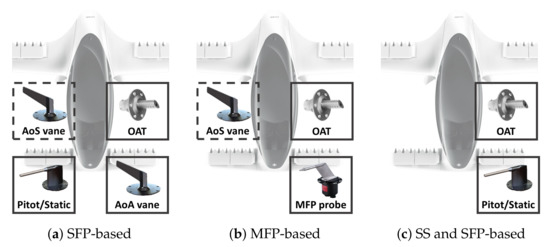
Figure 2. Generic three realistic simplex air data sensing architectures able to provide a complete set of air data. The dashed lines of AoS sensors indicate that they could not be mandatory.

It is worth underlining that the realistic sensing architectures presented in Figure 2 can provide the same air dataset in a simplex configuration. As some flight parameters can be safety critical; according to safety studies, a suitable redundancy should be assured, for example, for airspeed and AoA. Therefore, some external probes should be duplicated, or even triplicated, to satisfy the safety requirements. Although the system redundancy on board large airplanes does not represent an issue, the same can lead to some obstacles to UAVs or UAM vehicles due to the reduced fuselage surface suitable for air data probe installation. Therefore, the solutions based on fewer external LRUs can be more attractive for those categories.

2.2. Demonstrator’s Architecture

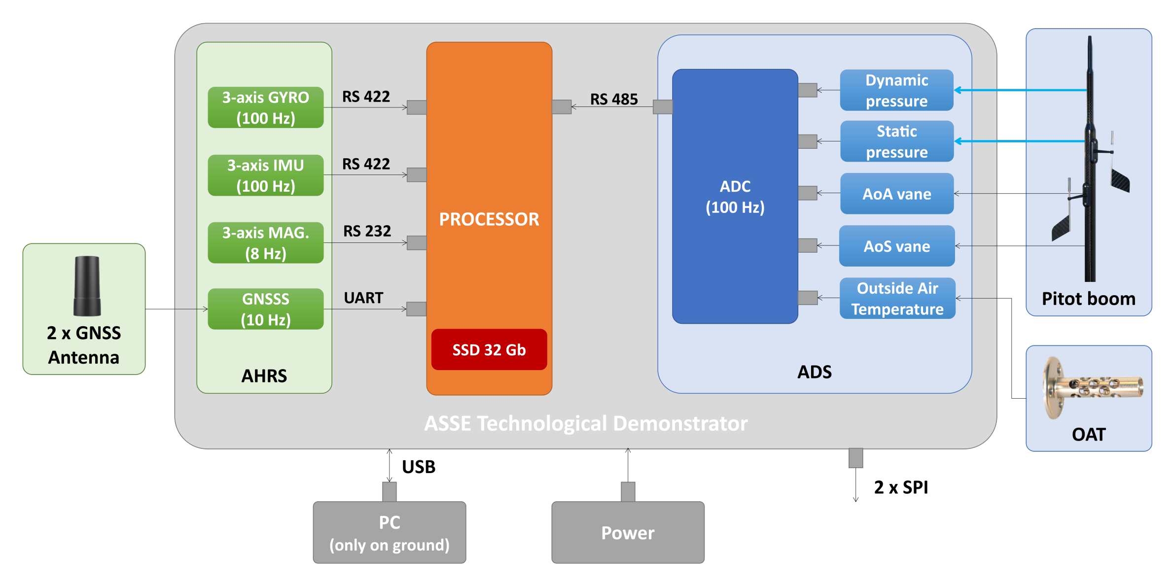
The ASSE demonstrator is based on the TEENSY $4.1$ board that is able to manage digital and analog interfaces as described in Figure 3. It is designed to be interfaced with AHRS sensors (described in Section 2.3), air data transducers (described in Section 2.4) and a ground computer. It is worth highlighting that the ADS is also equipped with AoA and AoS common vanes because during the demonstration they are used as reference values during actual flight tests.

Figure 3. The architecture of the ASSE technological demonstrator. The black arrows represent data bus connections, the blue arrows represent pneumatic connections.

The AHRS and ADC are installed in a single unit (or LRU) as described in Figure 1b. The reason behind a two-layer board is to keep the center of gravity as close as possible to the gyroscope and the accelerometers.

The aircraft heading and attitudes during dynamic manoeuvres are evaluated using ad hoc Kalman filters exploiting available data from the gyroscope, accelerometers, magnetometers and GNSS. For the scope of the present work, the attitude angles are unnecessary and they are replaced with inclinometer information for integration tests.

2.3. Attitude, Heading and Reference Sub-System

The ASSE demonstrator is based on fibre optic gyroscope (FOG), a solid state accelerometer unit, a GNSS receiver and a 3-axis magnetometer as represented in Figure 3.

2.4. Air Data Sub-System

The ASSE demonstrator also includes an air data sub-system comprising an ADC with pressure transducers, calibrated interfaces for OAT and flow angle vanes. The ADC is calibrated to work in the airspeed range [0 kn, 174 kn] in the altitude range [−1800 ft, 35,000 ft].

3. Nonlinear ASSE Scheme

In this section, the ASSE scheme is presented in order to give some crucial information about the proposed technology.

Two reference frames are considered: the inertial reference frame ${\mathcal{F}}_I=\left\{X_I,Y_I,Z_I\right\}$ and the body reference frame ${\mathcal{F}}_B=\left\{X_B,Y_B,Z_B\right\}$ as described in Figure 4. The vector transformation from the inertial reference frame ${\mathcal{F}}_I$ to the body frame ${\mathcal{F}}_B$ is obtained considering the ordered sequence 3-2-1 of Euler angles: heading, elevation and bank angles. As the vector subscript denotes the reference frame where the vector is represented, the relationship between the inertial velocity ${\mathbf{v}}_I$, the relative velocity ${\mathbf{v}}_B$ and the wind velocity ${\mathbf{w}}_I$ can be written as:

$${\mathbf{v}}_I={\mathbf{C}}_{B2I}{\mathbf{v}}_B+{\mathbf{w}}_I,$$

(1)

where ${\mathbf{C}}_{B2I}$ is the direction-cosine matrix to calculate vector components in the inertial reference frame from the body reference frame [31]. It is worth recalling that the inverse transformation is ${\mathbf{C}}_{I2B}={\mathbf{C}}_{B2I}^T$, that is, the direction-cosine matrix to calculate vector components in the body reference frame from the inertial reference frame [31]. The relative velocity ${\mathbf{v}}_B$ can be expressed as function of its module and flow angles, $\alpha$ and $\beta$, as

$$\begin{array}{cc}\hfill {\mathbf{v}}_B& =V_{\infty }{\widehat{\mathit{i}}}_{WB}=V_{\infty }\left(cos\beta cos\alpha {\widehat{\mathit{i}}}_B+sin\beta {\widehat{\mathit{j}}}_B+cos\beta sin\alpha {\widehat{\mathit{k}}}_B\right),\hfill \end{array}$$

(2)

where $V_{\infty }$ is the magnitude of the relative velocity vector, or true airspeed (TAS), ${\widehat{\mathit{i}}}_B$, ${\widehat{\mathit{j}}}_B$ and ${\widehat{\mathit{k}}}_B$ are the three unit vectors defining the body reference axes and ${\widehat{\mathit{i}}}_{WB}$ is the unit vector of ${\mathbf{v}}_B$ depending only on $\alpha$ and $\beta$.

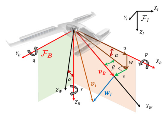
Figure 4. Representation of inertial and body reference frames with positive flow angles ($\alpha$, $\beta$), linear relative velocities (u, v, w), angular rates (p, q, r) and the velocity triangle between inertial velocity ${\mathbf{v}}_I$, the relative velocity ${\mathbf{v}}_B$ and the wind velocity ${\mathbf{w}}_I$.

Recalling that ${\mathsf{\Omega }}_B$ is defined as the body angular rate matrix [32], the coordinate acceleration ${\mathbf{a}}_B$ can be written as:

$$\begin{array}{c}\hfill {\mathbf{a}}_B={\mathbf{C}}_{I2B}{\mathbf{a}}_I={\dot{\mathbf{v}}}_B+{\mathsf{\Omega }}_B{\mathbf{v}}_B+{\mathbf{C}}_{I2B}{\dot{\mathbf{w}}}_I=a_{X_B}{\widehat{\mathit{i}}}_B+a_{Y_B}{\widehat{\mathit{j}}}_B+a_{Z_B}{\widehat{\mathit{k}}}_B.\end{array}$$

(3)

3.1. The ASSE Synopsis

As known, the time-derivative of the relative velocity’s magnitude can be expressed as:

$${\dot{V}}_{\infty }=\frac{{\mathbf{v}}_B^T{\dot{\mathbf{v}}}_B}{V_{\infty }}\Rightarrow {\dot{V}}_{\infty }{V}_{\infty }={\mathbf{v}}_B^T\left({\mathbf{a}}_B-{\mathbf{C}}_{I2B}{\dot{\mathbf{w}}}_I\right),$$

(4)

where all terms are measured at the same time instant. Moreover, the relative velocity vector ${\mathbf{v}}_B$ at time t can be expressed starting from ${\mathbf{v}}_B$ at a generic time $\tau$, with $t\ge \tau$, as

$${\mathbf{v}}_B\left(t\right)={\mathbf{v}}_B\left(\tau \right)+{\int }_{\tau }^t{\dot{\mathbf{v}}}_B\left(\mathcal{T}\right)d\mathcal{T}.$$

(5)

Henceforth, in order to ease the notation, the independent variable of the integrand function is omitted and the time of the measurement is reported as subscript. For example, the relative velocity evaluated at time $\tau$ is denoted as ${\mathbf{v}}_{B,\tau }$.

Recalling Equation (3), Equation (5) can be rewritten as:

$${\mathbf{v}}_{B,t}={\mathbf{v}}_{B,\tau }+{\int }_{\tau }^t\left({\mathbf{a}}_B-{\mathsf{\Omega }}_B{\mathbf{v}}_B-{\mathbf{C}}_{I2B}{\dot{\mathbf{w}}}_I\right)d\mathcal{T}$$

(6)

and

$${\mathbf{v}}_{B,\tau }={\mathbf{v}}_{B,t}-{\int }_{\tau }^t{\mathbf{a}}_{B}d\mathcal{T}+{\int }_{\tau }^t{\mathsf{\Omega }}_B{\mathbf{v}}_{B}d\mathcal{T}+{\int }_{\tau }^t{\mathbf{C}}_{I2B}{\dot{\mathbf{w}}}_{I}d\mathcal{T}.$$

(7)

Replacing ${\mathbf{v}}_{B,\tau }$ with Equation (7), Equation (4) can be written at time $\tau$ as:

$$V_{\infty ,\tau }{\dot{V}}_{\infty ,\tau }={\left[{\mathbf{v}}_{B,t}+{\int }_{\tau }^t{\mathsf{\Omega }}_B{\mathbf{v}}_{B}d\mathcal{T}\right]}^T{\left({\mathbf{a}}_B-{\mathbf{C}}_{I2B}{\dot{\mathbf{w}}}_I\right)}_{\tau },$$

(8)

where all terms depending on ${\mathbf{v}}_B$, and hence on the flow angles, are collected on the right hand side.

The ASSE scheme based on the zero-order approximation [27] assumes that the integral term ${\int }_{\tau }^t{\mathsf{\Omega }}_B{\mathbf{v}}_{B}d\mathcal{T}$ of Equation (8) is constant in the generic time interval $\left[\tau ,t\right]$, therefore

$${\int }_{\tau }^t{\mathsf{\Omega }}_B{\mathbf{v}}_{B}d\mathcal{T}={\left({\mathsf{\Omega }}_B{\mathbf{v}}_B\right)}_t\Delta t,$$

(9)

where $\Delta t=t-\tau$. Considering the latter expression, Equation (8) can be rewritten as:

$$\begin{array}{cc}\hfill V_{\infty ,\tau }{\dot{V}}_{\infty ,\tau }& +{\left[{\int }_{\tau }^t{\mathbf{a}}_{B}d\mathcal{T}-{\int }_{\tau }^t{\mathbf{C}}_{I2B}{\dot{\mathbf{w}}}_{I}d\mathcal{T}\right]}^T{\left({\mathbf{a}}_B-{\dot{\mathbf{w}}}_B{\mathbf{C}}_{I2B}{\dot{\mathbf{w}}}_I\right)}_{\tau }=\hfill \\ \hfill =& V_{\infty ,t}{\widehat{\mathbf{i}}}_{WB,t}^T\left(\mathbf{I}-{\mathsf{\Omega }}_{B,t}\Delta t\right){\left({\mathbf{a}}_B-{\mathbf{C}}_{I2B}{\dot{\mathbf{w}}}_I\right)}_{\tau }.\hfill \end{array}$$

(10)

Equation (10) is denoted in [27] as the basic expression of the zero-order ASSE scheme referred to the generic time $\tau$ where the flow angles, $\alpha \left(t\right)$ and $\beta \left(t\right)$, are the only unknowns and all other terms are supposed to be measured. For the latter reason, the unknown variables are always referred to as current time t, henceforth, the flow angles are represented without subscripts related to time.

Considering the previous notations, Equation (10) can be presented as:

$$\begin{array}{cc}\hfill n_{\tau }& ={\widehat{\mathbf{i}}}_{WB,t}^T{\mathbf{m}}_{\tau },\hfill \end{array}$$

(11)

where

$$n_{\tau }=V_{\infty ,\tau }{\dot{V}}_{\infty ,\tau }+{\left[{\int }_{\tau }^t{\mathbf{a}}_{B}d\mathcal{T}-{\int }_{\tau }^t{\mathbf{C}}_{I2B}\dot{\mathbf{w}}d\mathcal{T}\right]}^T{\left({\mathbf{a}}_B-{\mathbf{C}}_{I2B}\dot{\mathbf{w}}\right)}_{\tau }$$

(12)

and

$${\mathbf{m}}_{\tau }=V_{\infty ,t}\left(\mathbf{I}-{\mathsf{\Omega }}_{B,t}\Delta t\right){\left({\mathbf{a}}_B-{\mathbf{C}}_{I2B}{\dot{\mathbf{w}}}_I\right)}_{\tau }=h_{\tau }{\widehat{\mathit{i}}}_B+l_{\tau }{\widehat{\mathit{j}}}_B+m_{\tau }{\widehat{\mathit{k}}}_B.$$

(13)

It is worth underlining that, in Equation (13), all parameters are referred to as time $\tau$, whereas the true airspeed $V_{\infty ,t}$ is always referred to as time t and, hence, AoA and AoS as well. Rewriting Equation (11) back in time starting from t to n-th generic ${\tau }_i$ with $i\in \left[0,1,\dots ,n\right]$ where ${\tau }_0\equiv t$ and AoA and AoS are always referred to at the same time t. Therefore, the following system of $n+1$ nonlinear equations, or ASSE scheme, is obtained:

$$\left\{\begin{array}{c}{n}_t={\widehat{\mathbf{i}}}_{WB,t}^T{\mathbf{m}}_t\hfill \\ n_{{\tau }_1}={\widehat{\mathbf{i}}}_{WB,t}^T{\mathbf{m}}_{{\tau }_1}\hfill \\ ⋮\hfill \\ n_{{\tau }_n}={\widehat{\mathbf{i}}}_{WB,t}^T{\mathbf{m}}_{{\tau }_n},\hfill \end{array}\right.$$

(14)

where the AoA and AoS at time t are assumed to be the only unknowns, the wind acceleration $\dot{\mathbf{w}}$ is considered to be negligible in the time interval and all other parameters can be measured. Therefore, the flow angle estimation based on the ASSE scheme requires direct measurements of: (1) TAS; (2) body angular rates p, q and r and (3) coordinate acceleration vector ${\mathbf{a}}_B$. It is worth highlighting that the AHRS does not measure the coordinate acceleration vector but it can be calculated from the inertial acceleration directly measured by the AHRS in addition to the aircraft attitudes (or Euler angles).

Equation (14) is the generic form of the proposed zero-order ASSE scheme based on $n+1$ equations. In this work, an expansion in the past is considered (${\tau }_{i+1}<{\tau }_i$). The most suitable solver can be adopted to solve the system of Equation (14) for AoA and AoS estimation.

3.2. Practical Implementation

As discussed in [33], solving the ASSE nonlinear scheme can be challenging dealing with real signals that are affected by uncertainties mainly related to random noise, bias, drift of the sensors. In fact, more robust solvers can be considered to solve the ASSE scheme that are more tolerant to the input noise. In this work, the nonlinear ASSE scheme [34] with 200 time steps (or equations) is adopted to validate the ASSE demonstrator. The number of equations indicates that the ASSE scheme is applied considering a 2 $\mathrm{s}$ time observation. The latter choice is based on the experience gained with the present project to improve the ASSE performance characteristics in the presence of noisy input with respect to results presented in [33]. In this work, the system of nonlinear equations is solved using an iterative method based on the Levenberg–Marquardt algorithm [35]. The first guess in iteration methods is crucial but it is hardly realistic considering a reliable first guess in practical applications; therefore, the proposed scheme is applied, adopting null values as the initial condition.

As known from [27], the ASSE scheme can be applied only during dynamic flight conditions. Moreover, from [34], the linear formulation can lead to understanding where ASSE can be applied or not. In order to introduce the reliability criteria, the linearised ASSE scheme is discussed. Considering Taylor series expansions of trigonometric functions, the versor of Equation (2) can be approximated at first order (i.e., $cos\left(x\right)\approx 1$ and $sin\left(x\right)\approx x$) as:

$${\widehat{\mathbf{i}}}_{WB,t}\approx {\tilde{\mathbf{i}}}_{WB,t}={\left[1,\beta ,\alpha \right]}^T.$$

(15)

Therefore, writing Equation (14) for time t and a generic previous time $\tau$ (with $\tau <t$), the following system of two linear equations is obtained:

$$\left\{\begin{array}{c}{n}_t={\widehat{\mathbf{i}}}_{WB,t}^T{\mathbf{m}}_t\approx h_t+l_t{\beta }_{lin}+m_t{\alpha }_{lin}\hfill \\ n_{\tau }={\widehat{\mathbf{i}}}_{WB,t}^T{\mathbf{m}}_{\tau }\approx {\tilde{\mathbf{i}}}_{WB,t}^T{\mathbf{m}}_{\tau }=h_{\tau }+l_{\tau }{\beta }_{lin}+m_{\tau }{\alpha }_{lin}.\hfill \end{array}\right.$$

(16)

Moreover, considering that the wind acceleration vector $\dot{\mathbf{w}}$ is negligible, for example, if the two observed time steps are sufficiently close to consider the wind vector constant in the time interval $\left[\tau ,t\right]$, Equation (16) can be rewritten as:

$$\left\{\begin{array}{c}{\alpha }_{lin,\dot{\mathbf{w}}\approx 0}=\frac{a_{Y,t}\left({\dot{V}}_{\infty ,\tau }-a_{X,\tau }\right)-a_{Y,\tau }\left({\dot{V}}_{\infty ,t}-a_{X,t}\right)}{D_{\dot{\mathbf{w}}\approx 0}}\hfill \\ {\beta }_{lin,\dot{\mathbf{w}}\approx 0}=\frac{a_{Z,\tau }\left({\dot{V}}_{\infty ,t}-a_{X,t}\right)-a_{Z,t}\left({\dot{V}}_{\infty ,\tau }-a_{X,\tau }\right)}{D_{\dot{\mathbf{w}}\approx 0}},\hfill \end{array}\right.$$

(17)

where

$$D_{\dot{\mathbf{w}}\approx 0}=l_{t,\dot{\mathbf{w}}\approx 0}{m}_{\tau ,\dot{\mathbf{w}}\approx 0}-m_{t,\dot{\mathbf{w}}\approx 0}{l}_{\tau ,\dot{\mathbf{w}}\approx 0}$$

(18)

is the determinant of the system evaluated with negligible wind accelerations and it shall be nonzero to guarantee the existence of the closed-form solution.

In order to evaluate possible flight conditions leading to a null determinant, it is worth noting that the determinant $D_{\dot{\mathbf{w}}\approx 0}$ does not depend on the time derivative of the airspeed but only on the true airspeed, body accelerations and angular rates; the latter weighted by the chosen time interval $\Delta t$. In fact, when the time interval tends to zero, the $\mathbf{m}$ vector of Equation (13) can be approximated as ${\mathbf{m}}_{\tau }={\left[h_{\tau },l_{\tau },m_{\tau }\right]}^T\approx V_{\infty ,t}{\left[a_{X,\tau },a_{Y,\tau },a_{Z,\tau }\right]}^T$ yielding to the following determinant approximation:

$$D_{\dot{\mathbf{w}}\approx 0,\Delta t\to 0}=V_{\infty ,t}^2\left(a_{Y,t}{a}_{Z,\tau }-a_{Z,t}{a}_{Y,\tau }\right).$$

(19)

Along with the existence condition discussion presented in [34], from Equation (19) it emerges that a null simplified determinant could lead to very large errors. Therefore, some thresholds are defined according to a trial and error approach where the nonlinear ASSE scheme would lead to very large errors (larger than 5°). The proposed values can be possible values for real applications even though they should be verified in an extended flight envelope. In this work, the following thresholds are considered:

• vertical/lateral inertial acceleration:
  • $a_Z>a_{thr}=0.5 \mathrm{m} {\mathrm{s}}^{-2}$ for AoA estimation
  • $a_Y>a_{thr}=0.5 \mathrm{m} {\mathrm{s}}^{-2}$ for AoS estimation
• determinant of Equation (18): $\tilde{D}>D_{thr}=0.2 {\mathrm{m}}^4/{\mathrm{s}}^6$,

where the determinant $D_{\dot{\mathbf{w}}\approx 0}$ of Equation (18) is denoted henceforth as $\tilde{D}$ for simplicity of notation. The latter conditions are used to drive the integration tests of the demonstrator’s algorithms. In fact, even in the case of larger time intervals (i.e., $\Delta t>0$), if lateral or vertical inertial accelerations are very small (i.e., $a_Y\to 0$ or $a_Z\to 0$, respectively) the determinant tends to zero and the condition number will be very large leading to a very noise-sensitive scheme. It is worth underlining that, in this work, the thresholds do not influence the results because they are only applied after the ASSE solution is computed.

Moreover, considering that there are no metrological standards to evaluate the synthetic sensor performance [36], some criteria are defined to evaluate the flow angle estimation performed by the nonlinear ASSE scheme. In this work, the flow angle estimations are analysed using the mean, maximum, $1\sigma$ and $2\sigma$ errors. The latter choice, inspired by industrial experience, is useful for providing an overall overview of the flow angle estimation performances. In the present work, $1\sigma$ and $2\sigma$ intended the value such that the probability $Pr\left(-\sigma \le X\le \sigma \right) =68.3\%$ and $Pr\left(-2\sigma \le X\le 2\sigma \right) =95.4\%$ also in the case the error is not normally distributed. If the mean error can be easily removed from the synthetic sensor estimations, the maximum and the $2\sigma$ errors should be specified according to their operative scopes. In fact, if AoA and AoS are used for monitoring or displaying purposes, maximum absolute errors up to 5° could be accepted, whereas, for control and navigation applications the performance requirements could be more demanding. However, considering the stage of the present project, the following thresholds are considered in the current work:

• maximum absolute error <5°
• $2\sigma$ error <2°.

4. Characterisation of the ASSE Demonstrator’s Sensors

The section introduces the methods and results of the characterisation activities for the ASSE demonstrator’s sensors. Calculated uncertainties are used to corrupt simulated flight data with realistic errors that are added to reproduce a relevant testing scenario as defined in this section.

The three-axes gyroscope and the three-axes accelerometer are tested separately to verify their performances independently from manufacturer’s data sheets using a rotating platform to verify the angular rates, whereas tilting and sliding platforms are used to verify the linear acceleration performances. Once the AHRS sensors are installed in the ASSE demonstrator, the same characterisation tests are performed to verify possible misalignment issues. For the sake of clarity, the characterisation presented in this section is related to the technological demonstrator.

In more detail, three dedicated facilities are used to calibrate the inertial sensor at the best accuracy level. The fibre optic gyroscope (FOG) is calibrated against a rotating platform. The platform is based on a precision air-bearing table driven by a microstep motor. The platform is able to generate smooth and accurate rotation ranging from fractions of a degree per second to the full range of the device, which is greater than 400° s⁻¹.

The FOG is mounted in three orthogonal positions in order to calibrate the three axes and to check for the orthogonality of the measurement axis. The accuracy of the orthogonality is checked by a precision autocollimator and the accuracy of the rotating table is checked by comparison with the National Angle Standard (REAC) [37].

The accelerometers, or the inertial measurement unit (IMU), is calibrated for very low accelerations with a tilt table platform where the projection of the acceleration gravity vector parallel to the platform is used as a reference acceleration. The technique has been already used for the calibration of the accelerometers on board the ESA spacecrafts BepiColombo and JUICE with destinations of Mercury and Jupiter [38]. For higher accelerations, the device is calibrated using a facility built to the purpose making use of dynamic laser interferometry having an accuracy of at least 1 × 10⁻⁴ m s⁻². In this case, the accelerometers are also calibrated at the three orthogonal axes.

The ADS is stimulated using the pressure test bench. Thanks to suitable probe adapters, the air data probe is connected pneumatically to the pressure test bench that is able to generate both the static and the total pressures. Moreover, the pressure test bench is able to simulate both constant and dynamic flight conditions according to predefined steps that can be set by the user. The temperature sensor is connected and left to the ambient temperature.

4.1. Gyroscope

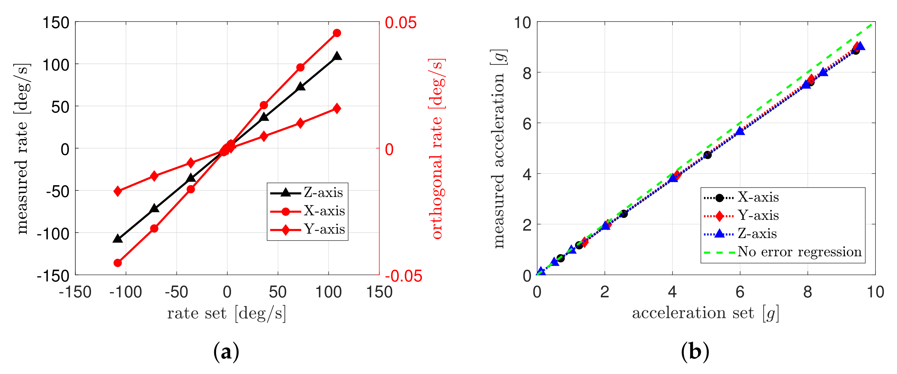
The FOG is tested to characterise the uncertainties on the measurement for several constant angular rates and periodic angular rates with several frequencies in order to evaluate both steady-state and dynamic errors and, hence, to evaluate the FOG’s expanded uncertainty. An example of the steady-state gyroscope measurements is represented in Figure 5a with respect to the reference values on the Z-axis. From the Figure 5a it is clear that at 0 $\mathrm{Hz}$, the gyroscope is characterised by a linear behaviour; in fact, the regression slope is $1.00$ and the $R^2=1.00$. Moreover, a cross-coupling between the three axes is visible even though it is less than 0.05%. Including dynamic analysis, the expanded uncertainty on the angular rates measured by the ASSE demonstrator is evaluated as Q(0.05,5 × 10⁻⁴ ν). The notation Q(0.05,5 × 10⁻⁴ ν) is intended to be the quadratic sum of two terms: the first is the constant, the second is proportional to the measured value $\nu$. For example, for 100° s⁻¹, the uncertainty is $U=\sqrt{0.{05}^2+{\left(100·5\times {10}^{-4}\right)}^2}=\sqrt{0.0025+0.0025}\approx 0.071° {\mathrm{s}}^{-1}$. If the error distribution is normal, the $U=2\sigma$. In this work, the latter assumption is adopted. Therefore, the single axis gyroscope measurements, p, q, r, are corrupted with a white noise whose $1\sigma$ depends on the measurement itself. For example, the pitch rate q is corrupted using a white noise with $1\sigma$ calculated as $q_{1\sigma }=\frac{1}{2}\sqrt{0.{05}^2+q^2{\left(5\times {10}^{-4}\right)}^2}$$° {\mathrm{s}}^{-1}$.

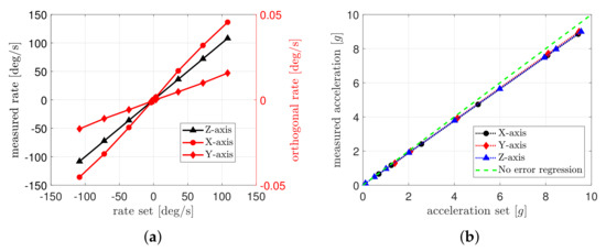
Figure 5. Example of AHRS data analysis. (a) Constant angular rate on the Z-axis, (b) Dynamic accelerations at 80 Hz.

4.2. Inertial Measurement Unit

The IMU is tested to characterise the uncertainties on the measurement for several constant accelerations and periodic accelerations with several frequencies in order to evaluate both steady-state and dynamic errors and, therefore, to evaluate the expanded uncertainty. An example of dynamic measurements with periodic reference accelerations at 80 $\mathrm{Hz}$ are represented in Figure 5b. From the Figure 5b it is clear that at 80 $\mathrm{Hz}$, the inertial measurement unit loses accuracy. In fact, even though the linearity is maintained, because with a linear regression $R^2=1.00$, the slope is $0.941$, whereas for very low frequencies (less than $5\mathrm{Hz}$) the regression slope is $1.00$ for each of the three axis. This particular behaviour is taken into account with a very large expanded uncertainty of $\mathrm{Q}(0.007,0.02 \nu )$ up to 10 g and up to 80 $\mathrm{Hz}$. It is worth underlying that for realistic aircraft applications, limiting the frequency to 10 $\mathrm{Hz}$ as discussed in Section 4.8, the expanded uncertainty can be recalculated as Q(0.007,1 × 10⁻³ ν). In this work, the largest values are considered for conservative reasons. The single axis acceleration measurements, $a_X$, $a_Y$, $a_Z$, are corrupted with a white noise whose $1\sigma$ depends on the measurements itself. For example, the longitudinal accelerations $a_X$ are corrupted using a white noise with $1\sigma$ calculated as $a_{X,1\sigma }=\frac{1}{2}\sqrt{0.{007}^2+a_X^{2}0.{02}^2}$ $\mathrm{m} {\mathrm{s}}^{-2}$.

4.3. Inclinometer

The two-axes inclinometer is tested to characterise the uncertainties on the measurement for several constant inclinations in order to evaluate the steady-state errors and, therefore, to evaluate its expanded uncertainty. As the inclinometer is only used for initialisation purposes, it is not considered in the uncertainty chain for the ASSE scheme. In fact, the attitude angles are calculated with a dedicated algorithm but they are not involved in the verification activities of the present work. However, the inclinometer is used to verify the ASSE algorithm during integration tests where the attitude angle is used to derive the inertial acceleration $\mathit{a}$ from the proper acceleration $\mathit{a}+\mathit{g}$ measured by the IMU, where the vector $\mathit{g}$ is the gravity vector. The measured expanded uncertainty is $\mathrm{Q}(0.2,0.01 \nu )$ in the range [−60°, 60°].

4.4. Calibrated Airspeed

Some airspeed profiles are simulated in terms of velocity and altitude using the pressure test bench. As said before, the pressure test bench has two independent pressure ports to provide both static and dynamic pressures. The air data probe is connected pneumatically to the pressure test bench using a suitable probe adapter. With the latter experimental setup, the air data test set is able to stimulate the ADC with predefined airspeed and pressure altitude according to a predefined rate that can be programmed by the user. Preliminarily, the ADC of the ASSE demonstrator is calibrated using reference values of airspeed generated using the pressure test bench.

The 2nd order calibration polynomial is derived fitting the error measured during the bench tests at ambient temperature as represented in Figure 6a. The residual maximum error after the calibration is about 0.05 m s⁻¹ as can be noted in Figure 6a.

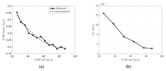
Figure 6. Calibrated airspeed analysis. (a) Measured and calibration of the IAS calculated by the ASSE demonstrator, (b) Noise on the CAS measurement.

A high-pass filter with 1 $\mathrm{Hz}$ cutoff frequency is used to evaluate the random noise on the CAS measurement. From Figure 6b, it is clear that the noise on the measurement of the CAS is less than 1.3 × 10⁻³ m s⁻¹.

The air data test set can maintain a constant value of airspeed with internal controllers with a total uncertainty of 0.26 m s⁻¹. This leads to the assumption that the CAS measurement uncertainty is dominated by unknown bias errors and less influenced by the random noise on the measurement. Therefore, the uncertainty of the CAS measurement is modelled as the sum of: (1) a bias not depending on the CAS itself calculated as the sum of the residual error after the calibration plus the contribution of the reference values generated; (2) white noise whose 1σ value is derived from the maximum of Figure 6b to be conservative. Therefore, in this work, the realistic CAS (or the CAS with uncertainties) is obtained using CAS_bias = 3.1 × 10⁻² m s⁻¹ and CAS_1σ = 1.3 × 10⁻³ m s⁻¹.

As far as the dynamic pressure error is concerned, the main uncertainty can be evaluated considering the sole ${\mathrm{CAS}}_{bias}$ as $q_{c,bias}=\sqrt{\frac{1}{2}{\rho }_{SL}\left|{\left(\mathrm{CAS}\pm CA{S}_{bias}\right)}^2-{\mathrm{CAS}}^2\right|}$, where ${\rho }_{SL}=1.225 \mathrm{k}\mathrm{g}/{\mathrm{m}}^3$.

4.5. Altitude

Some constant altitudes are simulated in terms of static pressure using the pressure test bench. As said before, using suitable probe adapters, the air data probe is connected pneumatically to the pressure test bench that is able to stimulate the ADC’s absolute pressure transducer. As a first step, the ADC of the ASSE demonstrator is calibrated using reference values of static pressure (or altitudes) generated using the pressure test bench.

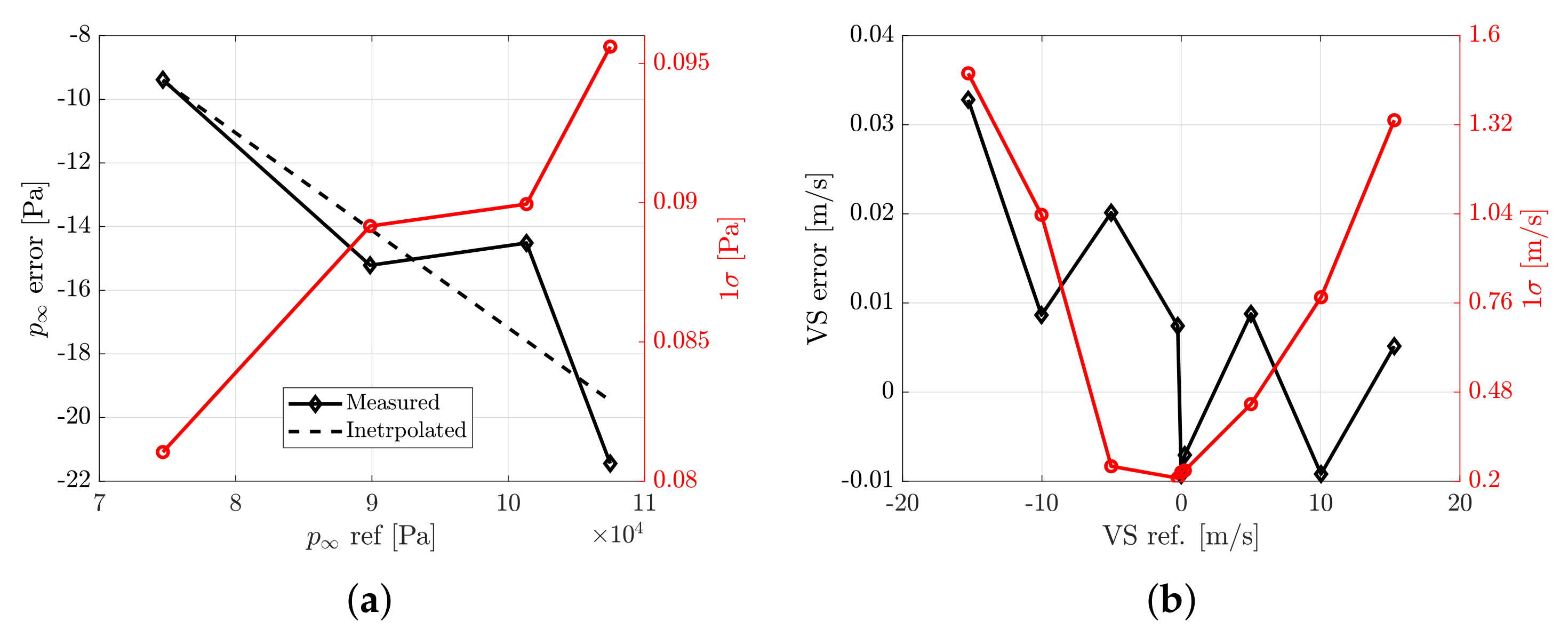
A linear regression is used to fit the error measured during the bench tests at ambient temperature as represented in Figure 7a. The residual maximum error after the calibration is about 3 $\mathrm{Pa}$, as can be seen from Figure 7a.

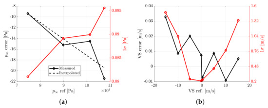
Figure 7. Altitude and vertical speed uncertainty analysis. (a) Static pressure, (b) Vertical speed.

Considering 30 $\mathrm{s}$ time windows, the random noise is allocated to the $1\sigma$ error of the measured static pressure. The noise on the measurement of the static pressure is less than $0.1$ $\mathrm{Pa}$ and it is practically constant if compared with the mean errors. For conservative reasons, the latter value is used in this work.

From the latter analysis, the static pressure measurement uncertainty is dominated by unknown bias errors and less influenced by the random noise of the measurement. Therefore, adopting the same model of the CAS presented in Section 4.4, the uncertainty on the static pressure measurement is modelled as the sum of a constant bias and white noise. Therefore, the uncertainty model of the static pressure is obtained using $p_{\infty ,bias}=3.0\mathrm{Pa}$ and $p_{\infty ,1\sigma }=0.1\mathrm{Pa}$. Applying the proposed static pressure error model in a realistic altitude range between $-500$ $\mathrm{m}$ and 3000 $\mathrm{m}$ for ultralight aircraft applications, the maximum uncertainty is enclosed in $\pm 3\mathrm{Pa}$ (or $\pm 0.36 \mathrm{m}$) as can be noted from Figure 7a. It is worth underlining that the latter result is related to the sole ASSE demonstrator without considering any position errors due to the aircraft installation.

4.6. Vertical Speed

In this section, the vertical speed uncertainty is evaluated even though it is not used in the ASSE scheme. In fact, it is reported here to provide some additional information of the ADC performance. Some constant vertical speeds are simulated in terms of static pressure using the pressure test bench connected to the ADC using suitable probe adapters. Results are presented in Figure 7b and it is clear that the VS uncertainty is dominated by the random noise. Therefore, the calculated expanded uncertainty for the vertical speed is $\mathrm{Q}(-0.00551,0.00518\nu )$.

4.7. True Airspeed

The same uncertainty model of the CAS can be applied to the TAS measurement with higher values due to uncertainty related to the temperature and pressure uncertainties. In fact, the error in terms of the TAS calculation can be estimated as:

$$\mathrm{TAS}=\sqrt{\frac{2\left(q_c\pm q_{c,bias}\right)R\left(T\pm \Delta T\right)}{p_{\infty }\pm p_{\infty ,bias}}}=V_{\infty }+{\mathrm{TAS}}_{bias},$$

(20)

where R = 287.06 J kg⁻¹ K⁻¹ is the air specific gas constant. The quantity ΔT = ±2.5 °C, whereas $q_{c,bias}$ and $p_{\infty ,bias}$ are the largest bias error calculated according to models presented in Section 4.4 and Section 4.5 respectively. Therefore, in this work, the resulting ${\mathrm{TAS}}_{bias}=\pm 0.47\mathrm{m} {\mathrm{s}}^{-1}$, whereas ${\mathrm{TAS}}_{1\sigma }={\mathrm{CAS}}_{1\sigma }$.

4.8. Time Derivative of the Airspeed

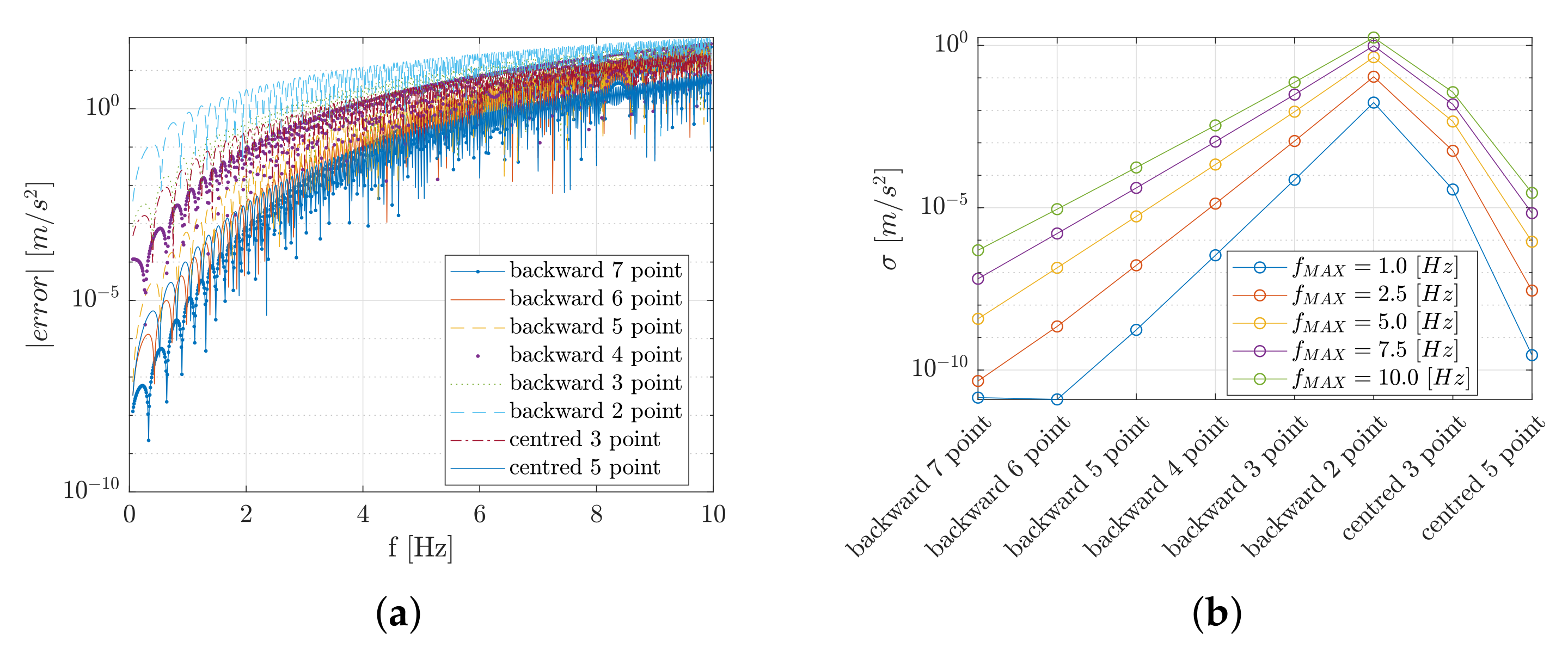
The airspeed time derivative is a crucial measurement for ASSE applications. As the direct measurement cannot be taken, several schemes [39] are considered in this work: (i) backward two point 1st order; (ii) backward three point 2nd order; (iii) backward four point 3rd order; (iv) backward five point 4th order; (v) backward six point 5th order; (vi) backward seven point 6th order; (vii) centred three point 2nd order; (iix) centred five point 4th order. The numerical derivative is denoted as $\tilde{\dot{y}}$. In order to evaluate the numerical estimation error at several frequency of several derivative schemes, a linear increasing frequency cosine function and its exact derivative are defined as

$$\begin{array}{cc}\hfill & y=cos2\pi ft\hfill \\ \hfill & \dot{y}=-4\pi f_{max}\frac{t}{t_{end}}sin2\pi ft,\hfill \end{array}$$

(21)

where $t\in \left[0,t_{end}\right]$ is the time in seconds and $f=f_{max}\frac{t}{t_{end}}$ is the increasing frequency and $f_{max}=10\mathrm{Hz}$ is the maximum frequency. The maximum frequency is chosen considering the target application of the ASSE demonstrator during flight trials. In fact, as an ultralight motorised aircraft is chosen for flight tests, the highest dynamic mode frequencies are not greater than 5 $\mathrm{Hz}$. The same can be applicable for UAV, UAM, general aviation and civil aircraft. Considering a constant sampling time, the absolute error $\left|\tilde{\dot{y}}-\dot{y}\right|$ is reported in Figure 8a as a function of the frequency for several schemes. It is clear that: (1) the lower the frequency, the lower the error; (2) the higher the scheme order, the lower the error. The same conclusions can be obtained from another analysis that are summarised in Figure 8b. In the latter analysis, only five frequencies are selected ( 1 $\mathrm{Hz}$, $2.5$ $\mathrm{Hz}$, 5 $\mathrm{Hz}$, $7.5$ $\mathrm{Hz}$ and 10 $\mathrm{Hz}$) and the $1\sigma$ error (i.e., $\tilde{\dot{y}}-\dot{y}$) is calculated over an entire period. As noted before, the 7-point backward scheme shows the best performance among the backward schemes with comparable performances to those achieved with the 5-point centred scheme.

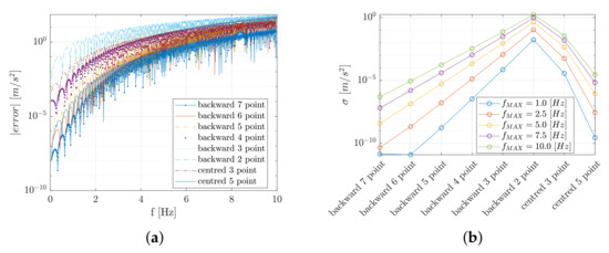
Figure 8. Error estimation of the numerical derivative estimation of Equation (21) at different frequencies. (a) Numerical derivative estimation at different frequencies, (b) $1\sigma$ error for different frequencies.

The $1\sigma$ error analysis reported in Figure 8b is very important to build the error model for the airspeed time derivative as shown at the end of the current section.

Although the best solution could be a centred derivative scheme, in this work, the backward schemes are preferred as the refresh rate of the estimated flow angles is considered aligned to all other parameters. Of course, other implementations with one or two step delays (i.e., 3-point and 5-point centred schemes respectively) can be accepted according to the specific final application (e.g., if it does not affect the control logics). However, the choice of the differential scheme is not made at the moment as the objective of the present analysis is to characterise the numerical derivative uncertainty.

The ASSE demonstrator’s sampling rate is not constant due to the hardware implementation of several devices with different output rate and computational load. In fact, the ASSE demonstrator sampling rate is 0.01 s ± 0.002 s as experienced in a log file record of more than 2 min.

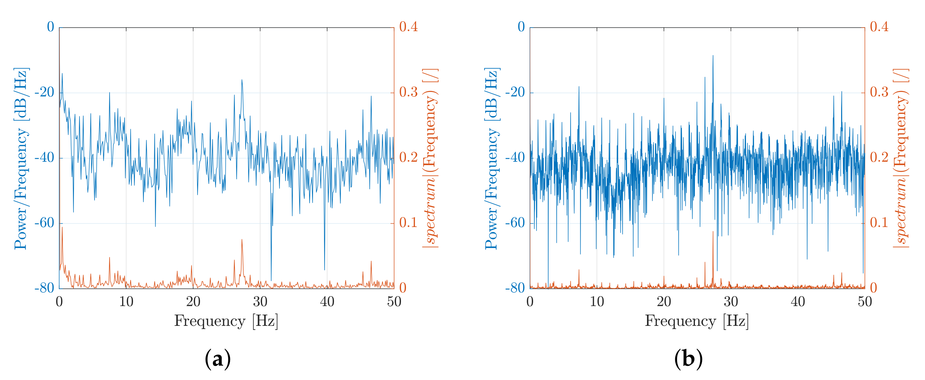
Using the pressure test set, constant airspeed rates are generated at a constant altitude in order to avoid interference of the total and static pressure controllers. However, from the frequency analysis of Figure 9a, it emerged that the positive airspeed rates are affected by the pressure test set’s controller (between $0.5$ $\mathrm{Hz}$ and 20 $\mathrm{Hz}$), whereas the negative rates are only dominated by high frequency dynamics as can be seen from Figure 9b. Therefore, only the negative airspeed rates are considered in order to isolate the effect of the derivative scheme.

Figure 9. Frequency analysis of the numerical airspeed time derivative using the backward three-point scheme. (a) Positive TAS rate, ${\dot{V}}_{\infty }=0.50 \mathrm{m} {\mathrm{s}}^{-2}$, (b) Negative TAS rate, ${\dot{V}}_{\infty }=-0.51 \mathrm{m} {\mathrm{s}}^{-2}$.

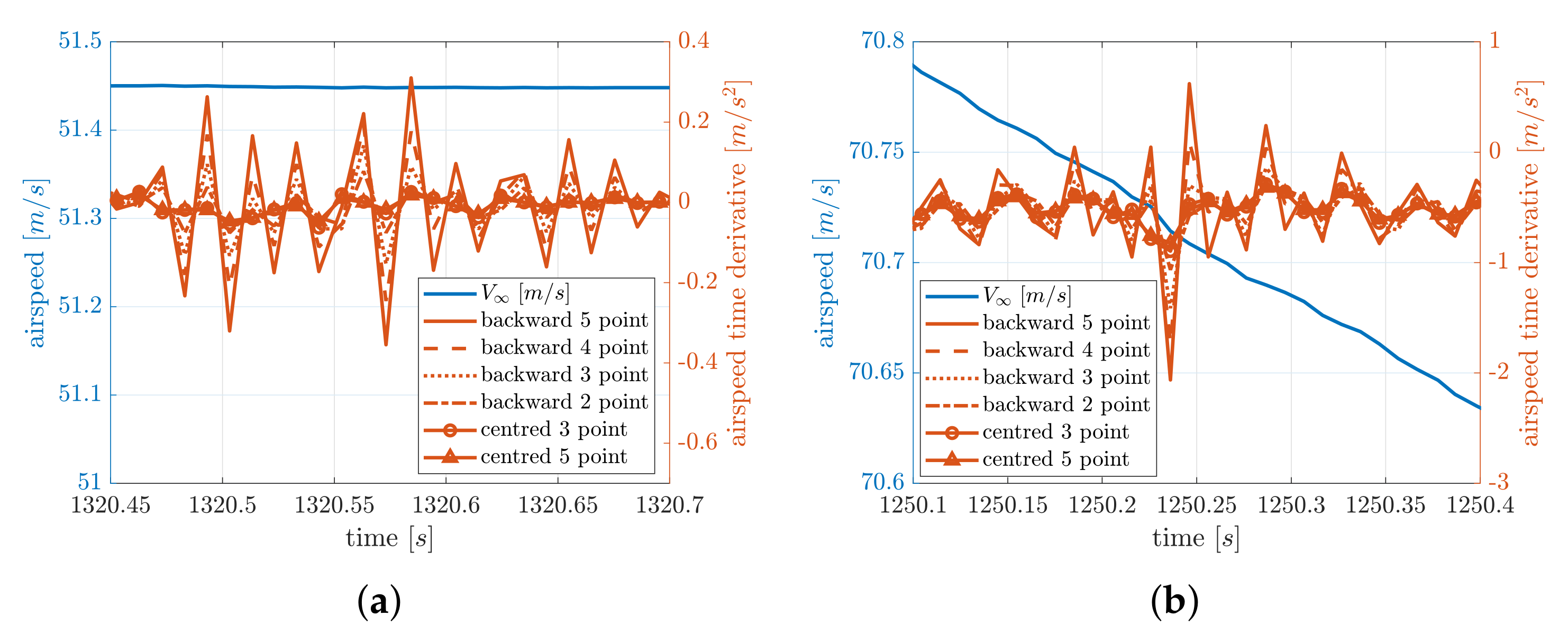
Thirty second time windows with constant airspeed rates are considered in order to evaluate the numerical errors of the airspeed time derivative with respect to the scheme adopted. As can be noted in Figure 10, the more points that are considered in the numerical scheme, the higher the errors. The latter phenomenon is due to the sampling time of the ASSE demonstrator that is not perfectly constant as mentioned before.

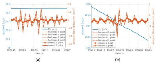
Figure 10. Airspeed time derivative using different numerical schemes. (a) Null TAS rate, ${\dot{V}}_{\infty }=0.01 \mathrm{m} {\mathrm{s}}^{-2}$, (b) Negative TAS rate, ${\dot{V}}_{\infty }=-0.51 \mathrm{m} {\mathrm{s}}^{-2}$.

In Table 1 the error distributions for all the schemes considered in this work are reported.

Table 1. Numerical error analysis using different numerical schemes for airspeed time derivative calculation. With 1σ, 2σ and 3σ is intended the value such that the probability Pr(−σ ≤ X ≤ σ) = 68.3%, Pr(−2σ ≤ X ≤ 2σ) = 95.4% and Pr(−3σ ≤ X ≤ 3σ) = 99.7% also in case the error is not normally distributed.

Mean ${\dot{\mathit{V}}}_{\mathit{\infty }}$	Error $\left({\mathbf{m}\mathbf{s}}^{-2}\right)$	5 Point Backward	4 Point Backward	3 Point Backward	2 Point Backward	5 Point Centred	3 Point Centred
0.01 m s−2	$\sigma$	0.12	0.08	0.06	0.04	0.03	0.03
−0.51 m s−2		0.35	0.28	0.21	0.13	0.11	0.09
−1.00 m s−2		0.69	0.56	0.40	0.25	0.23	0.18
0.01 m s−2	$2\sigma$	0.23	0.17	0.12	0.08	0.07	0.06
−0.51 m s−2		0.67	0.51	0.37	0.23	0.20	0.17
−1.00 m s−2		1.15	0.91	0.72	0.46	0.41	0.35
0.01 m s−2	$3\sigma$	0.35	0.25	0.18	0.12	0.11	0.09
−0.51 m s−2		1.52	1.21	0.95	0.58	0.38	0.31
−1.00 m s−2		3.11	2.55	2.00	1.24	0.76	0.62

Overall, in order to establish the optimal scheme and, hence, the related uncertainty model, a trade-off between static performance (reported in Table 1) and dynamic performance (described in Figure 8) should be carried out. As far as the backward schemes are concerned, the lowest numerical errors are obtained with the 5 point stencil considering the $1\sigma$ error due to the frequency effects of Figure 8b but it shows the largest errors when applied to the ASSE technological demonstrator (Figure 10) for the reasons mentioned before. On the other hand, the 2 point stencil shows the opposite performance: the best performance during steady derivative conditions (Figure 10) and the worst with dynamic derivative conditions (Figure 8). As the present characterisation aims to define an uncertainty budget for the airspeed time derivative, the numerical scheme selection is out of the scope. However, considering the backward schemes, the 3 point backward scheme can be a good compromise between steady state error ($\approx 0.4|{\dot{V}}_{\infty }|$) from Table 1 and the dynamic error ($\approx 0.073 \mathrm{m} {\mathrm{s}}^{-2}$ at 10 $\mathrm{Hz}$) from Figure 8b. Therefore, the total $1\sigma$ uncertainty of the time derivative of the airspeed can be approximated as $1{\sigma }_{{\dot{V}}_{\infty }}=0.073+0.4\left|{\dot{V}}_{\infty }\right|$.

The frequency limit of 10 $\mathrm{Hz}$ is applicable to the majority of modern aircraft, whereas higher frequencies are only limited to very high performance aircraft (e.g., military ones) that should be investigated separately. Moreover, the use of a low-pass filter would also be beneficial to reducing the steady state errors but, at the same time, it would introduce higher delays during dynamic manoeuvres. As said before, the best trade-off should be studied but the latter analysis is out of the present work’s scope.

5. TRL 5 ASSE Verification

As both accelerometers and gyroscope sensors cannot be excited at the same time, the TRL 5 verification of the proposed flow angle synthetic estimator is made up of two complementary activities: (1) integration verification stimulating the accelerometers or the gyroscope along with the air data reproduction, aiming to verify the correct implementation of all necessary algorithms; (2) flight simulations using corrupted data to feed the flow angle synthetic estimator according to noise characterisation introduced in Section 4.

5.1. Integration Verification

The integration verification, or single point verification, aims to verify the correct implementation of all necessary routines and mainly to verify the correct communication interface between the ASSE software module and all other physical sensors. To this purpose, the linearised ASSE scheme of Equation (17) is used because more adequate to the scope. The nonlinear scheme would have required longer time histories of flight manoeuvres that are not feasible in the laboratory environment. In fact, the nonlinear ASSE scheme is tested using flight simulations as reported in Section 5.2.

The test points are designed according to criteria presented in Section 3.2. A first test dataset is conceived, exploiting both the inertial acceleration and the angular rate at the same time as reported in Table 2. The value reported in Table 2 shall be considered as reference values and, therefore, the test results are reported according to the mean values recorded for 1 $\mathrm{s}$ in order to limit the effect of the measurement noise. Moreover, when the flow angle is denoted as N/A it means that the linear scheme of Equation (17) leads to unrealistic values.

Table 2. Numerical ASSE estimation exciting both the accelerometer and the gyroscope with steady state values.

Test #	TAS $\left({\mathbf{m}\mathbf{s}}^{-1}\right)$	${\dot{\mathit{V}}}_{\mathit{\infty }}$ $\left({\mathbf{m}\mathbf{s}}^{-2}\right)$	a ${\left[{\mathit{a}}_{\mathit{X}},{\mathit{a}}_{\mathit{Y}},{\mathit{a}}_{\mathit{Z}}\right]}^{\mathit{T}}$ $\left(\mathit{g}\right)$	$\mathit{\omega }$ ${\left[\mathit{p},\mathit{q},\mathit{r}\right]}^{\mathit{T}}$ $\left(°{\mathbf{s}}^{-1}\right)$	Flow Angle Ref. (AoA, AoS) $\left(°\right)$	Flow Angle Meas. AoA, AoS $\left(°\right)$
1	10	1	${\left[0,1,0\right]}^T$	${\left[0.707,-0.707,0\right]}^T$	N/A, $5.80$	N/A, $5.6$
2	10	2	${\left[0,1,0\right]}^T$	${\left[0.707,-0.707,0\right]}^T$	N/A, $11.6$	N/A, $11.3$
3	10	$2.5$	${\left[0,1,0\right]}^T$	${\left[0.707,-0.707,0\right]}^T$	N/A, $14.6$	N/A, $14.0$
4	10	$1.5$	${\left[0,1,0\right]}^T$	${\left[0.707,-0.707,0\right]}^T$	N/A, $8.8$	N/A, $8.4$
5	10	$-0.5$	${\left[0,0,1\right]}^T$	${\left[-0.707,-0.707,0\right]}^T$	$-2.92$, N/A	$-3.1$, N/A
6	10	$0.25$	${\left[0,0,1\right]}^T$	${\left[-0.707,-0.707,0\right]}^T$	$1.46$, N/A	$1.3$, N/A
7	10	1	${\left[0,0,1\right]}^T$	${\left[-0.707,-0.707,0\right]}^T$	$5.84$, N/A	$5.84$, N/A

Comparing the reference values and the measured values of the flow angles, it is clear that the estimations are implemented correctly even though a residual error can be noted. The latter errors mainly arise because of the deviation from the reference values and those actually realised during the integration tests. For example, considering the test case 1, the value of the reference airspeed time derivative is 1 m s⁻² whereas the mean value obtained during the test with the pressure test set is 0.96 m s⁻² because of the limitation of the experimental setup itself. The deviation of 4% on the ${\dot{V}}_{\infty }$ leads to the 0.2° error on the AoS measurement. On the other hand, the acceleration and the angular rates are affected by very low error as described in Section 4.

A second test dataset is prepared, exploiting both the inertial acceleration and the attitudes at the same time as reported in Table 3. The attitudes are generated using a single axis tilting table. As mentioned before, the main errors arise from the deviation between the air data reference values (TAS and its time derivative) and those actually realised in the laboratory.

Table 3. Numerical ASSE estimation exciting the accelerometer with steady state values.

Test #	TAS $\left({\mathbf{m}\mathbf{s}}^{-1}\right)$	${\dot{\mathit{V}}}_{\mathit{\infty }}$ $\left({\mathbf{m}\mathbf{s}}^{-2}\right)$	Attitudes (Pitch, Roll) $\left(°\right)$	Flow Angle Ref. (AoA, AoS) $\left(°\right)$	Flow Angle Meas. AoA, AoS $\left(°\right)$
8	10	$0.25$	96, 0	N/A, $14.3$	N/A, $13.7$
9	10	$-0.5$	102, 0	N/A, $-14.3$	N/A, $-15.7$
10	10	$0.5$	114, 0	N/A, $7.16$	N/A, $6.9$
11	10	$0.25$	0, 84	$14.4$, N/A	$13.0$, N/A
12	10	$-0.5$	0, 78	$-14.2$, N/A	$-15.1$, N/A
13	10	$0.5$	0, 66	$7.39$, N/A	$7.7$, N/A

Considering the results obtained and reported in Table 2 and Table 3, the communication is correctly implemented between the ASSE software module and all other physical sensors.

5.2. Verification by Simulation

Flight simulated data are obtained using a coupled 6 degree of freedom nonlinear (ultralight) aircraft model equipped with nonlinear aerodynamic and thrust models designed accordingly to flight test results and the engine data sheet. The simulation is run using the explicit Euler scheme with a fixed time step of 10 ms and, therefore, ${\tau }_1=t-10 \mathrm{m}\mathrm{s}$ aiming to simulate the ASSE demonstrator output rate. As the simulator does not implement any sensor noise, all simulated signals are noise-free and synchronised. In order to evaluate preliminarily the ASSE sensitivity to noise, the input signals are corrupted using error models described in Section 4.

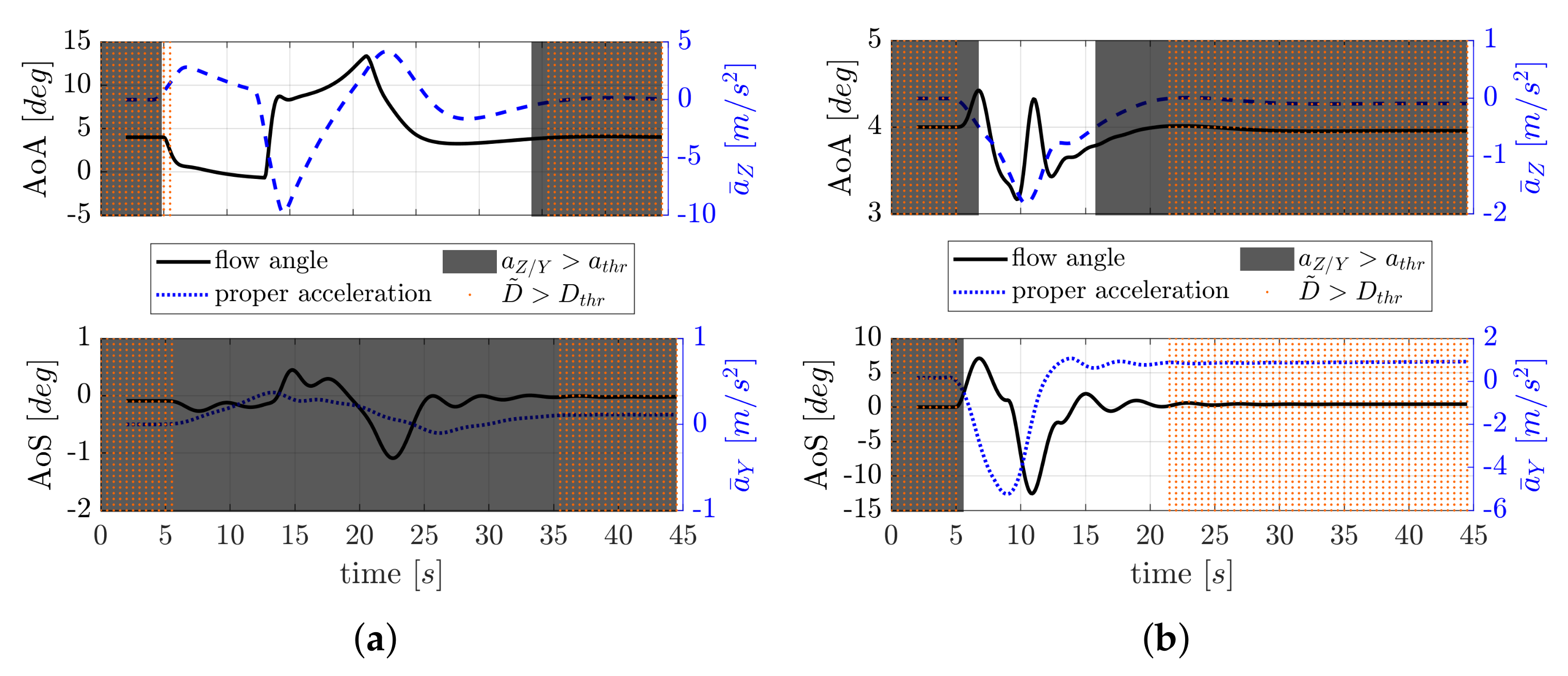
A stall manoeuvre, described in Figure 11a, is performed to excite the AoA up to maximum values. After a short dive, the stall manoeuvre is performed producing initially an increase of airspeed and then a smooth deceleration leading to high angle-of-attack, as can be seen in Figure 11a, with limited changes in angle-of-sideslip and lateral acceleration $a_Y$. The angle-of-sideslip sweep manoeuvre is performed, exciting the angle-of-sideslip in a large range whereas the angle-of-attack is almost constant as can be seen in Figure 11b as well as the vertical acceleration $a_Z$.

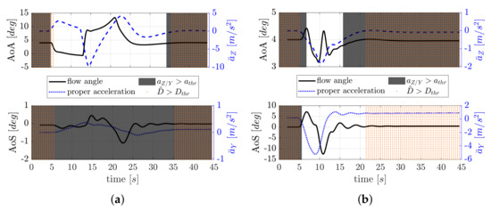
Figure 11. Verification manoeuvres. The shaded areas indicate the regions where the corresponding inertial acceleration modules are below the predefined threshold $a_{thr}$ and dotted areas indicate where the determinant is below a predefined threshold $D_{thr}$. (a) Stall manoeuvre, (b) AoS sweep manoeuvre.

In Figure 11 those flight conditions where the ASSE is not reliable or applicable are indicated. As presented in Section 3.2, some thresholds exist where the analytical ASSE solution cannot be reliable. The criteria of Section 3.2 are sequentially applied. If the absolute value of the inertial acceleration is below the threshold $a_{thr}$, the ASSE scheme leads to unrealistic solutions characterised by very large errors (higher than 5°). The latter condition is represented using dark shaded areas in the Figure 11. Whereas, if $a_Y>a_{thr}$ and/or $a_Z>a_{thr}$, the determinant $\tilde{D}$ is evaluated: if the determinant absolute value is below the threshold $D_{thr}$, the ASSE scheme leads to unreliable solutions where errors up to 5° can be produced. This latter condition is represented using dotted areas in Figure 11. In order to guarantee the flow angle estimation during dynamic manoeuvres, each criteria is considered satisfied only if it is verified for at least 100 consecutive samples, that is, equivalent to 1 $\mathrm{s}$ in this work.

From Figure 11a, it is clear that the AoS cannot be estimated during the stall manoeuvre using the ASSE scheme because the lateral acceleration is below the defined threshold $a_{thr}$ and the AoS is around the null value. Whereas, the AoA can be estimated using the ASSE scheme in the time window [5 s, 34 s]. As far as the AoS sweep manoeuvre is concerned, the AoA can be estimated in the time window [6 s, 17 s]. On the other hand the AoS could be estimated in the time window [5 s, 45 s] but accepting less reliability from 21 s onwards.

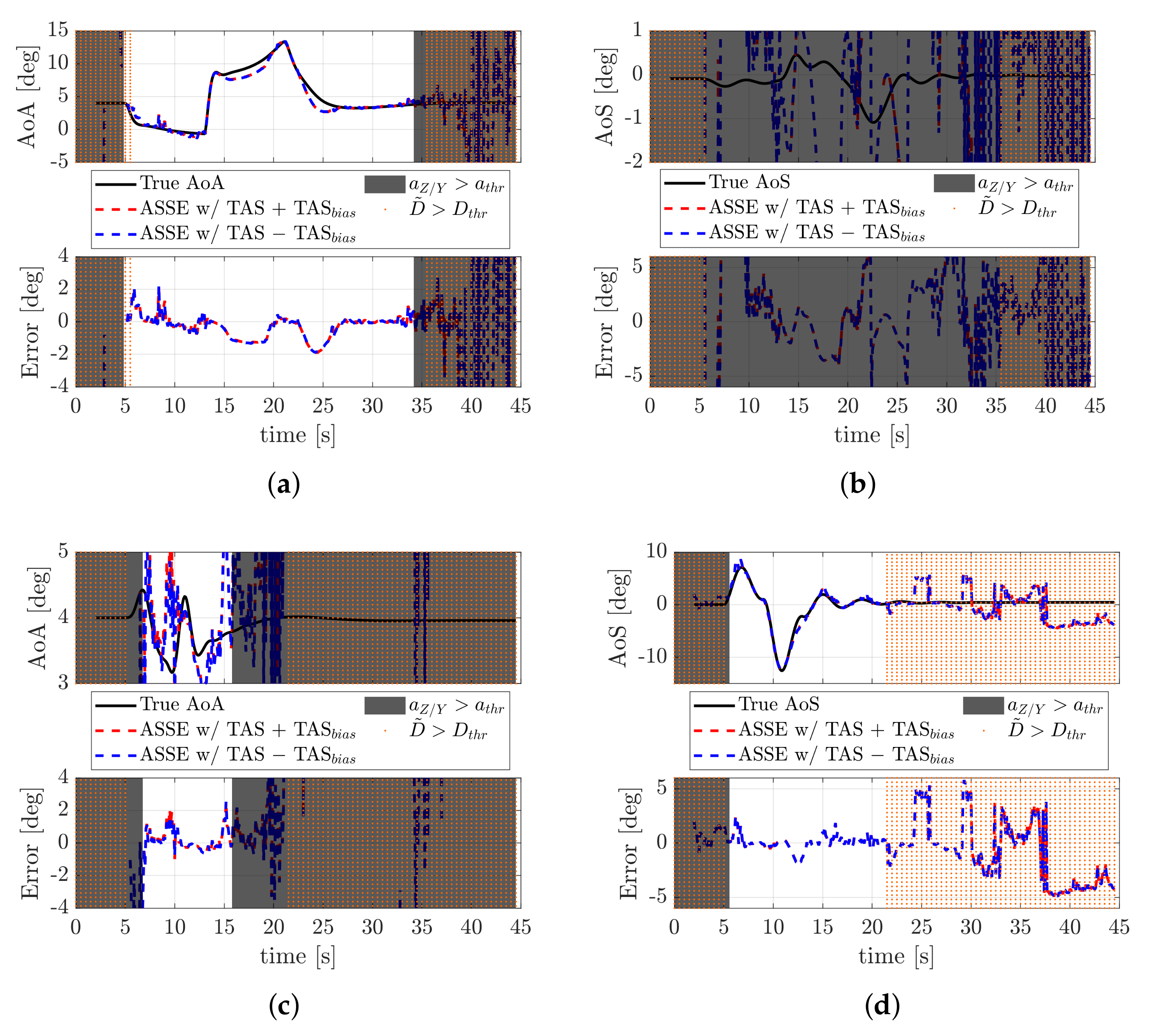
Results of the AoA and AoS estimations using the nonlinear ASSE scheme are presented in Figure 12. First of all, it can be noted that the sign of the CAS bias does not play a significant role as both the dashed red (TAS_bias = 0.47 m s⁻¹) and blue (TAS_bias = −0.47 m s⁻¹) lines are not distinguishable.

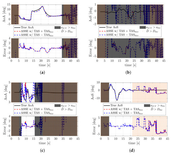
Figure 12. AoA and AoS estimation using the nonlinear ASSE scheme during the verification manoeuvres. The shaded areas indicate the regions where the corresponding inertial acceleration modules are below the predefined threshold $a_{thr}$ and the dotted areas indicate where the determinant is below a predefined threshold $D_{thr}$. (a) AoA estimation during the stall manoeuvre, (b) AoS estimation during the stall manoeuvre, (c) AoA estimation during the sweep manoeuvre, (d) AoS estimation during the sweep manoeuvre.

As said before, during the stall simulation, the AoS cannot be estimated using the nonlinear ASSE scheme as can be observed in Figure 12b. In fact, except for a very limited time range between 12 s and 20 s where the error estimation is below ±5°, the error is not acceptable. On the other hand, the AoA is estimated with adequate accuracy in the time window [5 s, 34 s] as the error is always below ±2.5°. However, the AoA estimation is less accurate at the beginning of the manoeuvre (time ≈ 5 s) where the determinant criteria are not satisfied even if the acceleration criteria are satisfied. These latter considerations, as also observed in [27], limit the application of the ASSE scheme at the beginning of the manoeuvre because the scheme relies on previous time steps (related to steady-state conditions) and, hence, not significant equations are considered in the scheme to be solved. Therefore, a preliminary conclusion leads to consider the determinant condition crucial, that is, as important as the acceleration criteria, when the manoeuvre begins.

As far as the AoS sweep manoeuvre is concerned, the vertical acceleration $a_Z$ is small, even though it is beyond the threshold in the time window [6 s, 17 s] where the ASSE scheme is used to estimate the AoA as in Figure 12c. Even though the estimation is not very accurate, the error is bounded in ±2.5°, which is acceptable for the scope of the present work. On the other hand, the AoS estimation can be performed with the nonlinear ASSE scheme for the entire manoeuvre except for the initial steady state conditions where the acceleration criteria are not met. However, from ≈22 s the determinant criteria are not met and, in fact, large errors (up to ±5°) can be noted. It is worth noting that, when the $\tilde{D}>D_{thr}$ the AoS estimation is biased with respect to the true value.

The error analysis proposed in Table 4 does not have a general validity on the performance of the ASSE scheme for AoA and AoS estimation because it would require the simulation of a whole flight envelope that is practically impossible. Moreover, a better strategy should be defined to take into account the conclusions of the present work. In fact, the proposed error analysis is intended to provide an overview of the ASSE possible performance in a realistic simulated environment (as required for TRL 5 validation) along with the integration verification tests.

Table 4. ASSE estimation error analysis of the mean, absolute maximum, $1\sigma$ and $2\sigma$ errors. With $1\sigma$ and $2\sigma$ the value is intended such that the probability $Pr\left(-\sigma \le X\le \sigma \right)=68.3\%$ and $Pr\left(-2\sigma \le X\le 2\sigma \right)=95.4\%$ also in case the error is not normally distributed.

Flow Angle	ASSE Exclusion Criteria	Mean Error $\left(°\right)$	Max Abs. Error $\left(°\right)$	$1\mathit{\sigma }$ Error $\left(°\right)$	$2\mathit{\sigma }$ Error $\left(°\right)$
AoA	$\tilde{D}<D_{thr}$ OR $a_{Y,Z}<a_{thr}$	−0.19	3.02	0.60	1.66
	$a_{Y,Z}<a_{thr}$	0.18	3.02	0.61	1.67
AoS	$\tilde{D}>D_{thr}$ OR $a_{Y,Z}>a_{thr}$	0.04	2.52	0.41	1.74
	$a_{Y,Z}>a_{thr}$	−0.52	5.80	2.11	4.73

At first sight, the OR condition between the determinant and the acceleration criteria would lead to more accurate results only because the ASSE scheme is applied to less flight data where the conditions are more suitable. However, it should be noted that the very large AoA maximum error is mainly due to the transition at the beginning of the stall manoeuvre (Figure 12a). On the other hand, the large AoS maximum error is experienced when the AoS values are quite constant and null as can be noted in Figure 12d, leading to a large $2\sigma$ as well.

Therefore, from the proposed results and error analysis, the OR condition should be preferred to achieve very low errors ($2\sigma < 2°$). Moreover, more stringent performance requirements on the flow estimation would require other solvers as mentioned before, rather than an iterative approach to solve the nonlinear ASSE scheme.

6. Conclusions

Within the scenario of flow angle synthetic estimators, the project SAIFE’s scope is to design and manufacture a suitable technological demonstrator in order to verify at TRL 5 a model-free approach for flow angle estimation. The proposed approach is based on the rearrangement of classical flight mechanic equations in order to obtain a set of nonlinear equations, or the ASSE scheme. As the proposed scheme is only applicable when the aircraft is manoeuvring, practical thresholds are used to identify the flight conditions where the flow angle estimation is more reliable. The technological demonstrator is able to provide all necessary inputs to the ASSE scheme: true airspeed, angular rates, inertial accelerations and aircraft attitudes. In the present work, the inputs provided by physical sensors are characterised in order to evaluate the uncertainty budget on the performed measurements. This latter aspect is crucial for testing the nonlinear ASSE scheme in a realistic scenario for the TRL 5 verification. Firstly, the technological demonstrator is tested in the laboratory both to evaluate the uncertainty budget of the physical sensors and to verify the correct implementation of the required algorithms. Secondly, the ASSE scheme is tested using flight simulations data that are corrupted with realistic uncertainties. In order to tolerate the uncertainties of the input signals, 200 nonlinear equations are used to define the ASSE scheme, that is, data collected for 2 $\mathrm{s}$. The latter choice highly depends on the physical sensors used and, therefore, on the particular aircraft application. The numerical results show low errors with $2\sigma < 2°$ both for AoA and AoS that are within the initial objectives. It is worth noting that results of the present work can be applied to any flying body to estimate the flow angles as the proposed ASSE scheme is model-free. On the other hand, the proposed setup relies on iterative methods to solve a scheme of 200 nonlinear equations and is unlikely to fit with a practical implementation. Further investigations are required to solve the ASSE scheme using alternative solvers that, for example, may contribute to reducing the number of nonlinear equations.

References

- Norris, G. Enhanced angle-of-attack system set for 737-10 flight test. Aviat. Week Space Technol. 2021. Available online: https://aviationweek.com/shownews/dubai-airshow/enhanced-angle-attack-system-set-737-10-flight-tests (accessed on 30 November 2021).
- SAE International. Minimum Performance Standards, for Angle of Attack (aoa) and Angle of Sideslip (AOS); SAE International: Warrendale, PA, USA, 2019. [Google Scholar]
- Vitale, A.; Corraro, F.; Genito, N.; Garbarino, L.; Verde, L. An Innovative Angle of Attack Virtual Sensor for Physical-Analytical Redundant Measurement System Applicable to Commercial Aircraft. Adv. Sci. Technol. Eng. Syst. J. 2021, 6, 698–709. [Google Scholar] [CrossRef]
- Ariante, G.; Ponte, S.; Papa, U.; Del Core, G. Estimation of Airspeed, Angle of Attack, and Sideslip for Small Unmanned Aerial Vehicles (UAVs) Using a Micro-Pitot Tube. Electronics 2021, 10, 2325. [Google Scholar] [CrossRef]
- Prem, S.; Sankaralingam, L.; Ramprasadh, C. Pseudomeasurement-aided estimation of angle of attack in mini unmanned aerial vehicle. J. Aerosp. Inf. Syst. 2020, 17, 603–614. [Google Scholar] [CrossRef]
- Valasek, J.; Harris, J.; Pruchnicki, S.; McCrink, M.; Gregory, J.; Sizoo, D.G. Derived angle of attack and sideslip angle characterization for general aviation. J. Guid. Control. Dyn. 2020, 43, 1039–1055. [Google Scholar] [CrossRef]
- Lerro, A.; Battipede, M.; Gili, P.; Ferlauto, M.; Brandl, A.; Merlone, A.; Musacchio, C.; Sangaletti, G.; Russo, G. The clean sky 2 MIDAS project—An innovative modular, digital and integrated air data system for fly-by-wire applications. In Proceedings of the 2019 IEEE 6th International Workshop on Metrology for AeroSpace (MetroAeroSpace), Turin, Italy, 19–21 June 2019; Volume 1, pp. 714–719. [Google Scholar] [CrossRef]
- Gertler, J. Analytical redundancy methods in fault detection and isolation - survey and synthesis. IFAC Proc. Vol. 1991, 24, 9–21. [Google Scholar] [CrossRef]
- Perhinschi, M.; Campa, G.; Napolitano, M.; Lando, M.; Massotti, L.; Fravolini, M. Modelling and simulation of a fault-tolerant flight control system. Int. J. Model. Simul. 2006, 26, 1–10. [Google Scholar] [CrossRef]
- Pouliezos, A.D.; Stavrakakis, G.S. Analytical Redundancy Methods; Springer: Amsterdam, The Netherlands, 1994; Volume 12, pp. 93–178. [Google Scholar] [CrossRef]
- Rhudy, M.B.; Fravolini, M.L.; Porcacchia, M.; Napolitano, M.R. Comparison of wind speed models within a Pitot-free airspeed estimation algorithm using light aviation data. Aerosp. Sci. Technol. 2019, 86, 21–29. [Google Scholar] [CrossRef]
- Eubank, R.; Atkins, E.; Ogura, S. Fault detection and fail-safe operation with a multiple-redundancy air-data system. In AIAA Guidance, Navigation, and Control Conference; American Institute of Aeronautics and Astronautics: Reston, VA, USA, 2010; pp. 1–14. [Google Scholar] [CrossRef] [Green Version]
- Lu, P.; Van Eykeren, L.; Van Kampen, E.J.; Chu, Q. Air data sensor fault detection and diagnosis with application to real flight data. In AIAA Guidance, Navigation, and Control Conference; AIAA SciTech Forum: Reston, VA, USA, 2015; pp. 1–18. [Google Scholar] [CrossRef]
- Komite Nasional Keselamatan Transportasi Republic of Indonesia. Aircraft Accident Investigation Report - PT. Lion Mentari Airlines Boeing 737-8 (MAX). KNKT.18.10.35.04. 2018. Available online: http://knkt.dephub.go.id/knkt/ntsc_aviation/baru/2018-035-PK-LQPFinalReport.pdf (accessed on 30 November 2021).
- European Aviation Safety Agency. Easy Access Rules for Unmanned Aircraft Systems; EASA: Cologne, Germany, 2015. [Google Scholar]
- European Aviation Safety Agency. Proposed Means of Compliance with the Special Condition VTOL; MOC SC-VTOL; Issue 1; EASA: Cologne, Germany, 2020. [Google Scholar]
- Estrada, M.A.R.; Ndoma, A. The uses of unmanned aerial vehicles—UAV’s- (or drones) in social logistic: Natural disasters response and humanitarian relief aid. Procedia Comput. Sci. 2019, 149, 375–383. [Google Scholar] [CrossRef]
- Radoglou-Grammatikis, P.; Sarigiannidis, P.; Lagkas, T.; Moscholios, I. A compilation of UAV applications for precision agriculture. Comput. Networks 2020, 172, 107148. [Google Scholar] [CrossRef]
- Baniasadi, P.; Foumani, M.; Smith-Miles, K.; Ejov, V. A transformation technique for the clustered generalized traveling salesman problem with applications to logistics. Eur. J. Oper. Res. 2020, 285, 444–457. [Google Scholar] [CrossRef]
- Dendy, J.; Transier, K. Angle-of-Attack Computation Study; Technical Report AFFDL-TR-69-93; Air Force Flight Dynamics Laboratory: Wright-Patterson AFB, OH, USA, 1969. [Google Scholar]
- Freeman, D.B. Angle of Attack Computation System; Technical Report AFFDL-TR-73-89; Air Force Flight Dynamics Laboratory: Wright-Patterson AFB, OH, USA, 1973. [Google Scholar]
- Rohloff, T.J.; Whitmore, S.A.; Catton, I. Air data sensing from surface pressure measurements using a neural network method. AIAA J. 1998, 36, 2094–2101. [Google Scholar] [CrossRef]
- Samara, P.A.; Fouskitakis, G.N.; Sakellariou, J.S.; Fassois, S.D. Aircraft angle-of-attack virtual sensor design via a functional pooling narx methodology. IEEE Eur. Control. Conf. 2003, 1, 1816–1821. [Google Scholar] [CrossRef]
- Wise, K.A. Computational Air Data System for Angle-of-Attack and Angle-of-Sideslip. U.S. Patent 6,928,341 B2, 2005. [Google Scholar]
- Langelaan, J.W.; Alley, N.; Neidhoefer, J. Wind field estimation for small unmanned aerial vehicles. J. Guid. Control. Dyn. 2011, 34, 1016–1030. [Google Scholar] [CrossRef]
- Lu, P.; Van Eykeren, L.; van Kampen, E.; de Visser, C.C.; Chu, Q.P. Adaptive three-step kalman filter for air data sensor fault detection and diagnosis. J. Guid. Control. Dyn. 2016, 39, 590–604. [Google Scholar] [CrossRef] [Green Version]
- Lerro, A.; Brandl, A.; Gili, P. Model-free scheme for angle-of-attack and angle-of-sideslip estimation. J. Guid. Control. Dyn. 2021, 44, 595–600. [Google Scholar] [CrossRef]
- Lerro, A.; Brandl, A.; Gili, P.; Pisani, M. The SAIFE Project: Demonstration of a Model-Free Synthetic Sensor for Flow Angle Estimation. In Proceedings of the 2021 IEEE 8th International Workshop on Metrology for AeroSpace (MetroAeroSpace), Naples, Italy, 23–25 June 2021; pp. 98–103. [Google Scholar] [CrossRef]
- Lacondemine, X.; Barbier, D. In-Flight Demonstration of a LiDAR Based Air Data System DANIELA Project. In Proceedings of the Sixth European Aeronautics Days (Aerodays), Madrid, Spain, 30 March–1 April 2011. [Google Scholar]
- Lerro, A. Survey of certifiable air data systems for urban air mobility. In Proceedings of the 2020 AIAA/IEEE 39th Digital Avionics Systems Conference (DASC), San Antonio, TX, USA, 11–15 October 2020; pp. 1–10. [Google Scholar] [CrossRef]
- Schmidt, D. Modern Flight Dynamics; McGraw-Hill: New York, NY, USA, 2011. [Google Scholar]
- Etkin, B.; Reid, L. Dynamics of Flight: Stability and Control, 3rd ed.; Wiley: Hoboken, NJ, USA, 1995. [Google Scholar]
- Lerro, A.; Brandl, A.; Gili, P. Neural network techniques to solve a model-free scheme for flow angle estimation. In Proceedings of the 2021 International Conference on Unmanned Aircraft Systems (ICUAS), Athens, Greece, 15–18 June 2021; pp. 1187–1193. [Google Scholar] [CrossRef]
- Lerro, A. Physics-based modelling for a closed form solution for flow angle Estimation. Adv. Aircr. Spacecr. Sci. 2021, 8, 273–287. [Google Scholar] [CrossRef]
- Marquardt, D.W. An algorithm for least-squares estimation of nonlinear parameters. J. Soc. Ind. Appl. Math. 1963, 11, 431–441. [Google Scholar] [CrossRef]
- Lerro, A.; Musacchio, C. Preliminary definition of metrological guidelines for synthetic sensor verification. In Proceedings of the 2020 IEEE 7th International Workshop on Metrology for AeroSpace (MetroAeroSpace), Pisa, Italy, 22–24 June 2020; pp. 187–192. [Google Scholar] [CrossRef]
- Pisani, M.; Astrua, M. The new INRIM rotating encoder angle comparator (REAC). Meas. Sci. Technol. 2017, 28, 045008. [Google Scholar] [CrossRef]
- Pisani, M.; Astrua, M.; Iafolla, V.; Santoli, F.; Lucchesi, D.; Lefevre, C.; Lucente, M. On-ground actuator calibration for ISA—BepiColombo. In Proceedings of the 2015 IEEE Metrology for Aerospace (MetroAeroSpace), Benevento, Italy, 4–5 June 2015; pp. 312–317. [Google Scholar] [CrossRef]
- Chung, T.J. Solution methods of finite difference equations. In Computational Fluid Dynamics; Cambridge University Press: Cambridge, UK, 2002; pp. 63–105. [Google Scholar] [CrossRef]
Publisher’s Note: MDPI stays neutral with regard to jurisdictional claims in published maps and institutional affiliations. |
© 2022 by the authors. Licensee MDPI, Basel, Switzerland. This article is an open access article distributed under the terms and conditions of the Creative Commons Attribution (CC BY) license (https://creativecommons.org/licenses/by/4.0/).