Abstract
A substantial amount of money and time is required to optimize resources in a massive Wi-Fi network in a real-world environment. Therefore, to reduce cost, proposed algorithms are first verified through simulations before implementing them in a real-world environment. A traffic model is essential to describe user traffic for simulations. Existing traffic models are statistical models based on a discrete-time random process and combine a spatiotemporal characteristic model with the varying parameters, such as average and variance, of a statistical model. The spatiotemporal characteristic model has a mathematically strict assumption that the access points (APs) have approximately similar traffic patterns that increase during day times and decrease at night. The mathematical assumption ensures a homogeneous representation of the network traffic. It does not include heterogeneous characteristics, such as the fact that lecture buildings on campus have a high traffic during lectures, while restaurants have a high traffic only during mealtimes. Therefore, it is difficult to represent heterogeneous traffic using this mathematical model. Deep learning can be used to represent heterogeneous patterns. This study proposes a generative model for Wi-Fi traffic that considers spatiotemporal characteristics using deep learning. The proposed model learns the heterogeneous traffic patterns from the AP-level measurement data without any assumptions and generates similar traffic patterns based on the data. The result shows that the difference between the sample generated by the proposed model and the collected data is up to 72.1% less than that reported in previous studies.
1. Introduction
A substantial amount of money and time is required to design a new network and to optimize resources of an already established network in a real-world environment. Therefore, for cost reduction, proposed algorithms are first verified through simulations before being implemented in a real-world environment. Modeling and simulation techniques are among the most prevalent methods used during this verification process [1].
For articulating real traffic, traffic models have been widely employed. Traffic modeling is a widely researched topic in studies on networks. A traffic model considers the randomness of the user and the spatiotemporal-varying traffic load. Traffic is modeled as a statistical model based on a discrete-time random process and combines a spatiotemporal characteristic model with the varying parameters (e.g., average and variance) of the statistical model [2,3,4]. For example, in modeling session arrivals, the session arrival is a discrete-time random process, where the arrival time of the session and the identity of the AP are unknown. Furthermore, the session arrival rate increases during the daytime and decreases at night. Many researchers usually adopt a Poisson process to model the session arrival. Difference researchers employ different methods to model the spatiotemporal characteristics of the session arrival. Hernández-Campos et al. [3] modeled the time-varying rate function for the Poisson parameter. This model assumed a slowly varying arrival rate that increased during daytime and decreased at night. Ghosh et al. [4] modeled the rate function , where J denoted the time slots dividing 24 h and I denoted the tag of the cluster grouped by the average number of arrivals. This model assumed that was a linear function. Therefore, previous studies have modeled the spatiotemporal characteristics with a strict assumption that ensures the homogenization of network traffic.
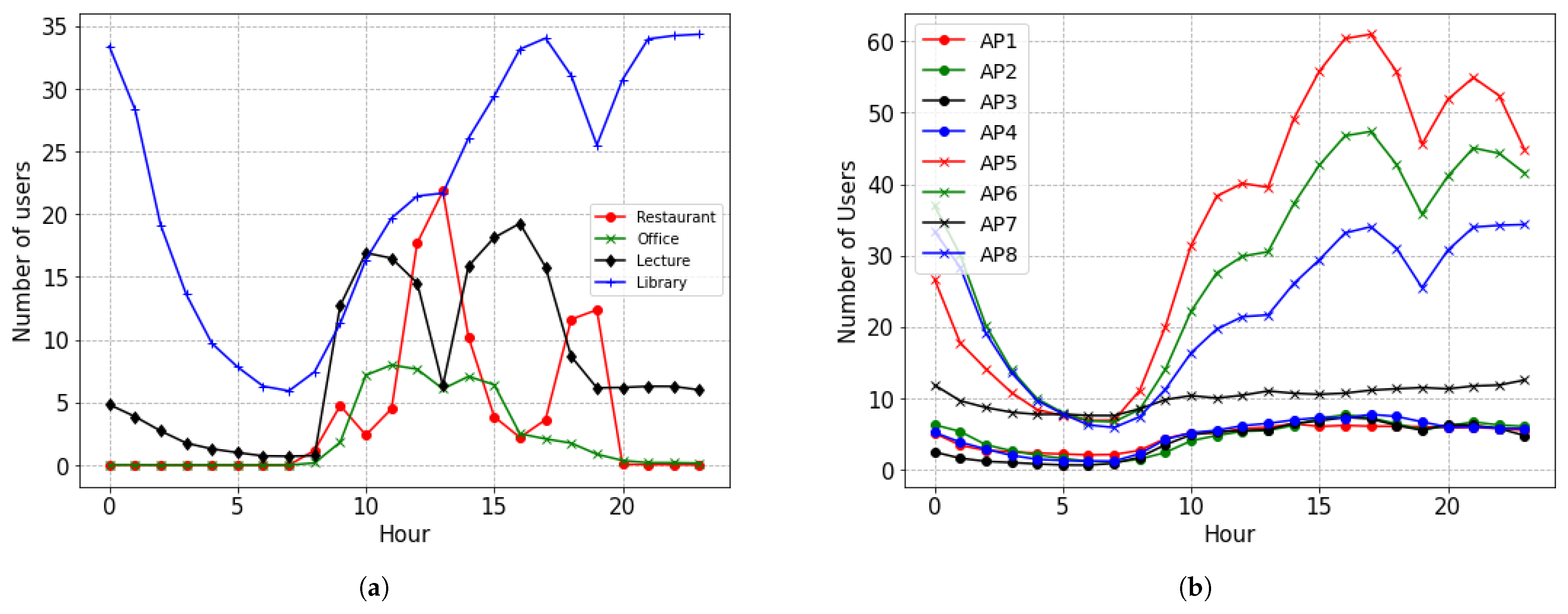
The spatiotemporal characteristics of the traffic are heterogeneous in terms of the AP-level. Figure 1 shows the changing number of users collected from the APs installed on the campus of Pusan National University (PNU) located in Pusan, South Korea. Figure 1a shows the changing number of sessions over time upon selecting an AP from different buildings. Each AP has a different pattern for the number of users. In the restaurant, the number of users increases at mealtime. In the office, users associate the Wi-Fi system during daytime except for lunchtime. In the lecture building, the pattern of the number of users is similar to that of the office, but the volume of the pattern is large. The library has more users at night than during the daytime. Figure 1b shows the changing number of users over time for all APs placed on a floor in the library. All APs have similar patterns, but the volume difference between the APs is significant. APs 5, 6, and 8 have a pattern in which the number of users changes considerably and the number of users falls at mealtime. The remaining APs have less variations in their number of users. Upon examining the Wi-Fi system at the AP level, the heterogeneity of the spatiotemporal characteristics can be observed.

Figure 1.
Heterogeneity of the number of sessions. (a) Changing number of sessions over time by selecting an AP from different buildings that display different patterns. This is because the time of concentration of users varies depending on the use of the building. (b) Changing number of users for all APs on a floor in the library. The APs have a similar pattern, but the volume difference is significant.
Previous studies are limited in regard to representing heterogeneous traffic patterns owing to the strict assumptions. In other words, mathematical assumptions make traffic patterns homogeneous. The model for a time-varying session arrival is a typical example of such patterns. In addition, some studies classify the use of buildings to complement the homogeneity of traffic patterns. However, it takes a considerable time and effort to select a suitable mathematical model for the use of the building and all the APs in the building.
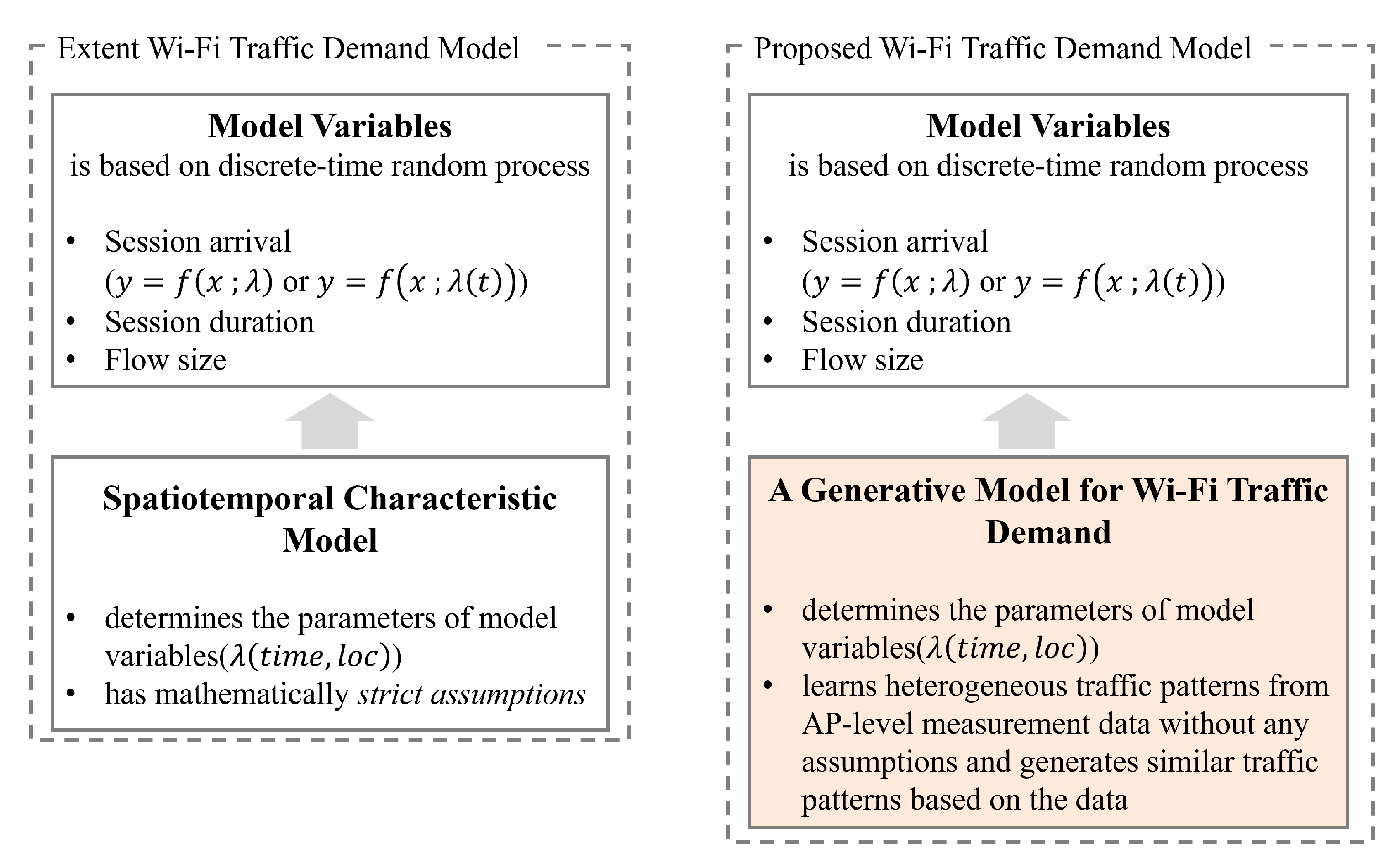
Deep learning can be used to represent heterogeneous patterns. In particular, the generative model learns the patterns of the input and produces samples similar to the input [5,6,7]. Therefore, this study proposes a generative model for Wi-Fi traffic demand by employing machine learning. This model possesses spatiotemporal characteristics. Wi-Fi traffic pattern changes over time and varies from site to site. Each site has a different traffic volume depending on the purpose of site. A difference in the traffic volume between the APs was observed even on the same site depending on the location of the AP within one site and the usage of the installed site. Figure 2 shows the distinction between our proposal and extent studies. Existing traffic demand models are divided into determining model variables based on a discrete-time random process and the spatiotemporal characteristic model. This study replaces the spatiotemporal characteristic model with the spatiotemporal characteristic generative model.
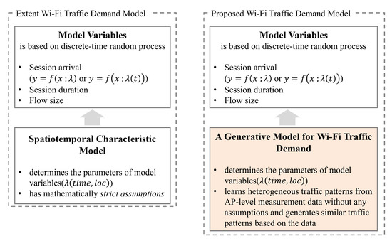
Figure 2.
The distinction between existing studies and the Wi-Fi traffic generative model. Existing traffic demand models are divided into determining model variables based on a discrete-time random process and the spatiotemporal characteristic model. This study replaces the spatiotemporal characteristic model with the spatiotemporal characteristic generative model.
This study proposes a new unit of Wi-Fi usage, which is a measurement vector of the AP level. Each metric can be used for the simulation or as a constant average rate for existing traffic models. The traffic pattern is represented as a three-dimensional tensor using the Wi-Fi usage with the shape of time, AP, and usage.
The contributions are as follows:
- First, this study proposes a new Wi-Fi usage measure to represent the traffic pattern. Each attribute of the Wi-Fi usage can be used either for the simulation or as a constant average rate for existing traffic models.
- Second, this study proposes a generative model for Wi-Fi traffic demand. This model trains the spatiotemporal characteristics of the Wi-Fi usage and generates the patterns of Wi-Fi traffic on site.
- Finally, this study evaluates the performance of the generative model for Wi-Fi traffic demand. The evaluation compares the distributions of samples that are produced by the model and the data collected from the site.
The remainder of this article is structured as follows. Section 2 reviews existing studies on mathematical traffic and traffic prediction models based on deep learning. Section 3 introduces the generative model for Wi-Fi traffic demand based on deep learning. This study proposes three models: spatial, temporal, and spatiotemporal. Section 4 evaluates the proposed models. The performance evaluation compares the distribution of samples produced by the model and data obtained from the site. Section 5 discusses the interpretation of the performance of the proposed model. Section 6 summarize the paper and presents further challenges.
2. Related Work
2.1. Modeling Spatiotemporal Characteristics in Network Traffic
Several existing spatiotemporal models include mathematically strict assumptions [3,4,8,9,10,11,12]. Hernández-Campos et al. [3] modeled traffic data collected from a campus-wide Wi-Fi system. Session and flow data were collected for eight days at 5 min intervals from approximately 500 APs. The model variables were session arrival, AP of the first association per session, flow interarrival per session, flow number per session, and flow size. In particular, the rate of the session arrival varied over time. Therefore, the session arrival modeled the rate over time. The rate was high during working hours and low at night when there were fewer people. This study assumed that the arrival rate changed slowly over time. This assumption made it difficult to model sudden changes in session arrival, such as lunchtime in restaurants. Additionally, it homogenized the changes in session arrival over time, such as increasing in the morning and decreasing in the afternoon.
Ghosh et al. [4] modeled traffic data collected in different places: coffee shops, fast-food restaurants chains, bookstores, hotels, and enterprises. The study modeled traffic through approximately 1.3 million sessions collected over four weeks; the model variables were session arrival, connection time, and simultaneous users. Unlike the study conducted by Hernández-Campos et al. [3], this study analyzed the spatial characteristics for the model variables. The arrival distribution in coffee shops had three peaks, which were around 9 a.m., 1 p.m., and 7 p.m. Although the traffic size varied depending on the size of the site, the traffic featured three peaks, and the arrival distribution on weekdays and weekends depicted different patterns. The connection time varied according to the type of the sites. Coffee shops or fast-food restaurant chains recorded the lowest average connection time, while the average connection time for bookstores and hotels was the longest. Despite considering spatial factors, the study was limited owing to the design of model variables with strict assumptions.
Some studies have tackled homogeneous traffic patterns. In order to consider more aspects of spatial characteristics, these studies have set more complex mathematical assumptions. Ding et al. [9] modeled the connection density and traffic distribution for mobile networks in large cities. The spatial distribution of the model was modeled as log-normal, and the spatial distribution was classified according to the purpose of the site through clustering. However, the spatial characteristics of this model did not reach the level of grasping the relationship between base stations (BS). Marvi et al. [10] modeled traffic demand assuming a heterogeneous traffic scenario wherein a user could generate multiple flows for different services. In the real world, for privacy reasons, it is difficult for network managers to know what applications users are using in the network. Wang et al. [11] models temporally and spatially fluctuated traffic. This study also considered this application. Zhang et al. [12] modeled mobile traffic patterns using a generative advertising network (GAN). However, GAN is difficult to sample because it is modeled on implicit latent variables among generative models.
2.2. Network Traffic Model Based on Deep Learning
Recently, several studies have approached the traffic prediction problem by considering the spatiotemporal characteristics based on deep learning [13,14,15,16,17,18,19,20,21]. The traffic prediction problem deals with the estimation of traffic at time through past traffic of duration L. This problem is represented as . Wang et al. [13] targeted a cellular network covering an area of 6500 km. They predicted the traffic load over a cycle of one hour by dividing the space into a grid of size 500 × 500 m. This model included a neighbor grid to predict the traffic load of the target grid. Moreover, the temporal characteristics were modeled using a long short-term memory (LSTM) network. He et al. [14] predicted the traffic load in Milan, Italy. They collected traffic data that were sampled at intervals of 10 min in 100 × 100 grids of size 235 m × 235 m. They observed that the grid-based model was appropriate for expressing relationships with neighboring grids, but there was a limit to expressing two similar traffic patterns separated by some distance. To solve this problem, they adopted a graph-based model for the spatial characteristics. Furthermore, they used a recurrent neural network (RNN), a time-series prediction model that focused on the temporal factors [22]. Fang et al. [15] predicted traffic demand from more than 6000 cells with an average of 3 million subscribers per day. It was performed based on individual cells, from data collection to modeling. Graph convolution (GC) was used for modeling the spatial characteristics. GC is a type of neural network that aggregates the node information of neighbors using a graph structure [23]. Since graphs are useful for expressing the topology of a network, there have been many deep learning studies that reflect spatial characteristics using GC [24,25]. The LSTM and GRU have been used to model the temporal characteristics [13,14,16,26].
Previous studies confirm that deep learning is an excellent technology that can be used for modeling spatiotemporal traffic patterns. This study attempts to apply deep learning for traffic modeling. However, prediction models are difficult to use. Network traffic modeling, which generates traffic for specific conditions, differs from prediction modeling in that it requires the information of the past n steps. A traffic prediction model is a many-to-one mapping. The generative model, which is an one-to-many mapping, is suitable for traffic modeling. However, it is rare for generative models to be applied to traffic modeling. There are only a few intrusion detection studies [27,28,29] that have used the generative model. From a system management perspective, some studies, such as the one conducted Xiao et al. [30], infer a QoS or synthesize a traffic matrix for network management, such as the one by Kakkavas et al. [31]. The major contribution of this study is the application of generative models to traffic modeling.
Recently, the generative model [32,33] has been used for modeling traffic models. A variational autoencoder (VAE) is an explicit probabilistic model to generate structured outputs in generative models. Figure 3 shows the structure of a VAE that consists of an encoder network that encodes interpretable features of input X into a latent variable z and a decoder network that generates the sample , which possesses more similarities with X than with z. It is assumed that z usually follows a normal distribution. An encoder network models the approximate posterior distribution . The goal of this network is to obtain which approximates .
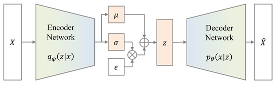
Figure 3.
Variational autoencoder. an encoder network that encodes the interpretable features of an input X into a latent variable z and a decoder network that generates a sample that has more similarities with X than with z.
3. Modeling of Traffic Demand
This study proposes a traffic demand modeling method that divides the modeling into three parts: session arrival, session throughput, and user localization. The session arrival models when the station (STA) arrives at the AP. The session throughput models the amount of traffic used by the session. The user location models the distance and angle between the AP and STA. This study performs the three proposed modeling at the AP level. Moreover, the three proposed modeling parts require parameters for each AP. Therefore, a generative model for Wi-Fi traffic demand is proposed to provide the appropriate parameters for each AP and time.
3.1. Wi-Fi Usage
Traffic can be expressed with various metrics, including its throughput. Throughput is a general metric representing the traffic volume of the Wi-Fi users. However, there is a lack of representation of the Wi-Fi user demand using only amount of traffic. User demand combines the spatial characteristics of the placement of the users. It can be used to consider the placement of additional APs when establishing future Wi-Fi management strategies. Therefore, Wi-Fi user demand must be expressed in the form of a vector that combines multiple metrics. This study defines the Wi-Fi usage in terms of the throughput, number of users, and average received signal strength indicator (RSSI)
Equation (1) defines the Wi-Fi usage vector of an AP. The vector values consist of the metrics that are used for the simulation. The number of users is set in the simulation itself or used as a constant average rate of the session arrival model. The average RSSI is a value obtained by averaging the RSSI measured at the AP for all users. This value is used to determine the position of users using the path loss model [34]. The throughput is the average throughput of all sessions. This value is used to determine the volume of traffic.
3.2. Model Variables
Session arrival has a periodic pattern based on the day, as shown in the graph in Figure 1. The arrival of the session is modeled as an AP-level, nonstationary, time-dependent Poisson process. APs have different patterns depending on the use of the building and different scales. Thus, the Poisson distribution requires rate parameters, which are modeled as time-varying: . provides the value of the number of users in the Wi-Fi usage vector corresponding to the rate of session arrival on an AP i at time t.
Throughput is modeled as a log-normal distribution. Figure 4b shows the distribution of throughput with time for an AP in the library. The time was selected as 07:00, which has the lowest throughput, along with the three peak times of 01:00, 16:00, and 22:00. The majority of the throughput at 07:00 is close to 0, forming a heavy-tail distribution. The high throughput rates at 01:00 or 16:00 are also skewed on average.
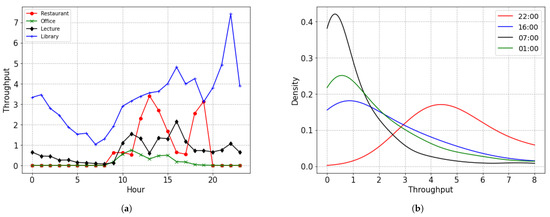
Figure 4.
Heterogeneity of throughput. (a) Change in the throughput with time upon selecting APs from different buildings. Different buildings have different patterns. This is because the time of concentration for the user varies depending on the use of the building. (b) Densities for an AP in a library at different times.
The throughput at 22:00 is close to a normal distribution with a high average. Figure 4a shows the change in the throughput over time for different buildings. The throughput pattern is similar to the pattern of the number of users, as shown in Figure 1a. Accordingly, the throughput is modeled to change the rate over time, such as the number of connected people.
User localization models the distance and angle between the STA and AP. The user location is an attribute required for AP relocation. When a user is concentrated on a specific site, it is necessary to determine whether an AP must be at the site. The distance is obtained using a path-loss model with the average RSSI modeled as a normal distribution. The distribution of the collected data has a similar distribution at the same time.
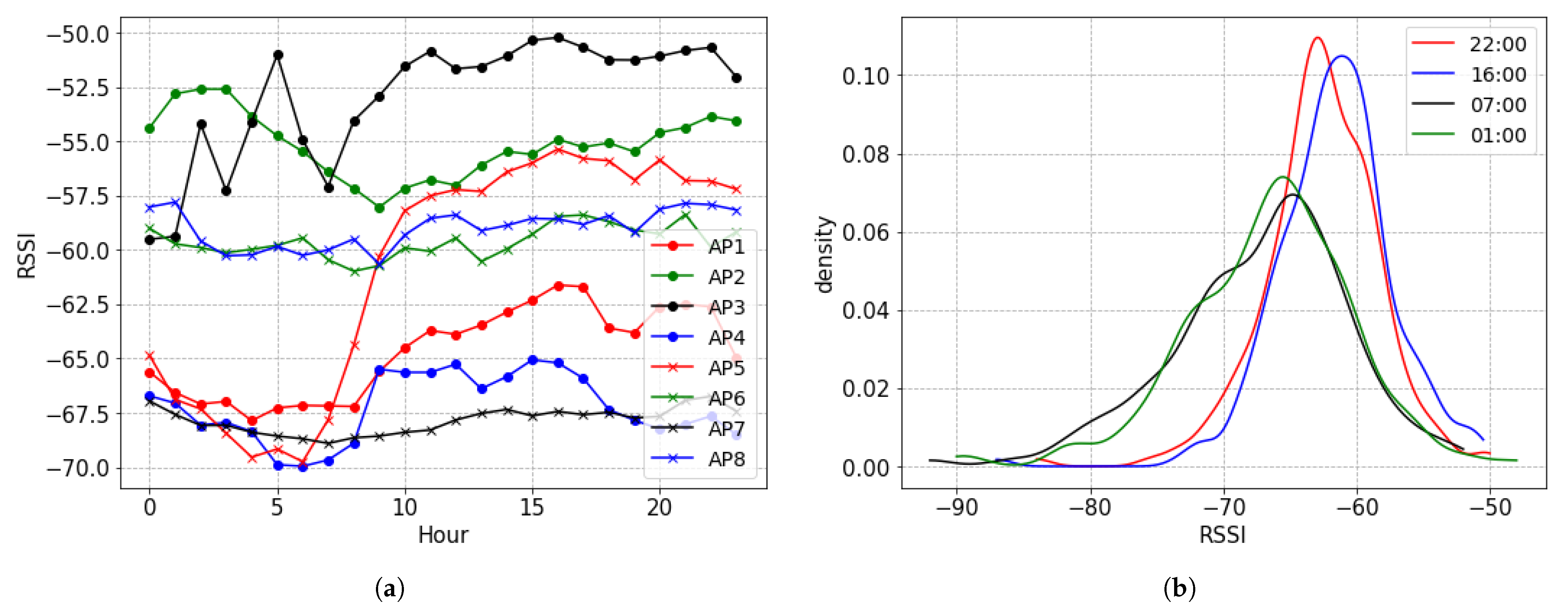
Figure 5 shows the distribution of the RSSI and change in the RSSI with time. Figure 5b shows the densities for an AP in a library at different times. It follows a normal distribution. Figure 5a shows the changing average RSSI over time for AP selection from different buildings. The average RSSI does not have the same periodicity of the day as the throughput. Rather, the RSSI values are similar at all times. This implies that it has a more significant influence on the position of the STA than user concentration. In such a case, it is more challenging to model the temporal characteristics.

Figure 5.
Heterogeneity of the RSSI. (a) Change in the RSSI with time for AP selections from different buildings. The RSSI does not have the same periodicity over the day as the throughput. Rather, the RSSI values are similar at all times. This implies that it has a more significant influence on the position of the STA than user concentration. (b) Densities for an AP in a library at different times. It follows a normal distribution.
3.3. Problem Formulation for Wi-Fi Traffic Demand Generation
Using the definition of the Wi-Fi usage pattern, the demand generation of Wi-Fi traffic configures the usage per AP at a site based on its history. The demand generation for Wi-Fi traffic is represented in Equation (2). The model generates Wi-Fi usage patterns when the latent variable z is the input. This study intends for z to approximate the distribution in the relationship between the APs over time. An interference matrix I represents the interference of the AP with other APs. The Wi-Fi usage pattern is generated considering an interference relationship between the APs at a site.
3.4. Interference Matrix
The relationship of the interference between APs at a site can be represented as a graph where a node refers to an AP and an edge indicates the interference. If two APs do not interfere with each other, the Wi-Fi usage of the two APs is not affected by each other. The interference matrix I is represented in Equation (3).
The path-loss model is used to calculate the communication range of the AP. The received signal strength is represented by , where is the transmission power of the node j and and are the antenna’s gain of transmission and reception, respectively. The loss of signal strength over distance is represented by [34], where is the distance of the APs i and j, is the frequency in use, is the number of walls, and is the number of floors. In this study, the generative model for the Wi-Fi traffic demand creates patterns for a floor, hence, . Equation (4) is derived by combining the above equations. is the communication range of the node j. When a received signal strength is , the distance is given by
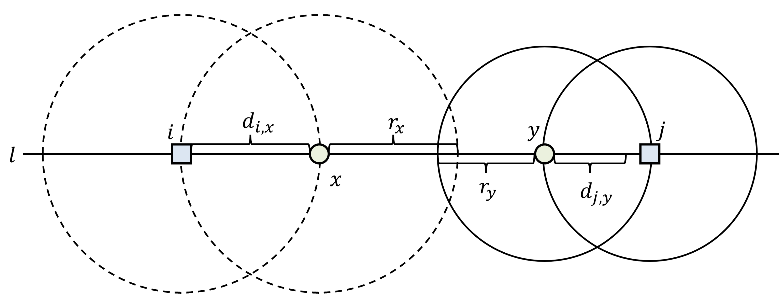
To determine whether APs i and j interfere each other, STAs x and y associated with APs i and j, respectively, are virtually created, as shown in Figure 6. Let the straight line connecting the APs i and j be L. The virtual STAs are placed at the point where the communication range of the two APs meets the straight line L. If is larger than , the two links and interfere with each other. Therefore, this model determines that AP i and j interfere with each other.
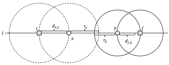
Figure 6.
Interference range between AP i and j [35]. Two virtual STAs x and y from AP i and j, respectively, are placed the closest. If the two links and do not interfere, a link interference between APs i and j does not occur.
3.5. Wi-Fi Traffic Demand Generative Model
3.5.1. Spatial Modeling—Variational Graph Autoencoder (VGAE)
GC is an operation that converts nodes included in a graph or a graph itself into a vector [36]. The graph is represented by , where is an adjacency matrix indicating the connection to each node, is the node feature matrix, N is the number of nodes in the graph, and d is the dimension of the node feature vector. GC creates a new feature matrix receiving A and X, where m is the dimension of the latent feature vector. The GC operation is represented by Equation (5), where is a trainable weight matrix. Training the GC is equivalent to adjusting the weight matrix. The activation function is used to generate a nonlinear output, such as a sigmoid or rectified linear unit (ReLU).
There are two limitations to using the adjacency matrix A. First, A indicates only the connections with neighboring nodes; the information about the node itself is not considered when creating a latent feature vector. Second, because A is not regularized, the size of the feature vector may become unstable when multiplied by the adjacency matrix A. To solve the two problems, a self-loop is added to the adjacency matrix A, and A is regularized to where D is the degree matrix of A. Equation (6) represents the adjacency matrix which adds the self-loop S.
Furthermore, the regularized GC is represented as Equation (7), where is the degree matrix of
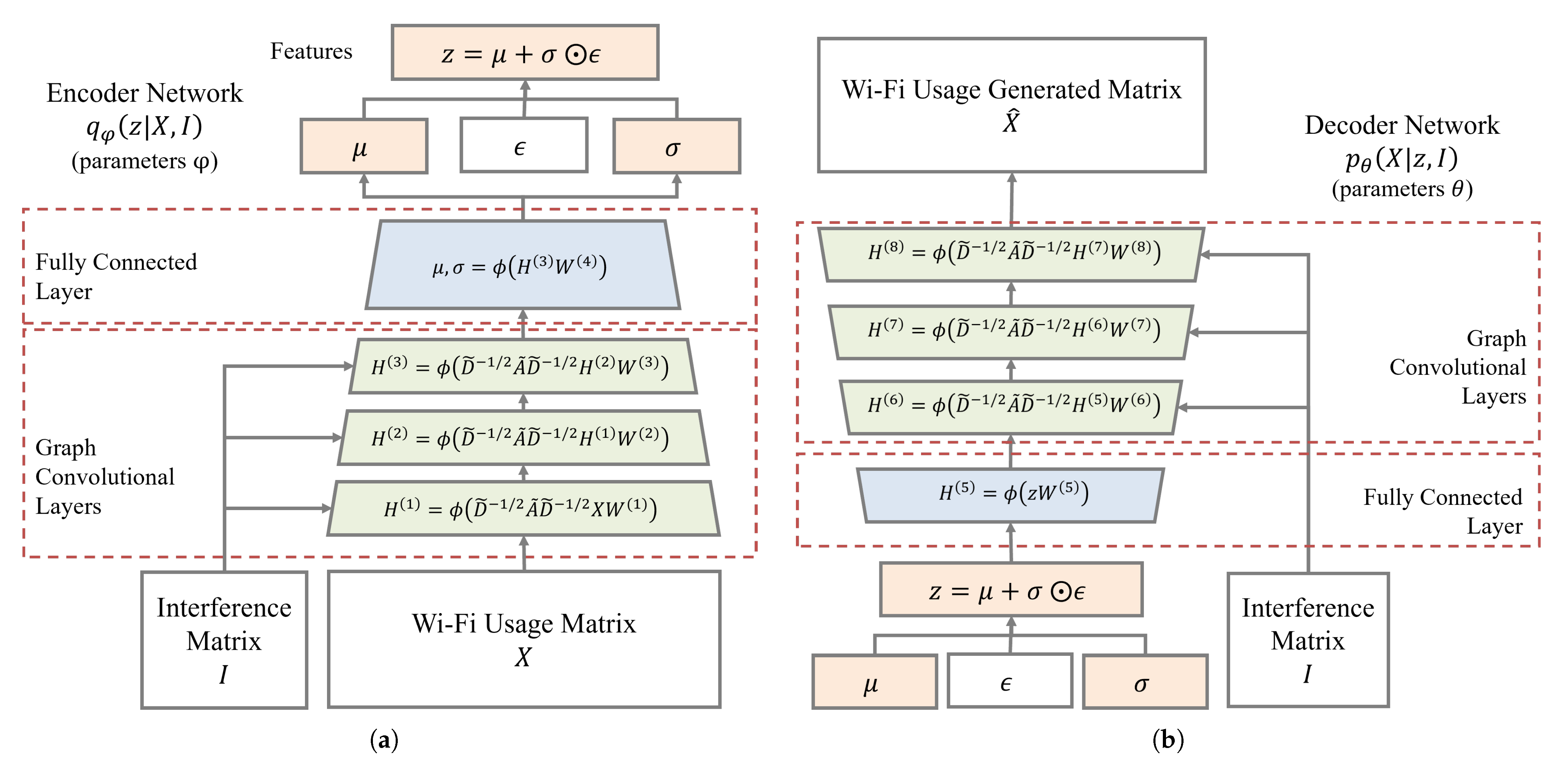
This study first proposes a variational graph autoencoder (VGAE), which uses GC to model spatial characteristics. This model consists of encoder and decoder networks. Figure 7a illustrates an encoder network. This model trains the probability that approximates the distribution in the relationship between APs over time, where X represents Wi-Fi usage patterns, I is the interference matrix, and z represents latent variables. This model consists of 3 GC layers and a fully connected (FC) layer. The GC layer encodes the spatial features of a site and is represented in Equation (8). The FC layer encodes the spatial features into latent variables z.
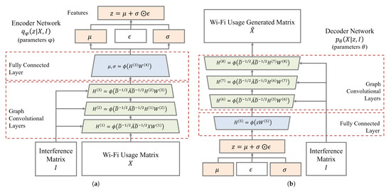
Figure 7.
Variational graph autoencoder: (a) encoder, (b) decoder. The encoder network encodes the spatial features of Wi-Fi usage patterns into latent variables z. The decoder network generates Wi-Fi usage patterns from the latent variables z.
Figure 7b illustrates a decoder network. This model trains the probability , which is a probability of generating a sample from latent variables z where I is the adjacency matrix. This model consists of an FC layer and three GC layers. The FC layer decodes the latent variables into spatial features. Three GC layers decode the spatial features into sample .
3.5.2. Temporal Model—Variational Recurrent Autoencoder (VRAE)
RNNs are used to train on the relationship of time series data [37]. The RNN is designed to capture sequential information in data, such as audio and natural language. In particular, the RNN adds a feedback path to the feedforward neural network. Thus, the current output is related to the present and past inputs. However, the problem with widely known standard RNNs is the limitation in modeling long-term dependencies [38]. LSTM is a unit operation that solves the long-term dependency limitations of existing RNNs [39]. Additionally, a gated recurrent unit (GRU) is also a recurrent unit operation that is more straightforward than the LSTM operation [40]. In this study, the GRU was used to learn the pattern of time-series data. There is no significant difference in structure and performance between the LSTM and GRU [41]. It does not imply that there is no significant difference in the performance but that either the LSTM or GRU is better depending on the subject. However, it is a definite advantage that a GRU has a small trainable weight.
Unlike a RNN, the GRU has gates that determine how much the previous and current information has been updated. A GRU has a reset gate and an update gate . The reset gate uses a sigmoid function as an output to multiply the value by the previously hidden layer to reset the previous information. The reset gate is calculated, as shown in Equation (9). is obtained by multiplying the previous hidden layer feature with the weights and the current input with the weights .
The update gate determines the update ratio of the previous and current features. The update gate is calculated as shown in Equation (10). is obtained by multiplying the previous hidden layer feature with the weights and the current input with the weights . and are used to determine the amount of and to be updated, respectively.
The candidate gate for the current information is represented in Equation (11). is used by multiplying with . ⊙ denotes the element-wise multiplication.
Finally, is calculated, as shown in Equation (12). It is obtained by multiplying the candidate by the update gate and the previous hidden features by .
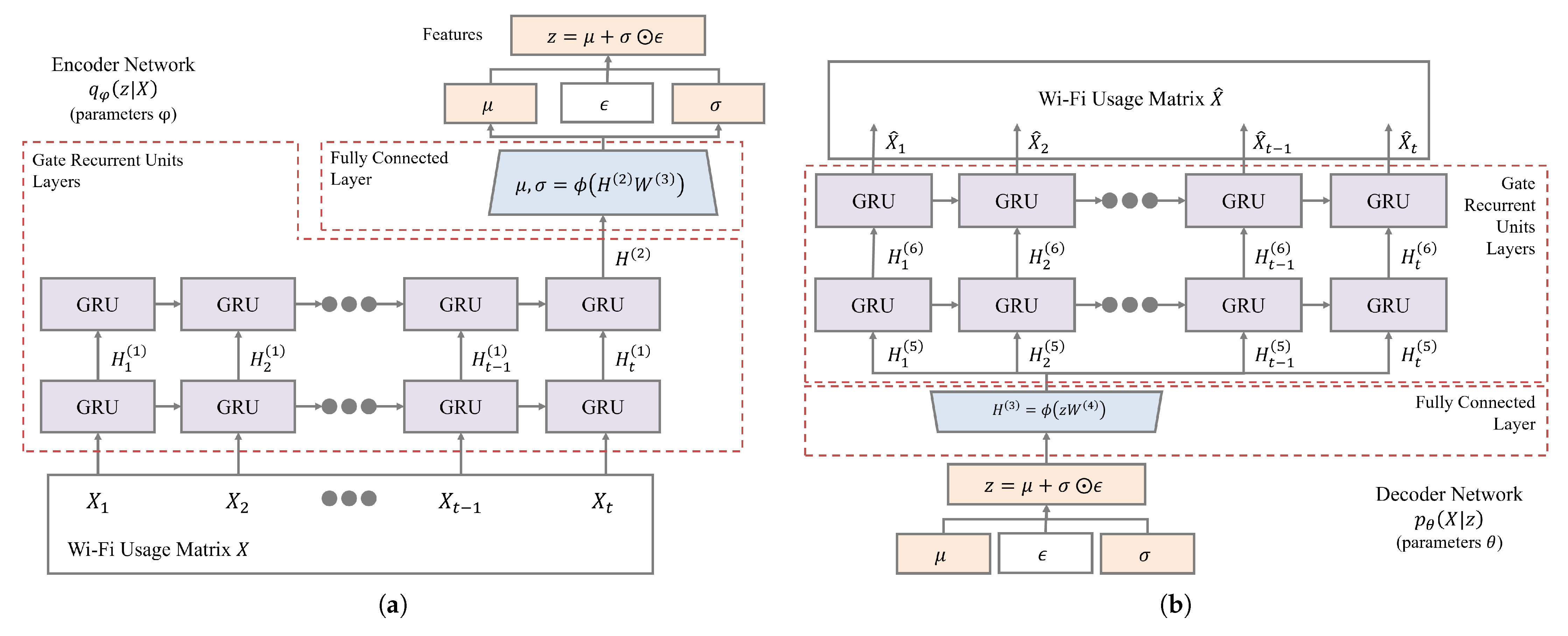
This study proposes a variational recurrent autoencoder (VRAE), which uses the GRU to model the temporal characteristics. Figure 8a illustrates an encoder network. The VRAE does not use the adjacency matrix I because this model is intended to train only temporal characteristics. This model consists of two GRU layers and an FC layer. The GRU layer encodes the temporal features of the Wi-Fi usage, as expressed in Equation (13). The decoder network is illustrated in Figure 8b; it reverses the order of the encoder network and consists of two GRU layers and one FC layer.
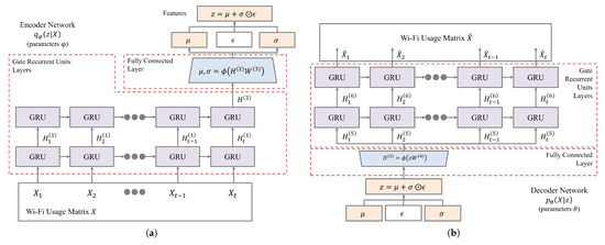
Figure 8.
Variational recurrent autoencoder: (a) encoder, (b) decoder. The encoder network encodes the temporal features of Wi-Fi usage patterns into latent variables z. The decoder network generates Wi-Fi usage patterns from the latent variables z.
3.5.3. Spatiotemporal Model—Variational Recurrent Graph Autoencoder (VRGAE)
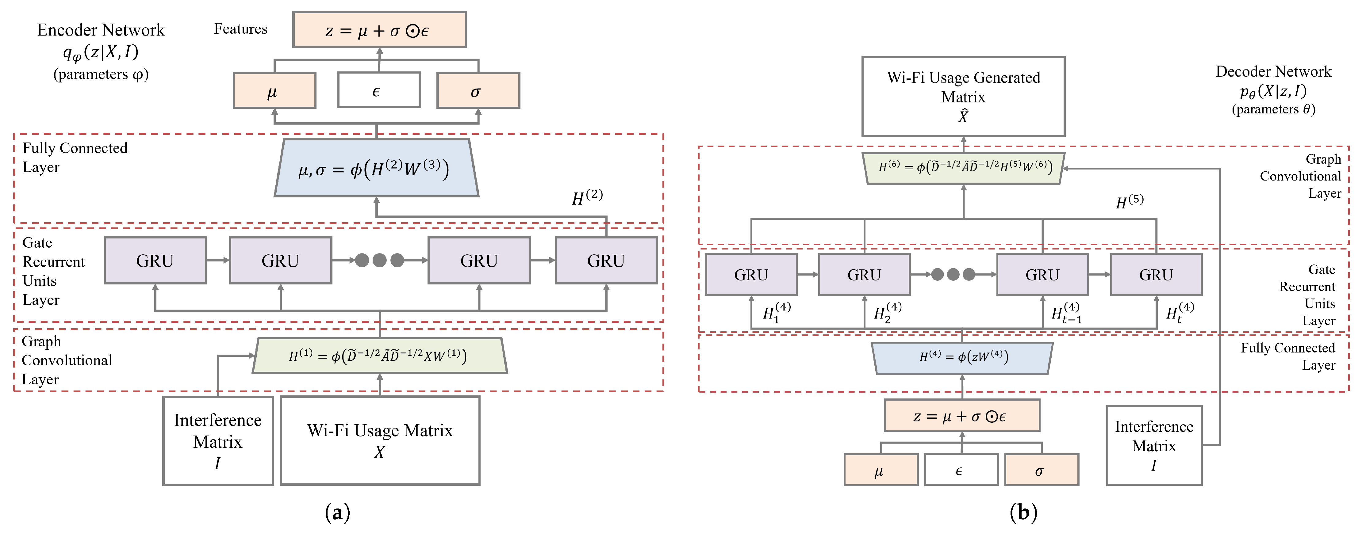
This study proposes a variational recurrent graph autoencoder (VRGAE), which models the spatial characteristics using the GC and temporal characteristics using the GRU. This model consists of a GC, a GRU, and an FC layer. Reducing the number of GC and GRU layers compared with the previous two proposed models ensures the number of trainable variables are similar. In addition, it is intended to improve the performance with the structure of the model while maintaining the number of weights.
The VRGAE is illustrated in Figure 9 and operates in the following manner.
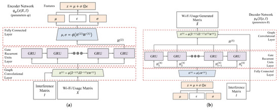
Figure 9.
Variational recurrent graph autoencoder: (a) encoder, (b) decoder. The encoder network encodes the spatiotemporal features of Wi-Fi usage patterns into latent variables z. The decoder network generates Wi-Fi usage patterns from the latent variables z.
- Encoder
- Layer 1:
- Layer 2:
- Layer 3:
- Decoder
- Layer 4:
- Layer 5:
- Layer 6:
Layer 1 performs the GC to encode the spatial characteristics of Wi-Fi usage patterns. An input of this layer is Wi-Fi usage pattern and an interference matrix I, where T is the number of time slot, N is the number of AP, F is the length of Wi-Fi usage, and is an activation function. The number of trainable weight is , which is the same as the shape of . Layer 2 performs the GRU to encode the temporal characteristics. An input of this layer is the output of the previous layer . The number of trainable weights is . Layer 3 performs an FC to encode the spatiotemporal features into latent variables. An input of this layer is the output of the previous layer , where is an activation function. The number of trainable weights is .
Layer 4 performs the FC to decode the latent variables into spatiotemporal features. The inputs of this layer are the latent variables , where and are the average and standard deviation of a normal distribution, respectively, and , sampled from a normal distribution, adds random noise used to maintain a degree of disorder in z. Layer 5 performs the GRU to decode the temporal characteristics. An input of this layer is the output of the previous layer . The number of trainable weights is . Layer 6 performs the GC to decode the Wi-Fi usage patterns from temporal features. An input of this layer is and I.
4. Performance Evaluation
4.1. Data Collection and Scale
The data collection consisted of measurements obtained from the APs operated by PNU. It has a total of 92 buildings on campus. The total area is 1.4 km and there are approximately 30,000 people including students and faculty members. The network equipment on campus is manufactured by Cisco corporation. The campus has 1622 APs, both indoors and outdoors [42]. The status of the APs was measured from 00:00 on 1 June 2019, to 23:00 on 31 December 2020, in consultation with the IT center of PNU. The total number of records was 8,330,592. This study collected AP measurements hourly along with spatial information. The spatial information coordinates the wall and position of the APs based on the floor plan of the building.
Table 1 provides an example of an hourly AP measurement. The AP measurement integrates samples measured in units of 5 min. The information category in the table includes information on the AP, namely its name, internet protocol (IP) address, medium access control (MAC) address, location, and measurement time of the AP. The measurement category includes many metrics. The number of users was an average value for all samples. The RSSI and signal-to-noise ratio (SNR) were average values for all users. The throughput was obtained by determining the total bytes transmitted and received in one hour.

Table 1.
Attributes for AP Measurement.
This section evaluates how similar samples generated from the models are to those from the dataset. There were three performance evaluations. The first evaluation compared the distribution between the previous and proposed models. The second evaluation compared the distributions between the proposed models themselves. The third evaluation compared the distributions of each site between the sample data and the dataset. This classified sites according to the performance of the generative models and analyzed traffic patterns at each site.
4.2. Comparison between Existing Studies
The first evaluation compared the performance of the proposed model and existing models. The evaluation compared the difference between the distribution of the sample data and the distribution of the collected data—the smaller difference between the two distributions, the better the model’s performance. The maximum mean discrepancy (MMD) is a metric representing the difference between two distributions.
The MMD was used as an indicator for evaluating the two distributions. The MMD is a metric that compares two distributions defined in the same domain [43]. If the distributions for a domain X are defined as p and q, the MMD can be defined according to Equation (14). x and are independently distributed according to the data distribution p. y and are distributed according to the data distribution q. is a kernel function, and this paper used Gaussian kernels. x and are sampled from the dataset distribution p, and y and are sampled from the sample data distribution q of the generative model.
As shown in Figure 1, the traffic demand had different patterns depending on the site, and there was a difference in volume between the APs at the same site with the same pattern. Therefore, the performance of the model characterized firstly the MMD between APs installed at different sites and secondly the MMD between multiple APs at the same site. Figure 10 represents the MMD measured from the two perspectives.
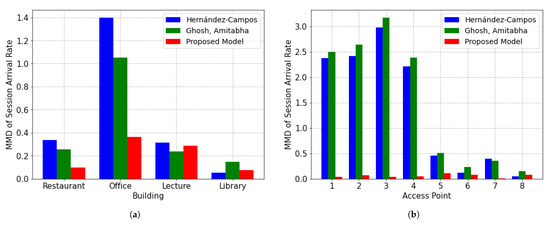
Figure 10.
Comparison between collected data and samples generated by the model. (a) MMD of one AP located in a different building. (b) MMD of all APs located in a floor of the library.
As shown in Figure 10a, the models compare the MMDs with APs installed in different buildings. The proposed model records a low MMD in restaurants and offices. Restaurants have increased traffic characteristics at mealtimes. Previous studies had a hard time representing the characteristics of the restaurant’s traffic due to a strict assumption that it increases at work time and decreases at night. The office has a higher MMD than that of other sites. The reason is that there is a significant difference in traffic volume between weekends and weekdays. For example, at 15:00, the difference between weekends and weekdays is significant. However, the models cannot consider weekends and weekdays, so they cannot distinguish between weekends and weekdays. The lecture hall and library have similar performances to the previous models.
Figure 10b represents the MMD for all APs on a floor of the library. The proposed model indicates that the sample data of each AP are similar to a dataset. In previous models, APs 5 to 8 generate samples similar to the datasets, but APs 1 to 4 do not. As shown in Figure 10a, APs 1 to 4 have low traffic volumes, and APs 5 to 8 have high traffic volumes. It shows that aggregating the traffic of all APs, which is the limitation of the statistical model, makes it hard to represent the traffic pattern of each AP.
4.3. Comparison between Proposed Models
The second evaluation compared the distributions between the sample data generated from the proposed models and the dataset. Models to be evaluated were VAE, VGAE, VRAE, and VRGAE. For the evaluation, in addition to the proposed models, a VAE was added. VAE does not include the spatiotemporal characteristics. This model consists of FC layers. VGAE, VRAE, and VRGAE consider the spatial characteristics, temporal characteristics, and all characteristics, respectively. By comparing the performance of these models, the similarity of the dataset with respect to the structure of the model can be observed.
When defining part of the entire service area of the Wi-Fi system in the campus scale as a site, the unit of site was defined as a floor, and thus, the Wi-Fi system was divided into 260 sites. This study compared the dataset and sample data for each site using the average MMD (AMMD), which was calculated in Equation (15). This equation averages the MMD for the site index .
The AMMD of the proposed models is shown in Figure 11. The more spatiotemporal characteristics considered in the models, the smaller the difference from the dataset. Spatial characteristics have more influence on the AMMD reduction than temporal characteristics. The AMMD of VGAE is 0.843, which is a reduction of approximately 45% from that of the VAE, but the AMMD of VRAE is 0.909, which is a reduction of approximately 41% from that of VAE. This evaluation suggested that the generative model could generate Wi-Fi traffic patterns well. The VAE demonstrated excellent performance for a one-to-many mapping that generates Wi-Fi usage patterns. In addition, it was confirmed that more similar samples could be generated when considering the spatiotemporal characteristics in generating Wi-Fi usage patterns.
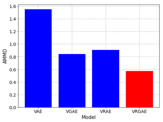
Figure 11.
Comparison of the AMMD between the proposed models. The more generative models consider the characteristics of a site, the more similar the samples generated are. Spatial characteristics have a more significant influence on the distribution of samples than temporal characteristics. Considering both characteristics, the VRGAE produces samples most similar to the datasets.
4.4. Comparison of the Distribution of Each Site
The third evaluation compared the distributions of each site between the sample data and the dataset. The VRGAE, which exhibits the best performance among the proposed models, was used for the evaluation. The number of sites was 260 floors on the campus of PNU. Figure 12 shows the MMD for each site. It ranges from the lowest MMD site at 0.02 to the highest at 4.69. By observing the MMD values of the sites, some similar MMD sites can be clustered into similar characteristics. The low MMD value of some sites can not only be attributed to the similarity in the distributions of the sample data generated by the model and the dataset, but also to the low Wi-Fi usage. A site with a low Wi-Fi usage means that most values converge to 0, and there is no change in the usage over time or any difference in the usage between APs.
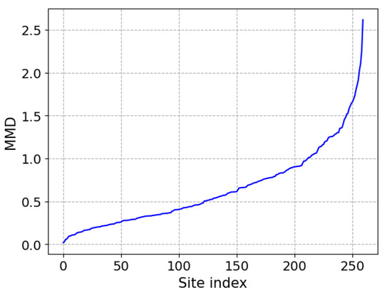
Figure 12.
MMD comparison with VRGAE for different sites. The values of MMD range from 0.02 to 4.69. some similar MMD sites can be clustered according to similar characteristics. Sites near the lowest and maximum values where extreme differences occur were analyzed.
Figure 13 illustrates the Wi-Fi usage pattern of the library’s second floor during the day. Figure 13 shows the Wi-Fi usage expressed as a three-dimensional tensor, such as an image. The shape of the image is horizontal, vertical, and channel, and the shape of the Wi-Fi usage pattern is AP, time, and metric. Because both the image and Wi-Fi usage pattern form a three-dimensional tensor, the Wi-Fi usage pattern can be expressed as an image. One pixel in Figure 13 represents the Wi-Fi usage of AP i at time t. The attributes of Wi-Fi usage are in the form of number of users, RSSI, and throughput, and the image channel is in the form of (R, G, B). It can be interpreted that a pixel close to red implies that only the number of users is high, a pixel close to green indicates the RSSI is high, and a pixel close to blue implies that only the throughput is high. A pixel close to black implies that all metrics are close to 0, and a pixel close to white implies all metrics are close to 1. The number of users, RSSI, and throughput differ in scale. All metrics are mapped to values between 0 and 1 by normalization. There are many dark colors from 00:00 to 06:00 in Figure 13, which indicates that the Wi-Fi usage is low in the early morning. Subsequently, there are many bright colors from 15:00 to 24:00, which implies that the Wi-Fi usage is high in the afternoon.
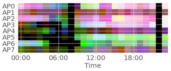
Figure 13.
Wi-Fi usage pattern representation. It represents the Wi-Fi usage pattern of the library’s second floor during the day. One pixel in the figure represents the Wi-Fi usage of AP i at time t.
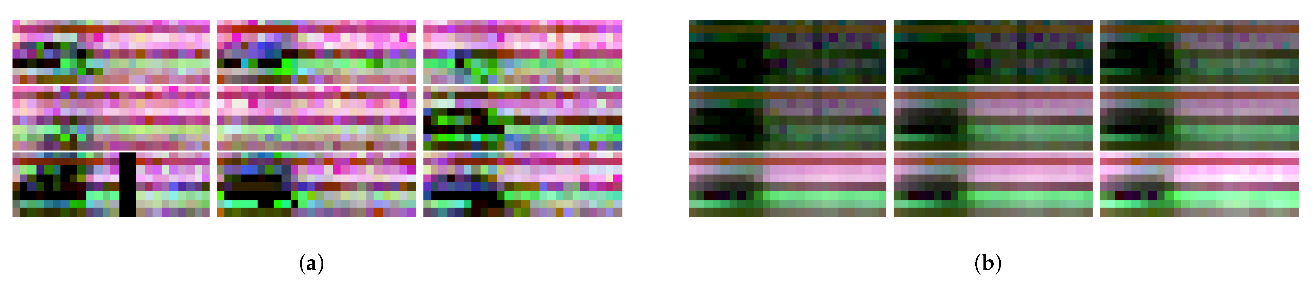
Figure 14 illustrates the Wi-Fi usage patterns over nine days and the sample data from the model. Figure 14a depicts the data on Wi-Fi usage. Not all data show similar patterns but generally record a low usage in the morning and a high usage over time. Some of the data are observed where data are not sampled at rare times. Figure 14b depicts the data sampled from the model. The latent variables z affect the sample. The latent variables, mapped to a normal distribution, create values from −3 to 3 and sample the data. The upper left sample in Figure 14a represents low usage. Moreover, the samples in the lower right are samples with high usage.
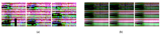
Figure 14.
Wi-Fi usage dataset and sample for 9 days: (a) data, (b) sample. Not all data show similar patterns, but generally record a low usage in the morning and a high usage over time. Samples were also generated by reflecting this usage pattern. The generative model creates an increased usage pattern as the latent variable increases.
The first category of sites were the low MMD sites, which indicated that the distributions of the dataset and sample data were similar. There were 48 sites with an MMD of 0.3 or less. However, there were sites where the Wi-Fi usage itself was shallow. Figure 15 shows the patterns in a site where MMD is close to 0 owing to a very low Wi-Fi usage. First, Figure 15a illustrates a dataset that is mostly black, indicating that values are near-zero in most of the data. Rarely during the day can it be seen that usage occurs at a specific AP. The sample data of Figure 15b are primarily dark and close to zero.
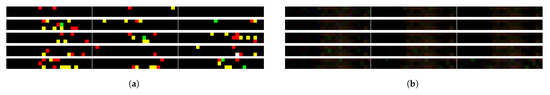
Figure 15.
A site where Wi-Fi is rarely used: (a) data, (b) sample. Among the low MMD sites, there were sites where the Wi-Fi usage was shallow. In (a), the dataset is mostly black, implying that values are near-zero in most of the data. Rarely during the day can it be seen that usage occurs at a specific AP. Samples were also generated by reflecting this usage pattern. Even if the latent variable increases, there is no significant change in the usage patterns.
To confirm that Wi-Fi usage was high or low, all data from each site were averaged and the results were compared. Figure 16 shows the average and MMD of each site. In order to analyze sites representing clear features, the sites with extreme values were studied. There were 10 sites with an average of 0.1 or less. Among the 10 sites, there were 8 sites with an MMD of 0.4 or less again, and 2 sites with an MMD of 6 or more. There were eight sites with an average of 0.4 or more.
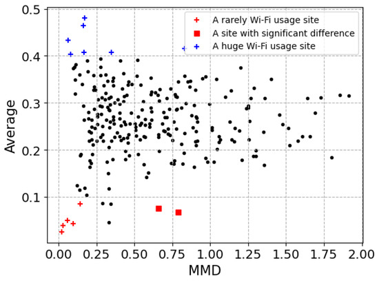
Figure 16.
Scatter plot for each site. This figure represents the average and MMD for each site. A low average means that the overall usage is low. Three characteristic sites are classified through a combination of MMD and data means. Three categories are clustered: sites where Wi-Fi is rarely used, sites with a large difference in Wi-Fi usage on weekdays and weekends, and busy sites.
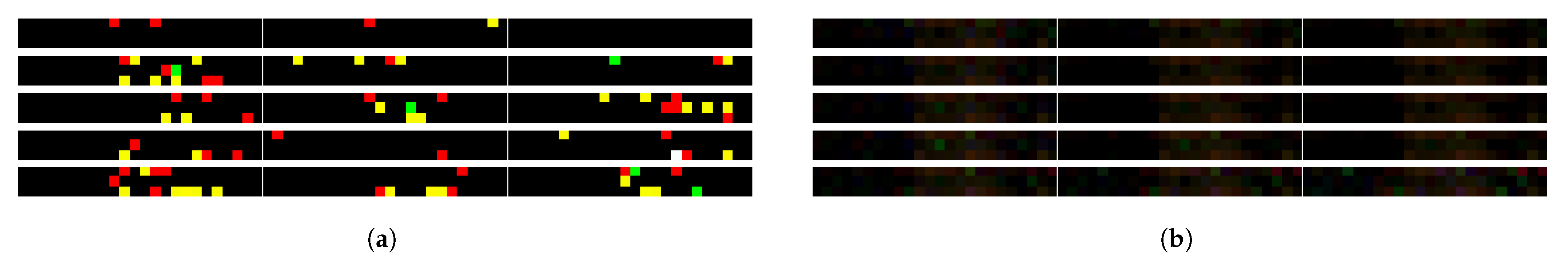
Figure 17 shows the patterns of a site with a significant distribution difference between weekdays and weekends. This site was one of the sites where the data average was less than 0.1 and the MMD value was 0.6 or higher. Figure 17a presents a dataset with weekday data in the first row and weekend data in the second row. Unlike the weekend data, the weekday data are primarily bright. Figure 17b demonstrates the data sampled from the model by adjusting the latent variables. The sampled data differ significantly as Wi-Fi usage patterns vary between weekdays and weekends. The top left figure is the sample output when the value of the latent variable wwas −3. The bottom right figure is the sample output when the value of the latent variable was 3; as the value increases, the Wi-Fi usage increases.
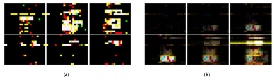
Figure 17.
A site with a large difference in Wi-Fi usage on weekdays and weekends: (a) data, (b) sample. In (a), the first row shows data during a weekday and the second row shows data during a weekend. Unlike the weekend data, the weekday data are primarily bright. Samples were also generated reflecting this usage pattern. The generative model creates an increased usage pattern as the latent variable increases.
Figure 18 shows a very high Wi-Fi usage site. This site had an average of 0.4 or higher. Figure 18a illustrates a dataset and shows bright colors for the majority of the data except at dawn. It implies that all the APs recorded a high usage except at dawn. Figure 18b presents the data sampled from the model by adjusting the latent variables. Just as Wi-Fi usage appeared high on all days, the difference in the sample data was not significant. The top left figure is the sample output when the value of the latent variable was −3. The bottom right figure is the sample output when the value of the latent variable was 3. As the value increases, the difference is not greater than in Figure 17.
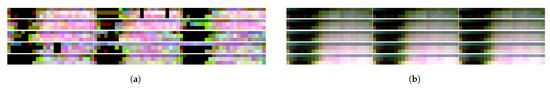
Figure 18.
A busy Wi-Fi site: (a) Data, (b) Sample. (a) shows bright colors for majority of the data except at dawn. Samples were also generated reflecting this usage pattern. The generative model creates an increased usage pattern as the latent variable increases.
5. Discussion
This study modeled the traffic demand of Wi-Fi systems. Traffic demand modeling allows administrators of Wi-Fi systems to solve the problem of relocating APs and allocating radio resources to consider user demand. However, previous studies performed homogeneous modeling of the traffic needs of the users. Traffic modeling is based on statistical models and models spatiotemporal characteristics mathematically. However, spatiotemporal modeling involves a strict assumption in regard to the patterns. Therefore, all traffic patterns follow the assumption of a uniform traffic. This study replaced the existing mathematical modeling that includes a strict assumption with deep learning-based generative models. This generative model ensured that the network traffic demand was heterogeneous.
Previous studies that applied deep learning to networks have focused on traffic prediction problems [13,14,15,16,17,18,19,20,21]. This study attempted to apply deep learning for traffic modeling; however, prediction models are difficult to use. Network traffic modeling, which generates traffic for specific conditions, differs from prediction models in that it requires the information of the previous n steps. Traffic prediction model is a many-to-one mapping. The generative model, which is one-to-many mapping, is suitable for traffic modeling. However, it is rare for generative models to be applied to traffic modeling. There have only been a few intrusion detection studies [27,28,29] that have used the generative model. From a system management perspective, there exist studies, such as Xiao et al. [30] that infer a QoS or the one by Kakkavas et al. [31] that synthesizes a traffic matrix for network management. The contribution of this study is the application of generative models to traffic modeling.
First, the proposed model lowered the difference between the sample data and the data generated by the model by up to 72.1% compared to that reported in previous studies. The AMMD defines the similarity between the existing data distribution and the sample distribution generated by the model. Performance differences arise from difference in the methods with respect to modeling the spatiotemporal characteristics. Previous studies have uniformized the traffic pattern through a strict assumption based on the data collected from all APs. This assumption assigns identical traffic patterns to a restaurant with traffic characteristics concentrated at lunchtime and to an office that exhibits high traffic at work time. However, this study modeled the spatiotemporal characteristics of individual APs by learning traffic patterns for each AP. Thus, the proposed model enabled a more detailed modeling of the spatiotemporal characteristics at the AP level.
Second, this study confirmed a difference in performance depending on the structure of the model. Deep learning models have devised components to reflect each characteristic and learn spatiotemporal patterns. The components used in this study were the GRU that considered the temporal characteristics and the GC that considered the spatial characteristics. The results showed a higher performance when the model utilized the GRU and GC.
Finally, this study evaluated the performance of different sites. The traffic patterns appearing at each site were investigated to determine the difference in the performance of the models. Accordingly, an AMMD difference from 0.02 to 4.69 was observed. The MMD represents the difference between existing data and samples generated by the model, but this value need not simply be high or low in order to determine the success of the learning task. For example, among the sites with a low MMD, there was a site in which all metrics were recorded as zero. This implied that in that site, none of the APs were used. Consequently, the model appeared to be satisfactory; however, there was nothing to learn about the pattern. In addition, among the spaces with a high MMD, there were sites with a vast difference between weekdays and weekends. These sites exhibited a large difference in traffic at time t during the learning process, resulting in poor results.
6. Conclusions
This study proposed a generative model for Wi-Fi traffic demand. The proposed model generated Wi-Fi traffic patterns for system-level network simulations. Measurement data were collected from the APs established at PNU. An analysis of the data verified that the Wi-Fi traffic displayed an iterative pattern in daily intervals, and APs at the same site recorded different traffic demands. The results from the data analysis indicated the necessity for a more sophisticated modeling incorporating both time and spatial factors when portraying traffic demand. Therefore, this study divided the total Wi-Fi service area into each floor level, which was one spatial unit, and that spatial unit depicted the correlation between Wi-Fi usage through an interference matrix between the APs. The generative model for the Wi-Fi traffic demand considered the spatiotemporal characteristics. The spatial and temporal characteristics were modeled with the GC and GRU, respectively.
This study evaluated the similarity of the samples generated from models with a dataset. There were three performance evaluation. The first evaluation compared the distribution between the existing and proposed models. The second evaluation compared the distributions between the sample data generated from the proposed models and the dataset, thus comparing the performance of the proposed models. The third evaluation compared the distributions between the sample data and the dataset for each site. It classified sites according to the performance of the generative models and analyzed traffic patterns at each site.
Generative models are readily available. Network managers can collect data and model Wi-Fi user demand. Data collection, such as metrics at the AP level, can be collected from the controller. It can save the effort of finding a traffic model for each AP. As mentioned earlier, APs at the site have different traffic patterns. Applying an appropriate traffic model for each AP can take considerable time. Generative models can be solved simply by learning from collected data.
Despite the limitation of this model, such as the constraint that it was used at PNU, the evaluation conducted in this study verified that sites were exhibiting similar spatiotemporal characteristics. However, the data collection for a target site would be required to apply the proposed model to another site. Future research will group the characteristics of the traffic model so that it can be applied directly to other sites.
Author Contributions
Conceptualization, J.-M.L. and J.-D.K.; methodology, J.-M.L.; software, J.-M.L.; validation, J.-M.L. and J.-D.K.; formal analysis, J.-M.L.; investigation, J.-M.L.; resources, J.-M.L.; data curation, J.-M.L.; writing—original draft preparation, J.-M.L.; writing—review and editing, J.-M.L. and J.-D.K.; visualization, J.-M.L.; supervision, J.-D.K.; project administration, J.-D.K.; funding acquisition, J.-D.K. All authors have read and agreed to the published version of the manuscript.
Funding
This research was supported by the MSIT (Ministry of Science and ICT), Korea, under the Grand Information Technology Research Center support program (IITP-2022-2016-0-00318) supervised by the IITP (Institute for Information & communications Technology Planning & Evaluation) and this research was supported by Basic Science Research Program through the National Research Foundation of Korea (NRF) funded by the Ministry of Education (NRF-2020R1I1A3065947).
Data Availability Statement
The data are not publicly available due to security concerns.
Conflicts of Interest
The authors declare no conflict of interest.
References
- Rahman, M.A.; Pakštas, A.; Wang, F.Z. Network modelling and simulation tools. Simul. Model. Pract. Theory 2009, 17, 1011–1031. [Google Scholar] [CrossRef] [Green Version]
- Chandrasekaran, B. Survey of network traffic models. Waschington Univ. St. Louis CSE 2009, 567, 1–8. [Google Scholar]
- Hernández-Campos, F.; Karaliopoulos, M.; Papadopouli, M.; Shen, H. Spatio-temporal modeling of traffic workload in a campus WLAN. In Proceedings of the 2nd Annual International Workshop on Wireless Internet, Boston, MA, USA, 2 August 2006. [Google Scholar]
- Ghosh, A.; Jana, R.; Ramaswami, V.; Rowland, J.; Shankaranarayanan, N.K. Modeling and characterization of large-scale Wi-Fi traffic in public hot-spots. In Proceedings of the 2011 Proceedings IEEE INFOCOM, Shanghai, China, 10 April 2011. [Google Scholar]
- Wu, B.; Nair, S.; Martin-Martin, R.; Fei-Fei, L.; Finn, C. Greedy hierarchical variational autoencoders for large-scale video prediction. In Proceedings of the IEEE/CVF Conference on Computer Vision and Pattern Recognition, Nashville, TN, USA, 25 June 2021. [Google Scholar]
- Saito, S.; Hu, L.; Ma, C.; Ibayashi, H.; Luo, L.; Li, H. 3D hair synthesis using volumetric variational autoencoders. ACM Trans. Graph. TOG 2018, 37, 1–12. [Google Scholar] [CrossRef]
- El-Kaddoury, M.; Mahmoudi, A.; Himmi, M.M. Deep generative models for image generation: A practical comparison between variational autoencoders and generative adversarial networks. In Proceedings of the International Conference on Mobile, Secure, and Programmable Networking, Mohammedia, Morocco, 28 October 2019. [Google Scholar]
- Chen, Y.C.; Kurose, J.; Towsley, D. A mixed queueing network model of mobility in a campus wireless network. In Proceedings of the 2012 Proceedings IEEE INFOCOM, Orlando, FL, USA, 25 March 2012. [Google Scholar]
- Ding, J.; Xu, R.; Li, Y.; Hui, P.; Jin, D. Measurement-driven modeling for connection density and traffic distribution in large-scale urban mobile networks. IEEE Trans. Mob. Comput. 2017, 17, 1105–1118. [Google Scholar] [CrossRef]
- Marvi, M.; Aijaz, A.; Khurram, M. Integrating Stochastic Geometry and ON/OFF Traffic Models: Toward Spatio-Temporal Analysis of Wireless Networks With Heterogeneous Services. IEEE Trans. Netw. Sci. Eng. 2022, 9, 1668–1679. [Google Scholar] [CrossRef]
- Wang, G.; Zhong, Y.; Li, R.; Ge, X.; Quek, T.Q.S.; Mao, G. Effect of Spatial and Temporal Traffic Statistics on the Performance of Wireless Networks. IEEE Trans. Commun. 2020, 68, 7083–7097. [Google Scholar] [CrossRef]
- Zhang, C.; Ouyang, X.; Patras, P. ZipNet-GAN: Inferring fine-grained mobile traffic patterns via a generative adversarial neural network. In Proceedings of the 13th International Conference on Emerging Networking EXperiments and Technologies, Incheon, Korea, 12–15 December 2017; pp. 363–375. [Google Scholar]
- Wang, J.; Tang, J.; Xu, Z.; Wang, Y.; Xue, G.; Zhang, X.; Yang, D. Spatiotemporal modeling and prediction in cellular networks: A big data enabled deep learning approach. In Proceedings of the IEEE INFOCOM 2017-IEEE Conference on Computer Communications, Atlanta, GA, USA, 1 May 2017. [Google Scholar]
- He, K.; Chen, X.; Wu, Q.; Yu, S.; Zhou, Z. Graph Attention Spatial-Temporal Network With Collaborative Global-Local Learning for Citywide Mobile Traffic Prediction. IEEE Trans. Mob. Comput. 2022, 21, 1244–1256. [Google Scholar] [CrossRef]
- Fang, L.; Cheng, X.; Wang, H.; Yang, L. Mobile demand forecasting via deep graph-sequence spatiotemporal modeling in cellular networks. IEEE Internet Things J. 2018, 5, 3091–3101. [Google Scholar] [CrossRef]
- Zhang, C.; Patras, P. Long-term mobile traffic forecasting using deep spatio-temporal neural networks. In Proceedings of the Proceedings of the Eighteenth ACM International Symposium on Mobile Ad Hoc Networking and Computing, Los Angeles, CA, USA, 25 June 2018. [Google Scholar]
- Zhang, C.; Zhang, H.; Qiao, J.; Yuan, D.; Zhang, M. Deep Transfer Learning for Intelligent Cellular Traffic Prediction Based on Cross-Domain Big Data. IEEE J. Sel. Areas Commun. 2019, 37, 1389–1401. [Google Scholar] [CrossRef]
- Wang, X.; Zhou, Z.; Xiao, F.; Xing, K.; Yang, Z.; Liu, Y.; Peng, C. Spatio-Temporal Analysis and Prediction of Cellular Traffic in Metropolis. IEEE Trans. Mob. Comput. 2019, 18, 2190–2202. [Google Scholar] [CrossRef] [Green Version]
- Zhang, C.; Zhang, H.; Yuan, D.; Zhang, M. Citywide Cellular Traffic Prediction Based on Densely Connected Convolutional Neural Networks. IEEE Commun. Lett. 2018, 22, 1656–1659. [Google Scholar] [CrossRef]
- Trinh, H.D.; Giupponi, L.; Dini, P. Mobile Traffic Prediction from Raw Data Using LSTM Networks. In Proceedings of the 2018 IEEE 29th Annual International Symposium on Personal, Indoor and Mobile Radio Communications (PIMRC), Bologna, Italy, 9 September 2018. [Google Scholar]
- Feng, J.; Chen, X.; Gao, R.; Zeng, M.; Li, Y. DeepTP: An End-to-End Neural Network for Mobile Cellular Traffic Prediction. IEEE Netw. 2018, 32, 108–115. [Google Scholar] [CrossRef]
- Kim, H.W.; Lee, J.H.; Choi, Y.H.; Chung, Y.U.; Lee, H. Dynamic bandwidth provisioning using ARIMA-based traffic forecasting for mobile WiMAX. Comput. Commun. 2011, 34, 99–106. [Google Scholar] [CrossRef]
- Zhang, S.; Tong, H.; Xu, J.; Maciejewski, R. Graph convolutional networks: A comprehensive review. Comput. Soc. Netw. 2019, 6, 1–23. [Google Scholar] [CrossRef] [Green Version]
- Rusek, K.; Suárez-Varela, J.; Almasan, P.; Barlet-Ros, P.; Cabellos-Aparicio, A. RouteNet: Leveraging Graph Neural Networks for network modeling and optimization in SDN. IEEE J. Sel. Areas Commun. 2020, 38, 2260–2270. [Google Scholar] [CrossRef]
- Li, J.; Sun, P.; Hu, Y. Traffic modeling and optimization in datacenters with graph neural network. Comput. Netw. 2020, 181, 107528. [Google Scholar] [CrossRef]
- Sone, S.P.; Lehtomäki, J.J.; Khan, Z. Wireless traffic usage forecasting using real enterprise network data: Analysis and methods. IEEE Open J. Commun. Soc. 2020, 1, 777–797. [Google Scholar] [CrossRef]
- Shahid, M.R.; Blanc, G.; Jmila, H.; Zhang, Z.; Debar, H. Generative Deep Learning for Internet of Things Network Traffic Generation. In Proceedings of the 2020 IEEE 25th Pacific Rim International Symposium on Dependable Computing (PRDC), Perth, Australia, 1 December 2020. [Google Scholar]
- Ring, M.; Schlör, D.; Landes, D.; Hotho, A. Flow-based network traffic generation using Generative Adversarial Networks. Comput. Secur. 2019, 82, 156–172. [Google Scholar] [CrossRef] [Green Version]
- Lin, Z.; Shi, Y.; Xue, Z. IDSGAN: Generative Adversarial Networks for Attack Generation Against Intrusion Detection. arXiv 2018, arXiv:1809.02077. [Google Scholar]
- Xiao, S.; He, D.; Gong, Z. Deep-Q: Traffic-Driven QoS Inference Using Deep Generative Network. In Proceedings of the 2018 Workshop on Network Meets AI & ML, Budapest, Hungary, 19 August 2018. [Google Scholar]
- Kakkavas, G.; Kalntis, M.; Karyotis, V.; Papavassiliou, S. Future Network Traffic Matrix Synthesis and Estimation Based on Deep Generative Models. In Proceedings of the 2021 International Conference on Computer Communications and Networks (ICCCN), Athens, Greece, 19 July 2021. [Google Scholar]
- Sohn, K.; Lee, H.; Yan, X. Learning structured output representation using deep conditional generative models. Adv. Neural Inf. Process. Syst. 2015, 28, 3483–3491. [Google Scholar]
- Goodfellow, I.; Pouget-Abadie, J.; Mirza, M.; Xu, B.; Warde-Farley, D.; Ozair, S.; Courville, A.; Bengio, Y. Generative adversarial nets. Adv. Neural Inf. Process. Syst. 2014, 27, 2672–2680. [Google Scholar]
- Adame, T.; Carrascosa, M.; Bellalta, B. The TMB path loss model for 5 GHz indoor WiFi scenarios: On the empirical relationship between RSSI, MCS, and spatial streams. In Proceedings of the 2019 Wireless Days, Manchester, UK, 24 April 2019. [Google Scholar]
- Drieberg, M.; Zheng, F.C.; Ahmad, R.; Fitch, M. Impact of interference on throughput in dense WLANs with multiple APs. In Proceedings of the 2009 IEEE 20th International Symposium on Personal, Indoor and Mobile Radio Communications, Tokyo, Japan, 13 September 2009. [Google Scholar]
- Kipf, T.N.; Welling, M. Semi-supervised classification with graph convolutional networks. In Proceedings of the International Conference on Learning Representations 2016, San Juan, Puerto Rico, 2 May 2016. [Google Scholar]
- LeCun, Y.; Bengio, Y.; Hinton, G. Deep learning. Nature 2015, 521, 436–444. [Google Scholar] [CrossRef] [PubMed]
- Kolen, F.; Kremer, C. Gradient Flow in Recurrent Nets: The Difficulty of Learning Long-Term Dependencies. In A Field Guide to Dynamical Recurrent Networks; Wiley-IEEE Press: Piscataway, NJ, USA, 2001; pp. 237–243. [Google Scholar]
- Gers, F.A.; Schmidhuber, J.; Cummins, F. Learning to forget: Continual prediction with LSTM. Neural Comput. 2000, 12, 2451–2471. [Google Scholar] [CrossRef] [PubMed]
- Cho, K.; Van Merriënboer, B.; Gulcehre, C.; Bahdanau, D.; Bougares, F.; Schwenk, H.; Bengio, Y. Learning phrase representations using RNN encoder-decoder for statistical machine translation. arXiv 2014, arXiv:1406.1078. [Google Scholar]
- Ravanelli, M.; Brakel, P.; Omologo, M.; Bengio, Y. Light gated recurrent units for speech recognition. IEEE Trans. Emerg. Top. Comput. Intell. 2018, 2, 92–102. [Google Scholar] [CrossRef] [Green Version]
- IT Center in Pusan National University. Available online: https://uitc.pusan.ac.kr/ (accessed on 9 May 2022).
- Gretton, A.; Borgwardt, K.; Rasch, M.; Schölkopf, B.; Smola, A. A kernel method for the two-sample-problem. Adv. Neural Inf. Process. Syst. 2006, 19. [Google Scholar]


Publisher’s Note: MDPI stays neutral with regard to jurisdictional claims in published maps and institutional affiliations. |
© 2022 by the authors. Licensee MDPI, Basel, Switzerland. This article is an open access article distributed under the terms and conditions of the Creative Commons Attribution (CC BY) license (https://creativecommons.org/licenses/by/4.0/).