1. Introduction
In 2020, the world’s energy derived from photovoltaic sources (PVs) exceeded 3.1% of the total world energy generation with a 23% growth compared to 2019. It is currently the third major source of renewable energy behind hydropower and off-shore wind generation [
1].
Renewable energy sources are subject to volatile weather conditions, thus presenting a major challenge. For instance, the energy drop in actual PV energy generation compared to forecast energy can be as high as 20% [
2] while the associated costs with errors in wind power forecasts can be as high as 10% as estimated in [
3] for the Spanish market.
Cloud dynamics play an important role in predicting PV energy output which in turn is directly linked to the solar radiation reaching the farm. According to [
4] it has been estimated that if all clouds were to be removed, the absorbed solar radiation would increase by about 50
. In fact, it has been shown that clouds represent the most significant source of error in the extraction of earth surface energy and water balance parameters out of meteorological satellite data, with other measurable factors such as the concentration of aerosols having a secondary impact [
5].
Forecast horizons ranging from 24 h to 72 h ahead are important for power grids partially fed by PV parks. However, three categories of short-time forecasts for PV energy production are of major interest [
6]:
intra-hour: time horizons ranging from minutes to one hour;
nowcasting (up to two-hours ahead) of high-frequency variability in electricity production targeting real-time control of the grid equilibrium, technical constraints related to start-up times of conventional power sources connected to the grid as balancing instruments;
intra-day: hourly sampling with a maximum look-ahead time of six hours, targeted to follow the forecast demand, such forecasts also being useful for hourly trading market;
day ahead: at hourly sampling, aiming to meet needs in planning the production of controlled fossil fuel plants and also useful for PV owners for accessing the Day Ahead Market (DAM) of electricity.
Depending on the spatio-temporal scale of the application, irradiance can be predicted up to 30 min ahead at a single site using all-sky imagers, up to six h ahead using satellite images or satellite-derived irradiance, or several days ahead using numerical weather prediction (NWP) [
7,
8]. In fact, research has shown that for nowcasting, image-based methods outperform numerical methods [
9].
However, accessing high-quality forecasts is not easy, as evidenced by PV farm operators who change forecast supplies regularly in an attempt to reduce their profit losses. In Romania for instance, operators have changed on average 20 suppliers over the last five years, according to the Romanian Sustainable Energy Cluster. This drives the need for personalized on-demand forecasts accessible to regular PV farm operators. The problem is that running NWP simulations in addition to high-frequency multi-spectral image analysis requires resources and time [
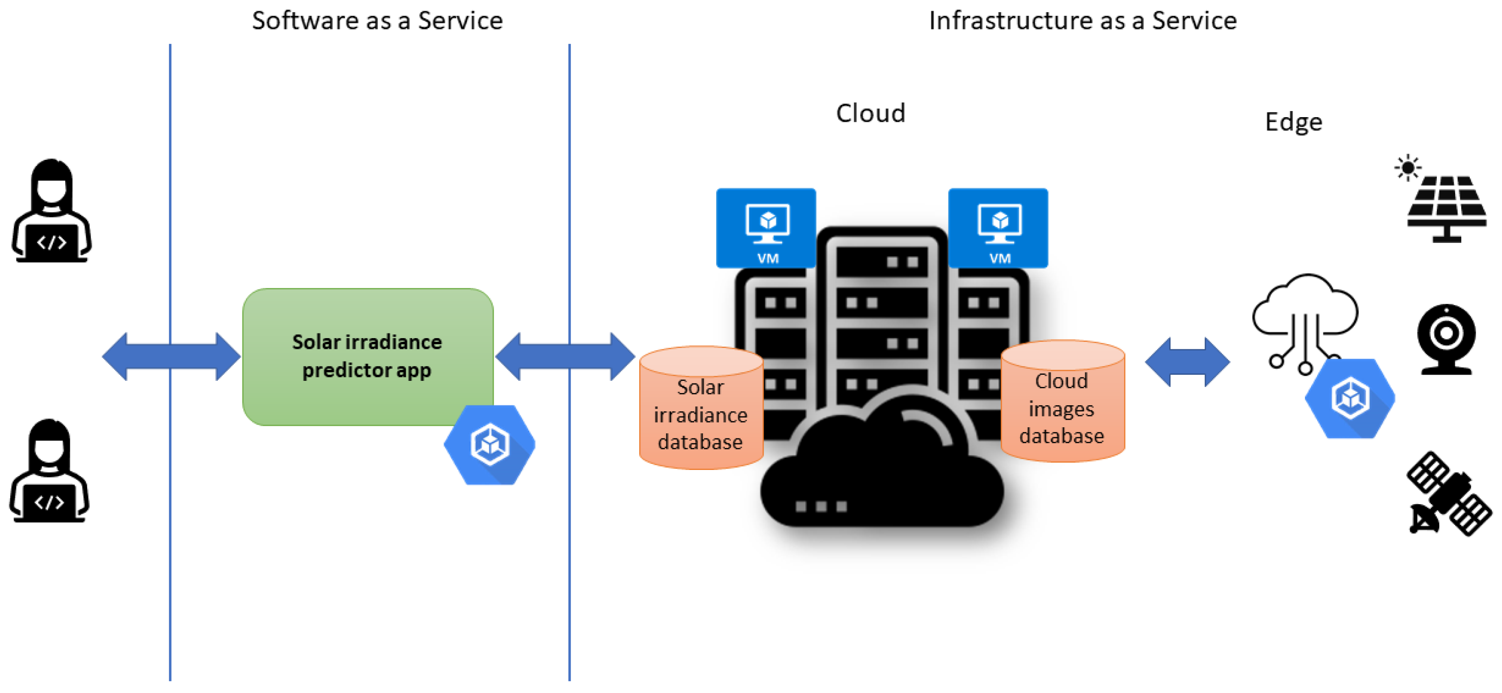
10], rendering these tasks unfeasible on commodity machines. In addition, these custom-tailored solutions require specialized IT knowledge which incurs additional costs to PV operators. However, the increased accessibility of multicore and manycore solutions with faster processing times enable PV operators to run these models closer to their PV infrastructure by Software as a Service (SaaS) solutions (1) employing low latency edge computing for vital real-time tasks such as intra-hour or nowcasting forecasting with less constrained operations, and (2) higher latency remote clouds for intra-day or day ahead planning. Combined with simpler yet accurate models for cloud dynamics and irradiance these methods can enable PV operators access to fast and reliable PV energy output forecasts.
In this paper, we propose an SaaS container-based solar platform capable of automatically deciding the optimal location to perform the forecast, on edge (near the PV farm) or remotely in the cloud. We show that two important components in the PV output forecast, namely cloud dynamics prediction and irradiance levels can be accurately determined for nowcasting using simple methods. Specifically, our objectives are:
A novel scalable forecast of cloud dynamics based on satellite and all-sky imagery by employing a nature-inspired algorithm suitable for now-casting and intra-day predictions [
11,
12] using openly available datasets;
Investigation on the real-life feasibility of determining cloud type based on several sources such as multispectral information extracted from weather satellites (e.g., GOES, Meteosat); and
A new method based on statistics and machine learning to forecast solar irradiance for a given site based on historical correlation between cloudy pixel value and measured irradiance (performed a priori by a nearby solar monitoring station).
The paper extends our previous work on the cloud dynamics forecast [
11,
12,
13]. Specifically, in this article we introduce the edge–cloud continuum platform and the irradiance forecast method.
The rest of the paper is structured as follows:
Section 2 gives an overview on existing cloud- and edge-based solutions for PV monitoring and analysis as well as on algorithms for cloud dynamics and irradiance forecast.
Section 3 introduces the proposed cloud–edge architecture and proof-of-concept component-based platform, including the modules for cloud dynamics, cloud type, and irradiance forecast.
Section 4 presents some experimental results in terms of scalability and accuracy. Finally,
Section 5 outlines the main conclusions and future work.
3. Proposed Architecture
The last decade has seen a surge in the computational capabilities of devices lying at the edge of the network. Previously, the computational power was concentrated in big data centres, possessing high bandwidth and inter-connectivity. With the advent of IoT and the prospect of smart technologies, research and industry alike are investing money and effort in designing more capable edge devices, high bandwidth connections, and platforms that will handle the data processing workflows on the cloud–edge continuum.
Figure 1 shows our vision of such a layered architecture targeting solar irradiance predictions.
Kubernetes [
37] is a popular resource management platform, allowing users to scale and automate container applications. The majority of Cloud providers offering container deployments also offer the possibility to create Kubernetes clusters to manage application elasticity. Recently, a lightweight (
https://k3s.io/, accessed on 22 August 2022) version of the Kubernetes platform was designed for IoT devices. A preliminary study [
38] has shown it has a great advantage with respect to disk, memory, and CPU utilization, as well as time required for different procedures (e.g., add worker, start deployment).
Our proposed architecture enabling hybrid cloud–edge deployment is presented in
Figure 2 and consists of several components. The end-user interested in solar radiation prediction will interact with our SaaS solution through a web user interface. Similarly, programmers can access the platform through a REST API. Users will select a geographical region of interest, a prediction window, and the type of data to use. The core of our platform consists of two components: service and data orchestrators. The Service Orchestrator interprets the user request and identifies a set of operations to be carried out. The platform maintains descriptions for the offered services. A service (deployed as a container) is described by some requirements (CPU, memory, GPU), the input/output data types, and a Docker Image (initially stored on Docker Hub, but cached by nodes running the images). Examples of services include our core modules: Cloud Dynamics forecast CPU/GPU enabled, Cloud Detection, and Irradiance prediction.
The Data Orchestrator component maintains a record of data locations. In the beginning, the data locations are initiated with public data servers containing satellite images and irradiance historical data. As services run and data are transferred, the system will prefer to run subsequent applications near the new location for the data.
The Service Orchestrator uses the data location information to select a set of services that need to be run to achieve the desired result. For example, if cloud masks have been generated by a previous user request and have been stored in a storage bucket or FTP server, then the Cloud Detection/Dynamics services do not need to be executed again. Moreover, if cloud masks have already been predicted for a region and they are still valid (i.e., the interval where the accuracy of the model is under a predetermined threshold) they can be reused by the irradiance prediction service. In general, this component will create a workflow consisting of a Directed Acyclic Graph (DAG) where nodes represent the services and edges represent data dependencies between services.
The Service Orchestrator will ask one or more Cloud and Edge Scheduling components to find resources for running the services, providing back a solution. For the Cloud Dynamics service, our platform offers two implementations: a CPU and a GPU version. In this case, the GPU version will be preferred. If there are no free GPUs for the scheduler, then a workflow with the CPU version is requested.
A Cloud Scheduler manages a Kubernetes cluster within a cloud region. A Regional Scheduler manages one or more Kubernetes clusters that are close from a network point of view. The Service Orchestrator has knowledge of multiple Regional and Cloud schedulers from which it can choose the best deployment for a workflow.
3.1. Example Workflow
In this example, we consider the system in its initial state, with no service or data transfer history. When the first user requests an irradiance prediction for a geographical region, the workflow presented in
Figure 3 will be generated by the Service Orchestrator service. First, satellite images need to be made available to the Cloud Detection service using a storage service. This service will generate cloud masks from the recent satellite images. The cloud masks will be used by the Cloud Dynamics service to compute the optical flow and predict the motion of the identified clouds. This will create new cloud masks representing where the clouds will appear in the future. Finally, the Irradiance Prediction service will use the predicted cloud masks and historical irradiance data to forecast the new values.
The cloud mask data will be persisted in Cloud Storage buckets to be reused by subsequent runs of the Cloud Dynamics Service. Predicted cloud masks are also cached given that they are valid; when the satellite image database is updated, a new mask has to be generated to replace the predicted one. Finally, predicted irradiance will also be stored short-term, similar to predicted cloud masks.
We assume that generic users are interested in small regions under 100 . While the Irradiance Prediction service can work with data relevant for this small region, the Cloud Dynamics service requires a larger area to increase the accuracy of the predicted motion. Therefore, cloud masks can be generated for larger areas (i.e., countries, continents) and used by multiple irradiance prediction services, each interested in a smaller area contained within the cloud mask.
In order to provide the functionalities described in
Section 3, the scheduler needs to be aware not only of the state of the data, but also of the hardware features and availability of each node. A service may depend on or prefer several features such as number of cores, amount of memory, disk space, or GPU cards.
Computing nodes must be selected so as to minimize data movement for the entire workflow of the application. In our approach we deploy the services as close to the data as possible. However, nodes in a Kubernetes cluster will use data from a location which may be external to the node, mounted using a network file system. Therefore, all nodes being part of the same cluster are equal from the data locality point of view.
A prediction job involves the setting of several parameters, defined in
Table 1. Cloud movement predictions work best for GOES-R images which are captured twice per hour. Using at least 100,000 particles the predictions for cloud movement show an F1-score in the interval of
for the first 5 h. More details on the impact of these parameters are presented in [
11].
3.2. Datasets
Given the different properties and availability of free data sources the proposed platform supports different formats (e.g., satellite, all-sky camera). Traditional cloud-type inference algorithms rely on multispectral images from satellites, but short-term forecasts usually employ all-sky RGB cameras as multispectral images at such a frequency are usually not freely available. In
Table 2 we have listed the characteristics of each Sentinel 2 band and the closest wavelength-wise correspondents from Meteosat SEVIRI and NOAA GOES-R. Ideally, each module will process the same dataset, but some data benefit a module more than the other.
The Cloud Dynamics module was tested and works best on images from geostationary satellites because they are locked to the rotation of the Earth and capture images every 15 min to 30 min. The images from these satellites are especially suitable for detecting cloud movement and forecasting cloud position. The downside, however, is that rotation-locked satellites operate at very high altitudes and the produced images have low spatial resolutions, negatively impacting the forecast precision in terms of extent. Results are good for large regions, but they are not granular enough to be useful on lower scales such as street- or neighborhood-wide forecasts. In addition, freely available datasets are not multispectral rendering them unsuitable for inferring cloud types (
Section 3.4).
The Cloud (type) Detection module was tested on images from the orbiting Sentinel 2 satellite. Its onboard sensors have a higher spatial resolution (approx. 10 m/pixel) enabling precise isolation of cloudy pixels from land and water. Clouds can be separated by type and ground-measured irradiance data can be correlated with clouds that are directly on top of the irradiance sensor. Not being locked to the rotation of the Earth means that Sentinel has its orbit and is much closer to the ground than geostationary satellites. The downside is that it takes 2–3 days for the satellite to pass over the same geographic region, so there is a trade-off between higher resolution images and higher frequency captures: one is good for precise detection of cloud types and correlating with irradiance at large intervals, the other is better for forecasting cloud dynamics.
For testing this module we used the following datasets:
Imagery from NOAA Goes satellite. The color composite images from this geostationary satellite include North America and are captured at 30 intervals. The dynamics module was tested on 1920 × 1080 pixel images from 2017 onward.
Imagery from Sentinel 2. The orbiting satellites provide imagery in 13 reflectivity bands (see
Table 2) at 10, 20, and 60 m spatial resolutions. We used imagery that captured western Romania, which includes the city of Timisoara where the solar platform providing our irradiance data is installed. Images were retrieved for the years 2020 and 2021. Sentinel images are squares with a width of 10,980 pixels.
Irradiance from a solar platform. The West University of Timisoara (UVT) has a solar radiation station that measures irradiance among other metrics. We retrieved GI and DI in days where Sentinel imagery was also available.
The modules were tested on different datasets due to the trade-off between time and spatial resolutions. Geostationary satellites have dense temporal resolution, but lack the spatial resolution of low orbit satellites. Next, we detail each module (since they are exposed as services we will use the terms interchangeably).
3.3. Cloud Dynamics Module
The module responsible for detecting and forecasting motion uses the optical flow technique proposed by Farnebäck [
19] and a modified version of the flocking behavior meta-heuristics developed by Reynolds [
39] to simulate the synchronous movement of animal groups.
Figure 4 illustrates the three main stages of the cloud motion forecast.
The module requires a series of sequential satellite images. It then proceeds by analyzing all sequential pairs using optical flow and generates a
master flow from the resulting set of displacement fields [
13]. The master flow is an average of the movement detected in the scene, so we consider it to be similar to a wind map of the scene as cloud motion is driven by windand clouds are the only moving object in the scene. Changes caused by humans are not visible. For instance, geostationary weather satellites capture images of the same geographical regions every 15 min to 30 min and surface land or water features are constant. Events such as urbanization or deforestation are visible in larger time scales, so they do not impact the movement detection of clouds.
After the wind map is generated, the service overlaps a layer of “cloud particles” arranged according to a mask of the last known clouds’ position. The mask is initially inferred from the displacement field of the last motion detection, based on the above-mentioned movement arguments. However, the Cloud Detection module can also be used to generate a mask for this step. A benefit of doing so is that we obtain opacity data alongside cloud position. This, in turn, helps for better forecast and cloud form visualization. The cloud particle layer exists in the same space as the wind map, i.e., each particle is positioned directly on top of a motion vector.
Finally, the module applies the modified version of the flocking algorithm on the wind map to simulate movement and forecast cloud position. The algorithm uses rules that update each motion vector in the wind map according to its surroundings and takes into consideration real-world wind behavior. A detailed explanation as well as a discussion on its accuracy is provided in [
12]. A motion vector is affected by neighbors that move towards it and will change the direction of motion to match its neighbors’. To mimic wind, motion vectors forming a curved path will be nudged outwards by lessening the turning degree magnitude. The application of the rules to the entire wind map generates a new wind map which then affects the layer of cloud particles by essentially carrying each “cloud particle” according to its corresponding motion vector. The updated cloud particle layer represents the forecast cloud position. Repeated and continuous application of the rules on the wind map and updating of the cloud layer output multiple forecasts that follow each other. The time interval between the forecasts is equal to the image frequency, i.e., 15 min to 30 min.
The proposed model can be applied in the real world with medium to high precision for the first 5 h of forecast (
Section 3.1 and
Section 4.1, and [
11]). Our proposed model is advantageous because it can simulate non-linear cloud particle dynamics. The drawbacks of this model are related to condensation and evaporation, which are not taken into account in the current version.
3.4. Cloud Detection Module
Clouds can be detected and their types determined from multispectral images [
29]. These are openly available (to a varying degree) both from Earth Observation (EO) satellites (e.g., Sentinel 2) and from geostationary weather satellites (e.g., Meteosat, NOAA GOES). Usually a combination of red, vegetation, and (near) infrared images is used [
40], but some satellites have special bands for high-altitude cirrus clouds. The advantage of EO satellites is spatial resolution (reaching as low as a few meters); however, the frequency of images over a given area is unsuited for PV energy output forecast.
For instance, Sentinel 2 captures images of Earth using 13 bands that were built specifically for different types of remote sensing (
Table 2), Meteosat SEVIRI has 12 bands [
41], and NOAA GOES-R has 16 bands [
42].
In what follows we rely on Sentinel 2 naming from
Table 2 for clarity. Since it has been shown that thresholding values depend on the region (e.g., water, land, ice) [
43] we present next an algorithm working over land as PV farms which interest us are placed on soil.
To identify the types of cloud in an image, we use a thresholding method that combines information from four Sentinel 2 bands: the red band (B04), the near-infrared band (B08), the water vapor band (B09), and the cirrus band (B10). It can be seen that not all these bands are present in geostationary satellites with some offering close approximations. This makes it challenging in using these images to extract cloud types but they can be used for cloud masks as shown in
Section 3.3. Before proceeding we note that some cloud types (e.g., cirrus, low stratus, roll cumulus) are difficult to detect because of insufficient contrast with the surface radiance [
43]. Our aim is to detect three types of clouds: thick convective clouds (cumulonimbus), low clouds (fog, stratus), and thin high clouds (cirrus). The choice of cloud types is motivated by the published work of Menzel [
44], in which he details best practices to identify clouds using multiple wavelength tests. A general algorithm for extracting clouds (from Landsat images) is given in [
45] (and adapted by us to Sentinel 2 bands):
where the values for the B* bands indicate the top-of-atmosphere reflectance.
The module first isolates most clouds by performing a
reflectance ratio test [
43] involving the red (660 nm band—B04) and near-infrared (870 nm band—B08) bands. For each pixel, it computes the ratio between the two bands and tests that it is between 0.9 and 1.1 but could be lowered to as much as 0.8 or 0.75 in some cases:
where
i and
j are the pixel’s coordinates, and
allCloudMask represents the cloud mask. It is common to use the 865 nm vegetation band (B8A) instead of the 842 nm near infrared band (B08), but the latter has a wider bandwidth of 115 nm versus the former’s 20 nm. This means that the two bands overlap and the near infrared band (B08) captures a wider spectrum than the vegetation band (B8A) which can be considered a subset.
Convective as well as stratiform clouds are detected using the near-infrared (B08) and water vapor (B09) bands (the brightness temperature in the water vapor absorption channel is warmer than that in the atmospheric infrared window [
46]):
where
convCloudMask represents the convective cloud mask. Difference tests such as this one are often named split windows techniques and usually involve using 11.000 nm wavelengths and over, but Sentinel 2 has its largest band centered around 2190
thus we use different wavelengths to perform the tests.
Recently, an algorithm relying on red and infrared bands was proposed [
47].
Low altitude clouds (fog, stratus) are identified by removing convective clouds from the initial cloud mask:
where
convCloudMask represents the convective cloud mask.
Another approach is to use B11 band which discriminates low clouds from snow [
48].
The cirrus band (B10) in near infrared is specifically designed for detecting high-thin cirrus so the resulting image is directly used as a mask for cirrus clouds.
Masking is performed for all available images in the time series.
3.5. Irradiance Prediction Module
Finally, the irradiance prediction module computes the correlation between the GI and DI, and the values of the masked cloud types. Since determining the cloud type is a rather challenging and inaccurate (
Section 2 and
Section 3.4) process due to the required parametrization, we also correlate irradiance levels directly with RGB information to verify the predictability of irradiance without a priori knowledge of cloud types as inferring them requires, in most cases, multispectral images not easily accessible by the general public (
Section 3.4. Despite having 13 bands, only some of the wavelengths are sensitive to or interfere in any way with clouds. Therefore, we compute correlations only for specific bands (
Table 2).
The module receives geographic coordinates for the location of the nearby solar platform (for which we have irradiance data) and then retrieves the pixel values for the point of interest (i.e., the pixel directly above the PV farm and solar station) corresponding to bands 1 through 4, 8 through 12, TCI (True Color Image – auto-generated composite by the Sentinel processing system), and the
allCloudMask values identified by the formula at Equation (
3). TCI contain all data available in the visible spectrum, not just cloud information. This includes land and water surfaces, buildings, roads, forests, and open fields. For all-sky cameras, TCI can be replaced by RGB/gray images while the individual R, G, B channels can be used instead of the corresponding multispectral bands from EO satellites.
The resulting series of pixel values are appended to the timestamped irradiance levels according to the time of image acquisition (
Table 3). The purpose is to have separate columns for irradiance levels and pixel values of each of the studied wavelengths. Each row represents the exact time at which spectral data were captured by the satellite and irradiance levels recorded by the solar platform. Each retrieved cloud mask and band series is correlated with the two irradiance measures for the entire time series. For our dataset, the cloud detection module detected convective and low clouds in the scene, but not over the solar platform’s location (
Figure 5).
Therefore, the respective masks were not used in our experiments. A moving window of different time spans (rolling correlation) is also employed to observe the correlation coefficient evolution over time. We utilized 7-, 14-, 30-, and 60-day window widths to obtain weekly, bi-weekly, monthly, and bi-monthly trends. Given the 2- to 3-day capture interval of Sentinel 2, these window sizes typically include 2 to 3, 5 to 6, 11 to 13, and 22 to 25 data-points. The chosen sizes are not themselves significant in terms of the number of snapshots, but are rather intended to provide a way of observing trends at various time intervals. Shortening to sub-weekly size would result in windows with a single data point, and increasing the widths would result in correlations approaching closer to the entire dataset.
After computing the Pearson correlation coefficient, the strongest correlated cloud types—bands pairs are then used to determine irradiance.
We trained an ordinary least-squares linear regression model on the time-series. The model was trained using 75% randomly chosen rows from the dataset and tested on the rest. We assessed performance by computing the coefficient of determination of the prediction, the Mean Absolute Error (MAE), and the Root Mean Squared Error (RMSE). These are the most widely utilized performance metrics in the field of irradiance prediction [
49] and are defined as:
where
n is the test data size,
p is the predicted irradiance of the regression model, and
t is the expected true value, both for each image
i.
4. Results
In this section, we present results for the key modules. In particular, we are interested in the scalability of the cloud dynamics module which is computationally expensive and the irradiance prediction module which enables the forecast of the PV output that is related to the received irradiance.
4.1. Scalability and Accuracy of the Cloud Dynamics Module
The particle update function has been implemented to take advantage of GPUs and multicore architectures. We have implemented an OpenMP and CUDA version. The execution time was measured during an experiment with 100 steps, varying the number of particles. For OpenMP, we varied the particle number from 1000 to 10,000 while for the CUDA implementation it varied between 100,000 and 10 million.
Figure 6 accounts for the time spent on copying buffers from and to the device, as well as executing host code that updates particle positions based on the new velocity buffer copied from the GPU. It takes around 0.25 seconds to update the positions for 100,000 particles. We compare this with the time required to simulate the update of 1000 particles using one CPU thread. The speed-up can be computed as
. The same comparison can be made for 1 million particles achieving a speed-up of 1000. When increasing the size to 10 million particles the performance is degraded due to the amount of single-core host code that updates the particles’ positions, leading to a decrease in speed-up to about 650.
The OpenMP implementation scales well with increasing number of threads, due to the high parallelism of the problem. However, increasing the amount of particles 10-fold causes the processing time to increase 16-fold due to the higher chance of particles being in the neighborhood of other particles.
We compare our approach with the solution presented in [
50]. Our solution is tested for millions of particles, while their simulation only reaches 32,768. Their solution is limited by the shared memory size, while our solution uses global memory. In terms of execution time we reach similar results, yet our solution scales to millions of particles due to the data-parallel modelling of the problem.
The output of the Cloud Dynamics module is of two types: binary cloud masks and cloud density maps. Binary cloud masks predict whether a pixel will be covered by clouds or not. In cloud density maps, each pixel encodes the density of the cloud on the area contained by the pixel (0 representing no cloud and 255 representing full opacity). We have created heatmaps that represent the accuracy of the predicted cloud masks when compared with historical data. The accuracy heatmaps are not required for predicting the solar irradiance, but prove useful when testing adaptations to the cloud motion prediction algorithm. Such a heatmap is presented in
Figure 7 and shows the accuracy of predicting the motion of the cloud one hour ahead. False positives can appear if the motion of the cloud is wrongly predicted, but also if the cloud has condensed. False negatives can also represent wrong motion prediction, but they can also represent clouds that have just formed due to evaporation. Experiments have shown that in the first hour the F1-score is around 0.75 dropping to 0.2 after 10 h.
4.2. Correlation Results
We tested for correlation using the Pearson coefficient for DI and GI from the solar platform at the West University of Timisoara, and the retrieved pixel values in
Table 2.
The overall correlation of the bands values and the irradiance data is presented in
Figure 8. Bands 1, 2, and 3 are most correlated with GI (
,
and
), and B10 with DI (
). The Aerosol band has the strongest coefficient at
for GI.
Similar tests on smaller dataset windows resulted in stronger coefficients, so we performed rolling correlations to observe short-time relationships over time using non-overlapping fixed window widths. This approach can demonstrate how the bands correlate with the irradiance data chronologically over the weeks and months encompassed by the dataset.
The seven-day window rolling correlation (e.g.,
Figure 9) resulted in numerous fully correlated weekly windows because, as previously mentioned, a week has either two or three satellite snapshots. Correlations for two data-points result in perfect positive or negative relationships. The side-effect is that although each interval is fully correlated, the coefficients do not reflect longer-term relationships.
Figure 10,
Figure 11 and
Figure 12 show sections of rolling correlations for 14-, 30-, and 60-day windows. It is observed that GI is correlated stronger with the spectral bands than DI. This can be intuitively expected as DI represents irradiance reaching the sensor after it has scattered in the atmosphere and not in a direct trajectory from the sun [
51]. GI consists of DI components and direct irradiance from above. The most promising values are those from the color bands (2, 3, and 4), WV, and the mask of all clouds (which is stronger than the NIR correlation). The color bands have coefficients between
and
most of the time, but return towards 0 in situations where the image is overcast.
The correlation coefficients approach close to 0 in certain time periods when the satellite snapshots are overcast with numerous bright clouds.
Figure 13 shows information for band 4 (red) and the TCI composite for an overcast snapshot captured on 27 December 2021.
The entire scene is covered by bright opaque clouds leading to disproportionately increased pixel values (saturated) and weaker correlation coefficients.
Table 4 and
Table 5 show the computed error scores of the linear regression model for TCI, each spectral band, and
mask1. The best
Coefficient for GI prediction was 0.18979 for B04, and the best MAE and RMSE scores were 206.04135 Wm
−2 and 243.33684 Wm
−2 for B10. The best
Coefficient for DI prediction was 0.03297 for B12, and the best MAE and RMSE scores were 66.96541 Wm
−2 and 91.83242 Wm
−2 for
mask1. The obtained scores are better than naive persistence’s 173.83 Wm
−2 MAE [
49] and comparable to other solar irradiance prediction methods [
51,
52] reaching between 58.75 Wm
−2 to 395.12 Wm
−2 MAE, and between 84.86 Wm
−2 to 462.93 Wm
−2 RMSE.
5. Conclusions
Predicting PV output is a challenging task due to the complexity of numerical models and access to near real-time satellite images. In this paper, we propose a hybrid edge–cloud platform that leverages the new multi- and many-core commodity platforms near the PV farm (edge) with the high availability and processing power of cloud systems. In addition to assessing the efficiency of processing data near the edge via scalability tests, we investigated the possibility of inferring irradiance directly from the pixel values, bypassing in the process the non-trivial cloud type identification step. Despite access to a large open database and irradiance values from the UVT solar station, we could identify only one cloud type over the location of the solar platform further supporting our alternative solution. Other types (e.g., low and convective) were detected but not at the solar platform position. Results showed that individual bands such as the aerosol, blue and green bands, and the mask of all clouds are strongly correlated with GI most of the time. The overall correlations for bands 1 through 4 with GI are , , , and . The strongest correlated with DI is band 10 at . Rolling correlations show that coefficients are stronger for window widths that do not include bright overcast images. These results indicate that for GI it is possible to use the negative correlation to infer values from the pixel value. Further experiments with a larger dataset are needed in the case of DI.
Future work will investigate the suitability of using powerful near edge devices such as NVIDIA Jetson boards to group resources at the aggregated fog level, grouping the processing of nearby PV farms’ data together. It will also focus on analyzing the suitability of all-sky camera imagery to be used instead of satellite images.
In addition, we plan to investigate whether the correlation between DI and the same spectral information based on an average value of pixel data around the solar station region is improved compared to the current approach of using just the pixel over it.
Finally, since images and data can contain noise we will further investigate its impact on the accuracy of our results.


