Stability and Stabilization of TS Fuzzy Systems via Line Integral Lyapunov Fuzzy Function

Abstract

This paper is concerned with the stability and stabilization problem of a Takagi-Sugeno fuzzy (TSF) system. Using a non-quadratic function (well-known integral Lyapunov fuzzy candidate (ILF)) and some lemmas, new sufficient conditions are established as linear matrix inequalities (LMIs), which are solved with a stochastic fractal search (SFS). The main advantage of the technique used is its small conservatives. Motivated by the mean value theorem, a state feedback controller based on a non-quadratic Lyapunov function is designed. Unlike other approaches based on poly-quadratic Lyapunov candidates, stability conditions of the closed loop are obtained in LMI regions. It is important to highlight that the time derivatives of membership functions do not appear in the used line integral Lyapunov function, which is the well-known problem of poly-quadratic Lyapunov functions. A numerical example is given to show the advantages and the utility of the integral Lyapunov fuzzy candidate, which provides a wider feasibility region than other Lyapunov functions.

1. Introduction

Physical dynamical systems are often represented by nonlinear models that describe their real behavior with the best reliability and performance. However, the closer this representation is to reality, the more complex and difficult it will be to analyze [1,2]. For this reason, the Takagi-Sugeno fuzzy (TSF) model has reached great success in exact nonlinear systems representation without any information losses and, therefore, allows an application of the theorems developed and adapted to the linear systems [3]. This approach is based on the decomposition of an original system into linear sub-systems with nonlinear membership functions (MF). The overall fuzzy model is achieved or constructed by: (1) linearization around chosen operating points, (2) applying an identification approach to experimental data   or (3) applying the  nonlinear sector methods, which are the most often used [4].

In the past few decades, quadratic Lyapunov functions (QLF) $V\left(x\left(t\right)\right)=x^t\left(t\right)Px\left(t\right)$ have been used extensively for stability analysis and controller synthesis of polytopic systems, where the sufficient conditions are formulated with linear matrix inequalities (LMI) constraints, which are solved by the convex optimization problem [5,6]. Unfortunately, to find a common matrix, $P=P^T>0$ guarantees that all LMIs derived by QLF lead to remarkable conservativeness. In the literature, the main sources of conservativeness are: the method and the type of construction of TS fuzzy systems [7], the lack of information about MF and how they are dropped off in LMI constraints [8], and lastly, the choice of a Lyapunov function [9].

In order to reduce these drawbacks, several techniques have been developed, including polyquadratic fuzzy Lyapunov functions (PFLF) [10,11] and piecewise Lyapunov functions (PLF) [12,13].

The use of PLF for the stability analysis and stabilization yielded a significant conservatism reduction. However, this class of Lyapunov function is inadequate for the T-S models obtained from sector non-linearity techniques; moreover, the controller synthesis with PLF is in bilinear matrix inequalities terms, which will be more difficult to solve with the optimization problem [14].

A poly-quadratic Lyapunov function candidate has been proposed in [15], and it consists of finding matrices $P_i=P_i^T>0$ for each sub-system and then constructing the candidate function using the same MF of the overall fuzzy system. However, the derivatives of MF are considered in the design of the controller and stability analysis, which makes the problem more complex due to the evaluation of the derivative’s upper bounds.

A new Lyapunov function candidate given in the form of a line-integral function along a trajectory from the origin to the current state is investigated for the stability and stabilization of a TSF system [16]. The proposed function can be considered as a particular case of the classical QLF with more relaxed stability conditions.

In the literature, several metaheuristic algorithms are widely used to solve complex optimization problems, and all these techniques are based on the minimization or maximization of an objective function in order to find [17]. The stochastic fractal search (SFS) proposed by Salimi in 2015 [18] is a robust metaheuristic technique based on an iterative process inspired by the natural growth phenomenon using a fractal concept. This technique can provide a good balance between exploitation and exploration of the optimal solution in various research domains. In this paper, SFS is used in order to solve the stability and stabilization conditions, which are in the LMI form.

Motivated by the works of [18,19,20], a new approach based on a line-integral Lyapunov function and mean value theorem is proposed for stability analysis and stabilization of TSF systems. The main contributions of this manuscript are summarized as follows: (1) the proposed candidate function offers fewer conservative conditions when the time derivation of MF is unavailable. (2) The state feedback controller is designed with the help of MVT, where the gains are obtained through linear matrix inequalities conditions solved in one step, while in [19], the controller gains are obtained with a solution of Bilinear matrix inequalities. (3) The sufficient conditions are solved with the help of a stochastic fractal search approach, which is better than LMI solvers.

2. Mathematical Tools and Preliminaries

This section introduces the mathematical tools that will be used in the rest of the paper.

2.1. Structure of TS Multi-Model

Consider a continuous-time nonlinear system described by:

$$\left\{\begin{array}{c}\dot{x}\left(t\right)=f(x\left(t\right),u\left(t\right))\hfill \\ y\left(t\right)=h\left(x\right(t\left)\right)\hfill \end{array}\right.$$

(1)

where $x\left(t\right)\in {\Re }^n$ is the state vector, $y\in {\Re }^{n_y}$ is the output measurement vectors, and $u\left(t\right)\in {\Re }^{n_u}$ are the input variables.

f and g are a smooth nonlinear functions.

The polytopic technique allows representing the nonlinear system in a compact set with a convex combination of several linear sub-models. The obtained fuzzy multi-model structure is described by fuzzy IF-THEN rules [20]:

The ith rule of the TSF model is of the following form:

Plant Rule $\mathbf{i}$

$\hspace{1em}\hspace{1em}$IF$\hspace{1em}$${\chi }_1\left(t\right)$ is $M_{{}_{i}1}$, ${\chi }_2\left(t\right)$ is $M_{{}_{i}2}\dots ,\mathrm{and}{\chi }_p\left(t\right)$ is $M_{ip}$

$$\mathbf{THEN}\left\{\begin{array}{c}\dot{x}\left(t\right)=A_{i}x\left(t\right)+B_{i}u\left(t\right)\hfill \\ y\left(t\right)=C_{i}x\left(t\right)\hspace{1em}i=1,2,\dots ,r\hfill \end{array}\right.$$

(2)

We can rewrite the system (1) as a TSF multi-model by using the nonlinear sector transformation [1]:

$$\left\{\begin{array}{c}{\displaystyle \dot{x}\left(t\right)=\sum _{i=1}^r{\mu }_i\left(\chi \left(x\left(t\right)\right)\right)(A_{i}x\left(t\right)+B_{i}u\left(t\right))}\hfill \\ y\left(t\right)=Cx\left(t\right)\hfill \end{array}\right.$$

(3)

where $A_i\in {\Re }^{n\times n}$, $B_i\in {\Re }^{n\times n_u}$, and $C\in {\Re }^{n_y\times n}$ represent the state, the input, and the output matrices, respectively.

The weighting functions ${\mu }_i\left(\chi \left(t\right)\right)$, which depend on the  premise variables ${\chi }_i\left(t\right)$ and satisfy the convexity property, are given by [21]:

Where

$${\displaystyle {\mu }_i\left(\chi \left(t\right)\right)={\displaystyle \frac{h_i\left(\chi \left(t\right)\right)}{{\displaystyle \sum _{i=1}^r{h}_i\left(\chi \left(t\right)\right)}}},h_i\left(\chi \left(t\right)\right)=\prod _{k=1}^n{F}_{ik}\left({\chi }_k\left(t\right)\right)}$$

(4)

where r represents the local sub-system number.

TSF models can be constructed in two ways: identification, also known as fuzzy modeling, utilizing input–output data. This method is well designed for use with processes that cannot be represented by an equation system or physical models. The second method can be generated from the given nonlinear dynamical system, which uses the sector nonlinearity approximation, where the nonlinear components in system (1) can be substituted with the sum of two linear systems that are weighted by nonlinear functions.

It is assumed that the vector of the decision variable is bounded $[\underline{\chi }\le \chi \le \overline{\chi }]$; therefore, the premise variables can be represented as follows:

$$\chi \left(t\right)=\alpha \left(t\right)\times \overline{\chi }\left(t\right)+\beta \times \underline{\chi }\left(t\right)$$

where $\alpha \left(t\right)=\frac{\chi \left(t\right)-\underline{\chi }\left(t\right)}{\overline{\chi }\left(t\right)-\underline{\chi }\left(t\right)}$, and $\beta =\frac{\overline{\chi }\left(t\right)-\chi \left(t\right)}{\overline{\chi }\left(t\right)-\underline{\chi }\left(t\right)}$.

2.2. Mean Value Theorem

In this sub-section, we will introduce the modified mean value theorem, which will be used later to develop the controller gains.

Theorem 1

([22]). Let ψ be a smooth function in $\left[ab\right]\in {\Re }^n$. For all $i,j=1,2\dots n$ and α, $\beta \in \left[ab\right]$ there exists $\underline{{\gamma }_{ij}}$ and $\overline{{\gamma }_{ij}}$ such that:

$$\begin{array}{c}\psi \left(\alpha \right)-\psi \left(\beta \right)=\left[\begin{array}{c}00\dots 0\dots 0\\ 00\dots 0\dots 0\\ 00\dots max\left(\frac{\partial f_i}{\partial x_j}\right)\dots 0\\ 00\dots 0\dots 0\\ 00\dots 0\dots 0\end{array}\right]\overline{{\gamma }_{ij}}(\alpha -\beta )+\left[\begin{array}{c}00\dots 0\dots 0\\ 00\dots 0\dots 0\\ 00\dots min\left(\frac{\partial f_i}{\partial x_j}\right)\dots 0\\ 00\dots 0\dots 0\\ 00\dots 0\dots 0\end{array}\right]\underline{{\gamma }_{ij}}(\alpha -\beta )\hfill \end{array}$$

(5)

where $\underline{{\gamma }_{ij}}$ and $\overline{{\gamma }_{ij}}$ verify the convex sum properties.

2.3. Line Integral Lyapunov Function

In order to develop the fuzzy controller gains without considering the time derivatives of MF, Rhee et al. [19] proposed the following LIF function

$$V\left(x\left(t\right)\right)=2{\int }_{\Gamma (0,x)}^{}g\left(\varpi \right)d\varpi$$

(6)

where $\varpi \in {\Re }^n$, and  $d\varpi$ denote a dummy vector for the integral and an infinitesimal displacement vector.

$\Gamma (0,x)$ represent the path from $0\to x$.

Consider $g\left(x\right)$ to be a force vector at x, and then the proposed Lyapunov function $V\left(x\right)$ in (6) can be interpreted as the work that has been performed in $g\left(x\right)$ from zero to x. This function resembles an energy form that ensures the following conditions: (a) $V\left(x\right)$ is a smooth function, (b) positive definite and (c) radially unbounded. However, if this function is dependent on $\Gamma (0,x)$, then the two last conditions can not be satisfied. Therefore, it is essential to ensure that V(x) must be path-independent. To do so, a necessary and sufficient condition is required.

$${\displaystyle \frac{\partial g_i\left(x\right)}{\partial x_j}}={\displaystyle \frac{\partial g_j\left(x\right)}{\partial x_i}}fori,j=1,\dots ,n$$

(7)

According to (7), Rhee et al. [19] proposed the following equation:

$$g\left(x\right)=\left({\displaystyle \overline{H}+\sum _{i=1}^r{\mu }_i\left(x\right)E_i}\right)x$$

(8)

where

$$\begin{array}{c}\overline{H}={\overline{H}}^T=\left[\begin{array}{c}0H_{12}{H}_{13}\dots H_{1n}\\ *0H_{23}\dots H_{2n}\\ ⋮⋮\ddots ⋮\\ ***\dots 0\end{array}\right]\hfill \end{array}$$

$$\begin{array}{c}{E}_i=\left[\begin{array}{c}{E}_{11}{E}_{12}\dots E_{1n}\\ E_{21}{E}_{22}\ddots E_{2n}\\ ⋮\ddots \ddots ⋮\\ E_{n1}{E}_{n2}\dots E_{nn}\end{array}\right]\times I_{n\times n}\hfill \end{array}$$

2.4. SFS Method

The SFS algorithm starts the search, as in all the other meta-heuristics, using Equation (9) to randomly generate candidate solutions in the search space [23]:

$$X=(U_B-L_B)\times rand+L_B$$

(9)

where $rand$ is a random number uniformly distributed in the range [0, 1], $L_B$ and $U_B$ are the search space’s upper and lower limits, and each candidate solution is then evaluated using a fitness (or objective) function to know how close a solution is to the optimum and determine the best one.

After that, three operators (Diffusion, Updating 1 and Updating 2) are used to move the solutions in the search space and converge them iteratively to the global optimum solution [17].

2.4.1. Diffusion Process

From each candidate solution, new solutions are generated by using two Gaussian walks, expressed by Equations (10) and (11).

$$X_i^{new}=Gaussian(\mu ,\sigma )+(ϵX_{Best}-{ϵ}^{{}^{\prime }}{X}_i)$$

(10)

$$X_i^{new}=Gaussian(\mu ,\sigma )$$

(11)

2.4.2. First Updating Process

In this process, the candidate solutions are ranked according to its fitness values and the worst fit solutions are updated using Equation (12).

$$X_{i,j}^{new}=X_{r,j}-ϵ\times (X_{t,j}-X_{i,j})$$

(12)

where $X_r$ and $X_t$ represent two candidate solutions randomly chosen from the population.

2.4.3. Second Updating Process

This process arranges the solutions in the same way as in the first updating process and updates their positions employing Equations (13) and (14).

$$\begin{array}{cc}{X}_i^{new}=X_i-ϵ\times (X_t-X_{Best})\hfill & iffr\le 0.5\hfill \end{array}$$

(13)

$$\begin{array}{cc}{X}_i^{new}=X_i-ϵ\times (X_t-X_r)\hfill & iffr>0.5\hfill \end{array}$$

(14)

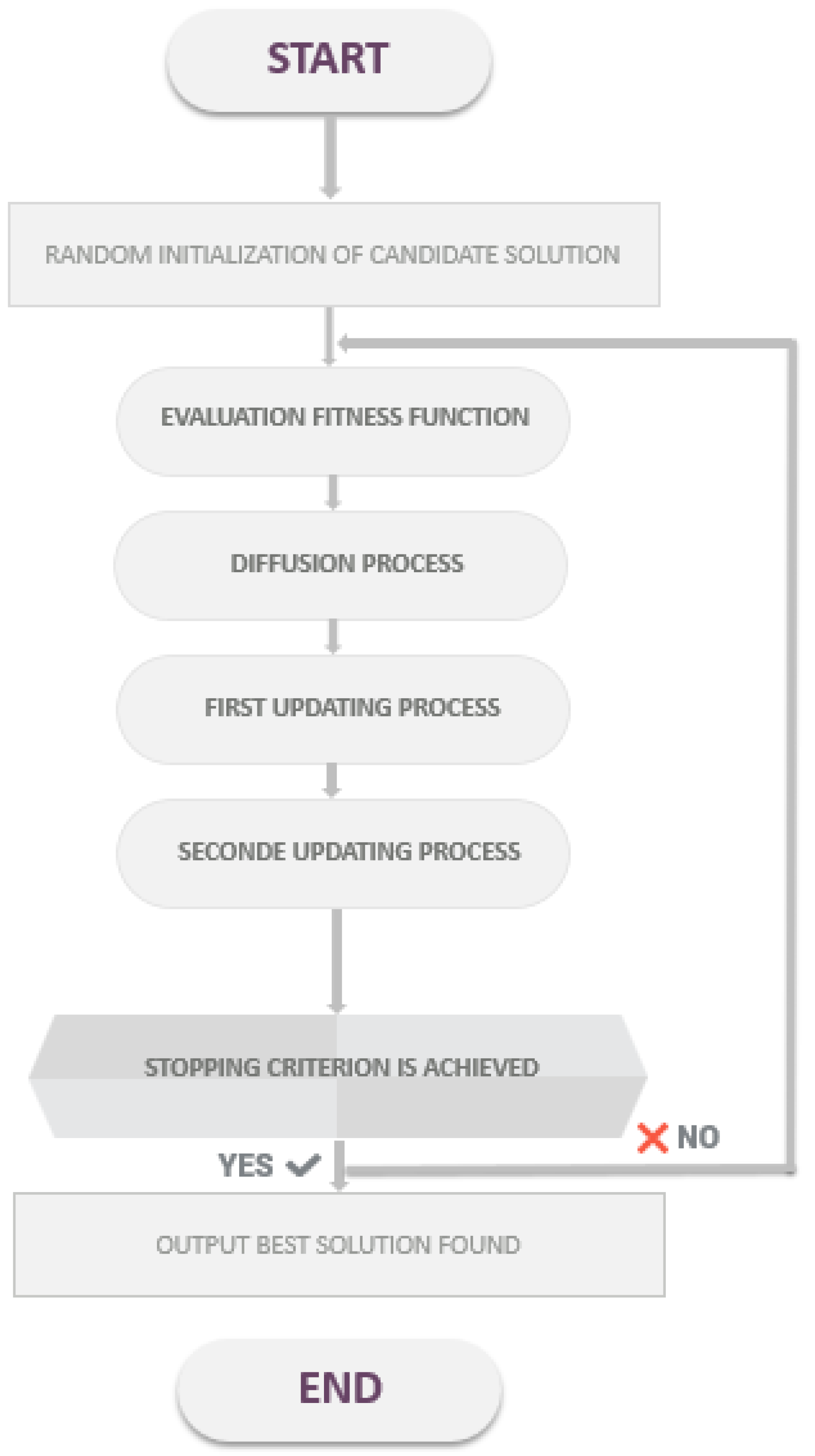
Algorithm 1 represents the SFS algorithm, where Figure 1 illustrates the SFS flowchart.

Algorithm 1 SFS algorithm

1: Initialize candidate solutions randomly 2: while Stopping Criterion is not achieved do 3:  Evaluate the candidate solutions using the fitness function 4:  Diffusion process (Equations (10) and (11)) 5:  1st updating process (Equation (12)) 6:  2nd updating process (Equations (13) and (14)) 7: end while

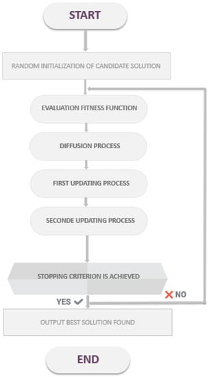
Figure 1. Flowchart of SFS algorithm.

3. Stability Analysis

3.1. Analysis with Quadratic Functions

In most cases, the results of stability analysis and stabilization for TSF systems, which are derived from LMI or BMI constraints, are obtained through the application of Lyapunov’s direct method.

In this subsection, we give a simple criterion to verify the stability of an autonomous TSF system using a QLF.

We have an autonomous TSF descriptor model

$${\displaystyle \dot{x}\left(t\right)=\sum _{i=1}^r{h}_i\left(x\right)A_{i}x}$$

(15)

Theorem 2

([4]). The TSF descriptor model (15) is said to be stable iff there exists $P=P^T>0$ such that the following matrix inequalities hold for each $i=1\dots n$

$$A_i^{T}P+P{A}_i+2\alpha P<0$$

(16)

(where $\alpha >0$) then the origin is globally asymptotically stable.

3.2. Analysis with Non-Quadratic Stability Functions

The next theorem shows the sufficient conditions that guarantee the asymptotic stability of an autonomous fuzzy system using LIFF.

Theorem 3.

For all $i,j=1,\dots ,r$, if there exist $\overline{H},E_i$, and $Q\ge 0$, which causes the linear matrix inequalities (17) and (19) to hold, the TSF descriptor model (15) is asymptotically stable

$$P_i=\overline{H}+E_i>0$$

(17)

$$\overline{H}{A}_i+A_i^T\overline{H}+E_i{A}_i+A_i^T{E}_i+(n-1)Q<0$$

(18)

$$\begin{array}{c}\overline{H}{A}_j+A_j^T\overline{H}+E_i{A}_j+A_j^T{E}_i+\overline{H}{A}_i+Y{A}_i^T\overline{H}\hfill \\ +E_j{A}_i+A_i^T{E}_j-2Q\le 0\hfill \end{array}$$

(19)

Proof. 

The time derivative of $V\left(x\right)$ is:

$${\displaystyle \dot{V}\left(t\right)=x^T\left\{\sum _{i=1}^r\sum _{j=1}^r{\mu }_i\left(t\right){\mu }_j\left(t\right)(P_i{A}_j+A_j^T{P}_i)\right\}x}$$

$$\begin{array}{c}{\displaystyle \dot{V}\left(t\right)=x^T\{\sum _{i=1}^r{\mu }_i^2\left(t\right)(P_i{A}_i+A_i^T{P}_i)+}\hfill \\ {\displaystyle \sum _{i=1}^r\sum _{j>i}^{}{\mu }_i\left(t\right){\mu }_j\left(t\right)(P_i{A}_j+A_j^T{P}_i+P_j{A}_i+A_i^T{P}_j)\}x}\hfill \end{array}$$

Based on the two last inequalities of (18) and (19) and the corollary (4) in [1]

$$\begin{array}{c}{\displaystyle \sum _{i=1}^r{\mu }_i^2\left(t\right)\ge \frac{1}{(s-1)}\sum _{j>i}^{r}2{\mu }_i\left(t\right){\mu }_j\left(t\right)}\hfill \end{array}$$

(20)

where $1<s\le r$ then,

$$\begin{array}{c}{\displaystyle \dot{V}\left(t\right)\le x^T\{2\sum _{i=1}^r\sum _{j>i}^r{\mu }_i\left(t\right){\mu }_j\left(t\right)Q}\hfill \\ {\displaystyle +\sum _{i=1}^r{\mu }_i^2\left(t\right)(P_i{A}_i+A_i^T{P}_i)\}x}\hfill \end{array}$$

$$\begin{array}{c}{\displaystyle \dot{V}\left(t\right)\le x^T\left\{\sum _{i=1}^r{\mu }_i^2\left(t\right)(A_i^T{P}_i+P_i{A}_i+(n-1)Q)\right\}x}\hfill \end{array}$$

$$\begin{array}{c}\dot{V}\left(t\right)<0\hfill \end{array}$$

□

4. Stabilization

The controller is designed using the classical state feedback.

$$u\left(t\right)=-F(x\left(t\right)-x_c\left(t\right))$$

(21)

where F is the controller gain to be designed, ($x\left(t\right),x_c\left(t\right)$) are the actual and desired states, respectively.

Throughout this paper, we assume that ($d{x}_c\left(t\right)/dt=0$), and then, the following theorem is used to derive the stability criteria.

Theorem 4.

For all $i,j=1,\dots ,r$, if there exist $\overline{H},E_i,{\mathcal{N}}_i$, and $Q\ge 0$, which make the linear matrix inequalities (27)–(29) hold, the TSF descriptor model (3) with the state feedback controller (21) is asymptotically stable

$${\mathcal{H}}_i=\overline{H}+E_i>0$$

(22)

$${\mathcal{H}}_i{\mathcal{A}}_i+{\mathcal{A}}_i^T{\mathcal{H}}_i-B_i{\mathcal{N}}_i-{\mathcal{N}}_i^T{B}_i^T+(n-1)Q<0$$

(23)

$$\begin{array}{c}{\mathcal{H}}_i{\mathcal{A}}_j+{\mathcal{A}}_j^T{\mathcal{H}}_i+{\mathcal{H}}_j{\mathcal{A}}_i+{\mathcal{A}}_i^T{\mathcal{H}}_j-B_j{\mathcal{N}}_i\hfill \\ -{\mathcal{N}}_i^T{B}_j^T-B_i{\mathcal{N}}_j-{\mathcal{N}}_j^T{B}_i^T-Q\le 0i<j\hfill \end{array}$$

(24)

where $\mathcal{N}=F{\mathcal{H}}_i$ and $\overline{H},E_i$ are defined by (22).

Proof. 

The closed loop of the TSF system (3) with the controller law (21) becomes:

$${\displaystyle \dot{x}\left(t\right)=\sum _{i=1}^r{\mu }_i\left(x\right)(A_i-B_{i}F)x\left(t\right)}$$

(25)

the dynamic of the state error with (21) can be represented as:

$$\dot{e}\left(t\right)=\dot{x}\left(t\right)-{\dot{x}}_c\left(t\right)$$

(26)

then

$$\begin{array}{c}\dot{e}\left(t\right)=(A_0-B_{0}F)e\left(t\right)+B_{0}F{x}_c\left(t\right)\hfill \\ +\{{\rm Y}\left(x\left(t\right)\right)-{\rm Y}\left(x_c\left(t\right)\right)\}\hfill \end{array}$$

(27)

where

$$\begin{array}{c}{\displaystyle A_0=1/r\sum _{i=1}^r{A}_i,B_0=1/r\sum _{i=1}^r{B}_i}\hfill \\ \overline{A_i}=A_i-A_0,\overline{B_i}=B_i-B_0\hfill \\ {\displaystyle {\rm Y}\left(x\left(t\right)\right)=\sum _{i=1}^r{\mu }_i\left(x\right)(\overline{A_i}x\left(t\right)-\overline{B_i}F)e\left(t\right)}\hfill \\ {\displaystyle {\rm Y}\left(x_c\left(t\right)\right)=\sum _{i=1}^r{\mu }_i\left(x\right)(\overline{A_i}-\overline{B_i}F)x_c\left(t\right)}\hfill \end{array}$$

The mean value theorem was exploited in order to define the nonlinear terms as:

$${\rm Y}\left(x\left(t\right)\right)-{\rm Y}\left(x_c\left(t\right)\right)={\displaystyle \frac{\partial {\rm Y}\left(x\right)}{\partial x}}\left(c\right)(x\left(t\right)-x_c\left(t\right))\mid {}_{x\left(t\right)<c<x_c\left(t\right)}$$

then,

$$\begin{array}{c}{\displaystyle \dot{e}\left(t\right)=\sum _{i=1}^{q=2^{n^2}}{\mu }_i\left(x\right)({\mathcal{A}}_i-B_{i}F)e\left(t\right)}\hfill \\ +\{B_{0}F{x}_c\left(t\right)+{\rm Y}\left(x_c\left(t\right)\right)\}\hfill \end{array}$$

(28)

where the matrices ${\mathcal{A}}_i$ are calculated with the relation (5).

Let $V\left(x\right)$ be a line-integral Lyapunov function, and its time derivative is

$$\begin{array}{c}\dot{V}\left(x\right)=x{\left(t\right)}^T\{{\mathcal{P}}_i{\mathcal{A}}_i+{\mathcal{A}}_i^T{\mathcal{P}}_i^T-{\mathcal{P}}_i{B}_{i}F\hfill \\ -F^T{B}_i^T{\mathcal{P}}_i\}x\left(t\right)\hfill \end{array}$$

(29)

let

$$\begin{array}{c}{\displaystyle \Pi \left(x\right)=\sum _{i=1}^r\sum _{j=1}^r{\mu }_i\left(x\right){\mu }_j\left(x\right)\{{\mathcal{P}}_i({\mathcal{A}}_j-B_{j}F)}\hfill \\ +({\mathcal{A}}_j^T-F^T{B}_j^T){\mathcal{P}}_i\}\hfill \end{array}$$

$${\displaystyle \begin{array}{c}{\displaystyle \Pi \left(x\right)=\sum _{i=1}^r{\mu }_i^2\left(x\right)\{{\mathcal{P}}_i({\mathcal{A}}_i-B_{i}F)+({\mathcal{A}}_i^T-F^T{B}_i^T){\mathcal{P}}_i\}}\\ +{\displaystyle \sum _{i=1}^r\sum _{j>i}}{\mu }_i\left(x\right){\mu }_j\left(x\right)\{{\mathcal{P}}_i({\mathcal{A}}_j-B_{j}F)+({\mathcal{A}}_j^T-F^T{B}_j^T){\mathcal{P}}_i\\ +{\mathcal{P}}_j({\mathcal{A}}_i-B_{i}F)+({\mathcal{A}}_i^T-F^T{B}_i^T){\mathcal{P}}_j\}\end{array}}$$

Utilizing the property (20), we can write:

$${\displaystyle \begin{array}{c}{\displaystyle \Pi \left(x\right)⩽2\sum _{i=1}^r\sum _{j>i}^{}{\mu }_i\left(x\right){\mu }_j\left(x\right)Q+}\hfill \\ {\displaystyle \sum _{i=1}^r}{\mu }_i^2\left(x\right)\{{\mathcal{P}}_i({\mathcal{A}}_i-B_{i}F)+({\mathcal{A}}_i^T-F^T{B}_i^T){\mathcal{P}}_i\}\end{array}}$$

$$\begin{array}{c}{\displaystyle ⩽\sum _{i=1}^r{\mu }_i^2\left(x\right)\{{\mathcal{P}}_i({\mathcal{A}}_i-B_{i}F)+({\mathcal{A}}_i^T-F^T{B}_i^T){\mathcal{P}}_i\}}\hfill \\ +(n-1)Q<0\end{array}$$

then, for all $x\ne 0$, $\dot{V}\left(x\right)=x{\left(t\right)}^T\Pi \left(x\right)x\left(t\right)<0$. □

5. Simulation Example

In this section, a numerical example is provided to show the effectiveness of the proposed relaxed stability and stabilization conditions.

Example

Consider the continuous TSF system given by the following rules:

$\hspace{1em}\hspace{1em}\hspace{1em}$IF$\hspace{1em}$${\chi }_1\left(t\right)$ is $M_{{}_{i}1}$

$$\mathbf{THEN} \dot{x}\left(t\right)=A_{i}x\left(t\right)+B_{i}u\left(t\right)$$

Using the nonlinear sector transformation, we can write:

$${\displaystyle \dot{x}\left(t\right)=\sum _{i=1}^2{h}_i\left(x\right)(A_{i}x\left(t\right)+B_{i}u\left(t\right))}$$

(30)

where

$$\begin{array}{c}{A}_1=\left[\begin{array}{c}-0.7-5a+2b\\ 1.4b+a-7\end{array}\right],B_1=B_2=\left[\begin{array}{c}0\\ 1\end{array}\right]\hfill \\ \\ A_2=\left[\begin{array}{c}0.1-5a+2b\\ -0.2b+a-7\end{array}\right]\hfill \end{array}$$

$$\begin{array}{c}{h}_1\left(t\right)={\displaystyle \frac{x_1\left(t\right)+1}{8}}\hfill \\ h_2\left(t\right)={\displaystyle \frac{7-x_2\left(t\right)}{8}};\hfill \end{array}$$

The pair ($a\in [-15,-5]$ and $b\in [-10,10]$) are adjusted to compare the feasible areas for Theorems 2 and 3.

In order to enhance control accuracy, the SFS method is used to find the appropriate $P_1,P_2$ and Q matrices.

Firstly, n candidate solutions are initialized randomly in the search space. Then, the diffusion and updating processes of SFS are applied for many iterations in order to find the best global solution that minimizes the following fitness function:

$$F={\alpha }_1\times F_1+{\alpha }_2\times F_2+{\alpha }_3\times F_3$$

with

$$\begin{array}{c}{F}_1=A_1^T\times P_1+P_1\times A_1+(n-1)\times Q\hfill \\ F_2=A_2^T\times P_2+P_2\times A_2+(n-1)\times Q\hfill \\ F_3=A_2^T\times P_1+P_1\times A_2+P_2\times A_1+A_1^T\times P_2-3\times Q\hfill \end{array}$$

Subject to:

$$P_1,P_2\mathrm{and}Q>0$$

The maximum number of solutions and iterations is fixed at 150.

The inequality (17)–(19) allows computing matrices $P_1,P_2,\mathrm{and}Q$

$$\begin{array}{c}{P}_1=\left[\begin{array}{c}0.03510.1276\\ 0.12760.7454\end{array}\right],P_2=\left[\begin{array}{c}0.14570.1161\\ 0.11610.6799\end{array}\right]\hfill \\ \\ Q=\left[\begin{array}{c}0.0710-0.0068\\ -0.00680.2172\end{array}\right]\hfill \end{array}$$

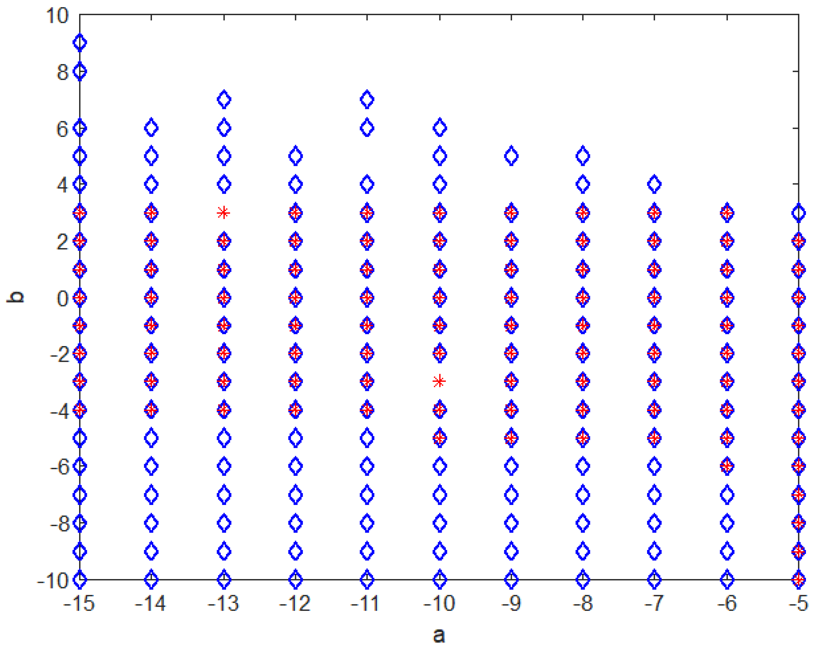
The feasible regions of the LMIs (25) using the SeDuMi solver and SFS algorithm can be shown in Figure 2. It is clear that there is a much bigger feasible region obtained with SFS than the SeDuMi Solver.

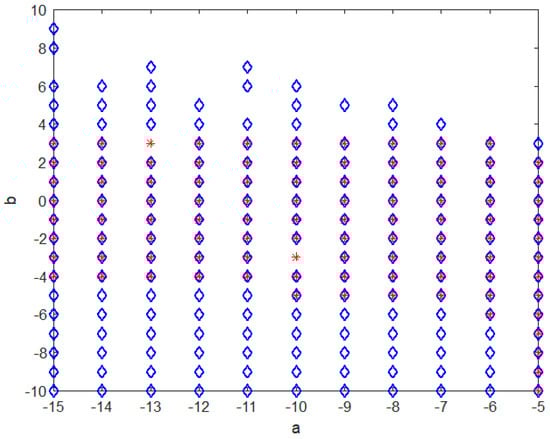
Figure 2. Feasibility fields obtained through Theorem 2 with the SeDuMi solver and SFS algorithm.

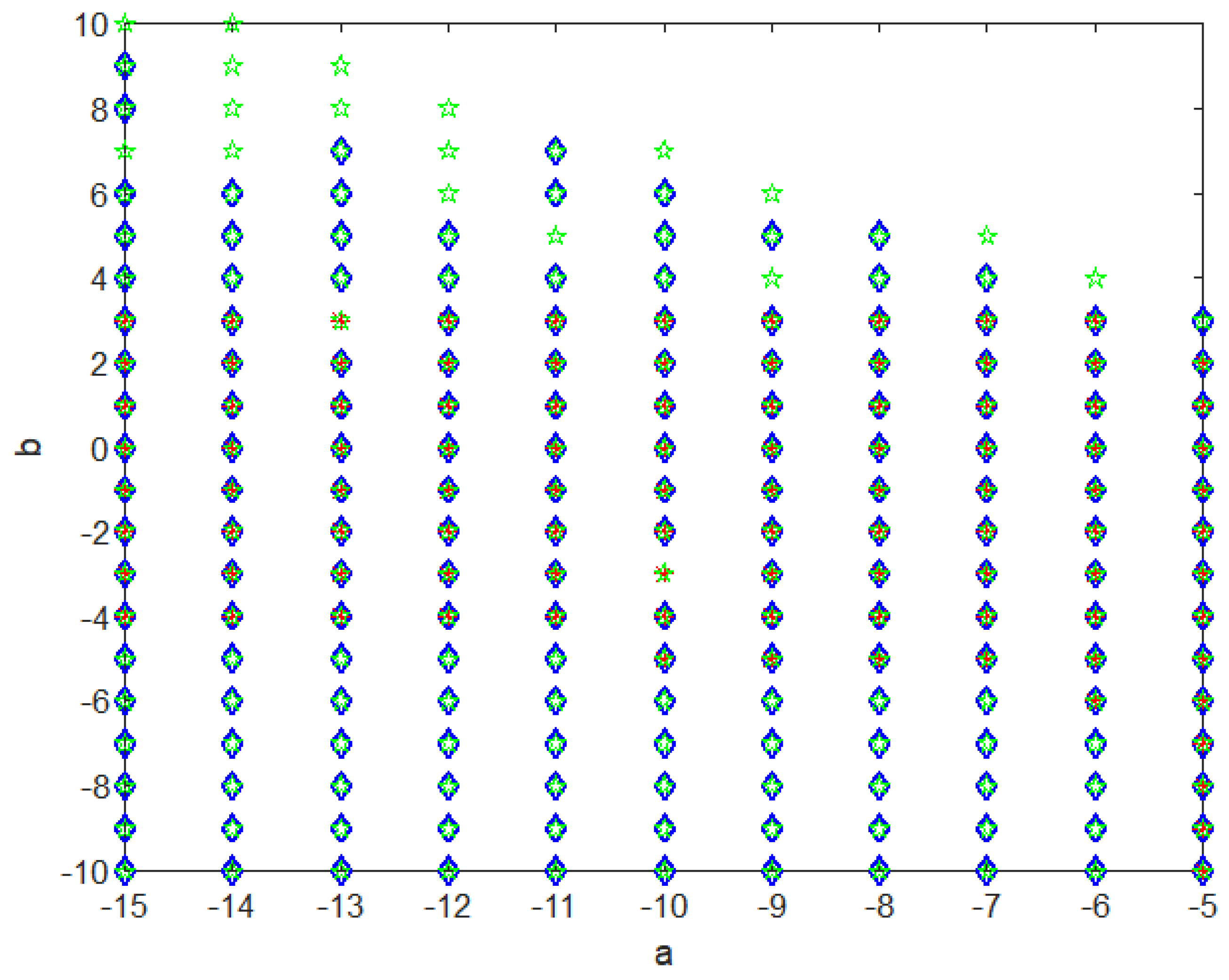
Figure 3 represents the stable region of the LMIs via Theorems 2 and 3. The feasible region obtained with Theorem 4 covers the stable region given by Theorem 3, which demonstrates that LMI constraints via non-quadratic functions are less conservative than the classical quadratic form.

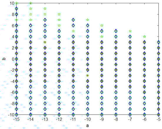
Figure 3. Comparison of the feasibility fields obtained through Theorems 2 and 3.

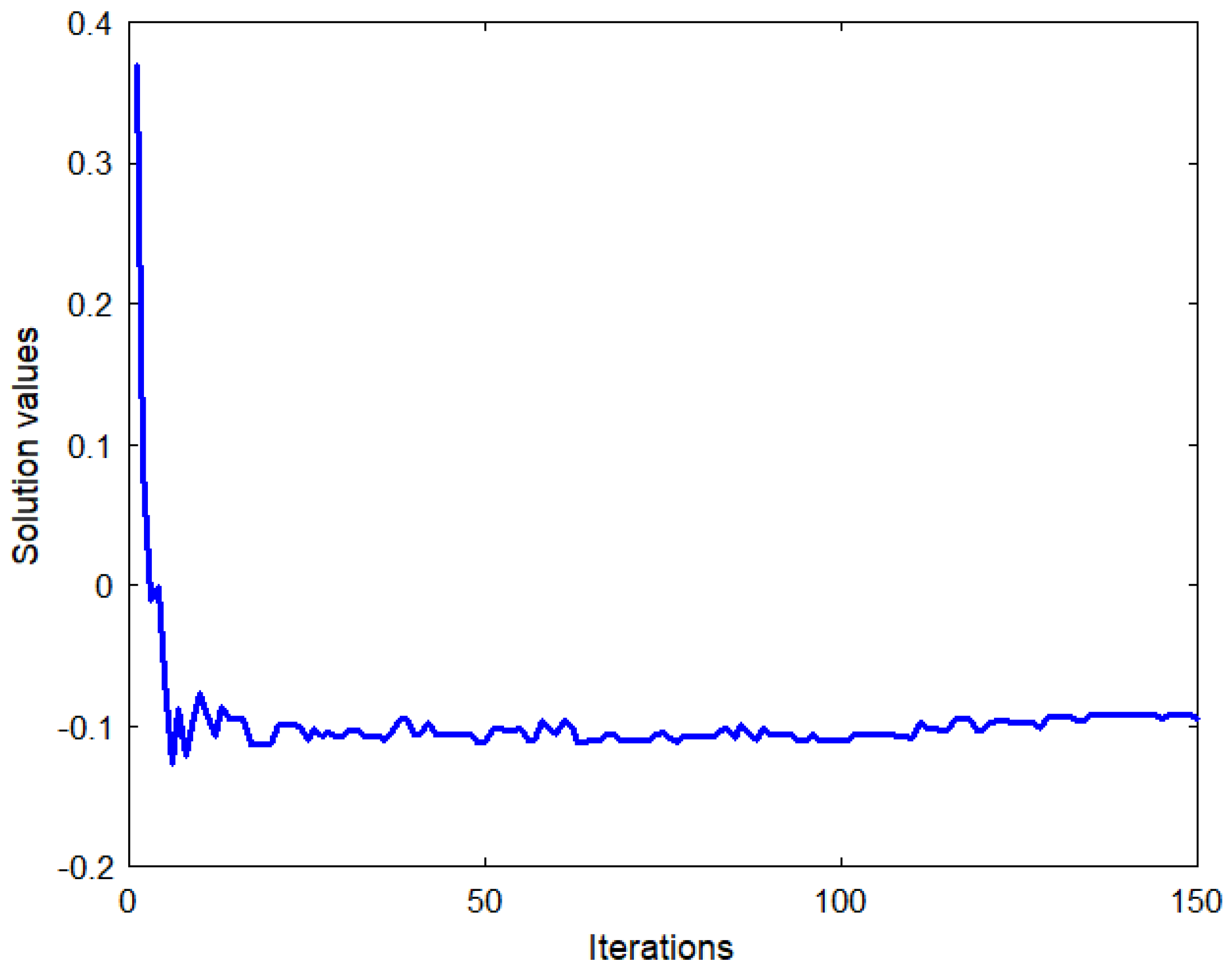
Figure 4 shows the trajectory of one candidate solution during the optimization process. The curve is an amortized sine wave when the solutions take far apart positions at the beginning to explore different regions, and then it concentrates the search in a small area.

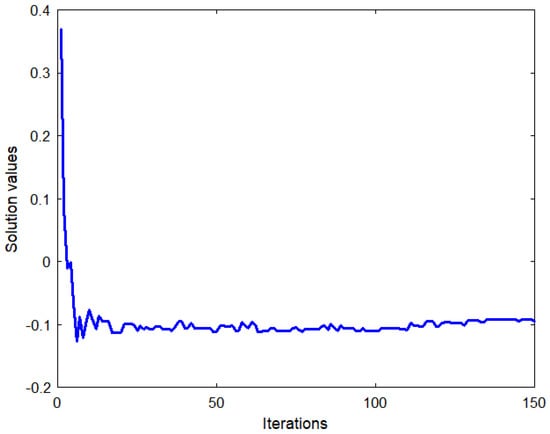
Figure 4. Trajectory of solution.

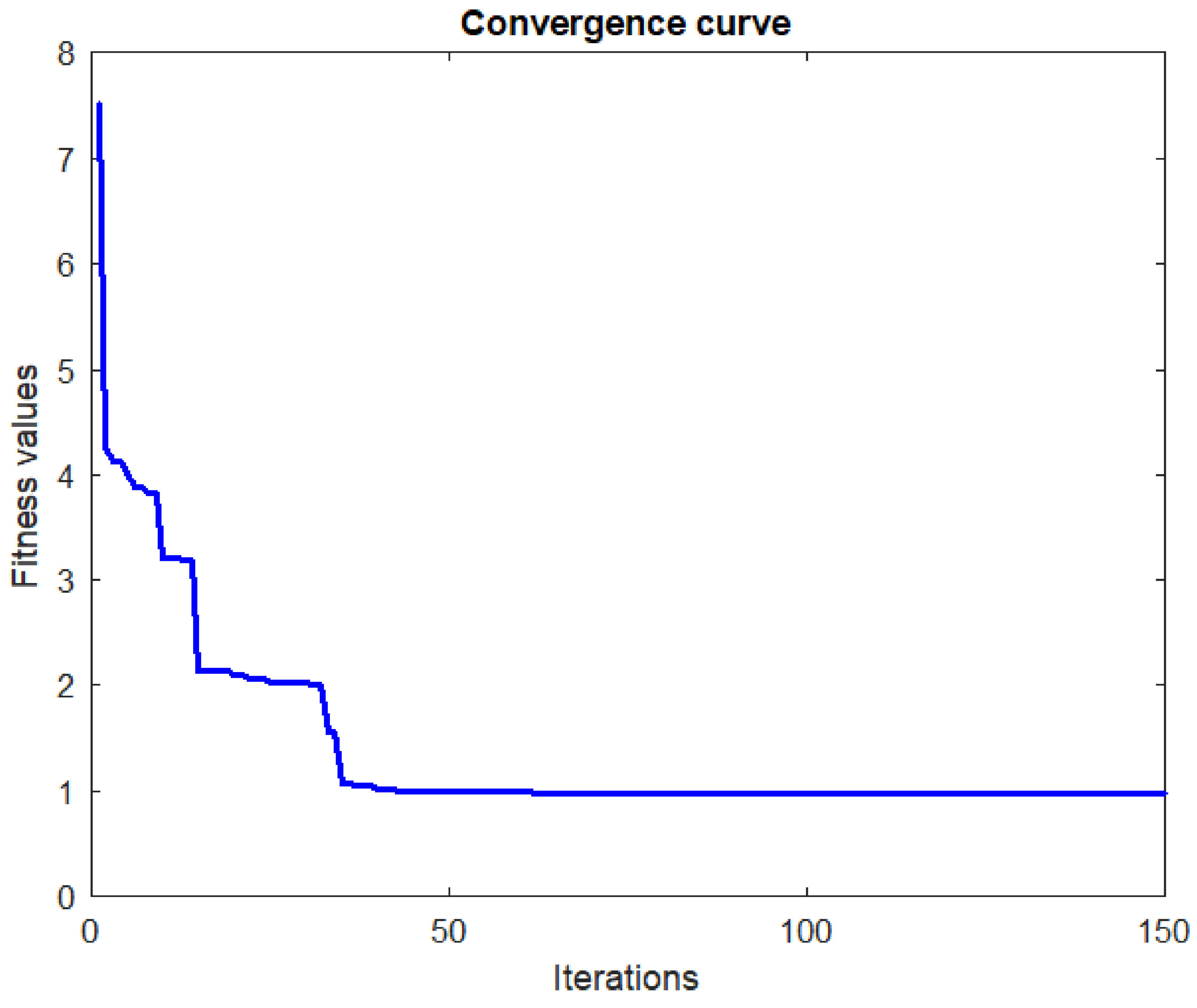
The convergence curve illustrated in Figure 5 shows the fitness values obtained during the iterations. It is clear that our fitness function was minimized successfully using the SFS method, and it needs only 50 iterations to reach a minimal fitness value, which proves the rapidity and robustness of our approach.

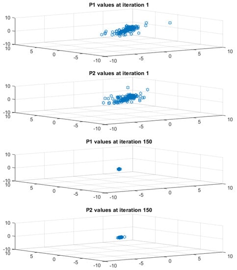
Figure 5. $P_i$ Values.

Remark 1.

Three runs of the algorithm were conducted, and then the standard deviation was calculated. The results show a small standard deviation of about 0.0189, which demonstrates that the proposed approach (SFS) is sufficiently robust.

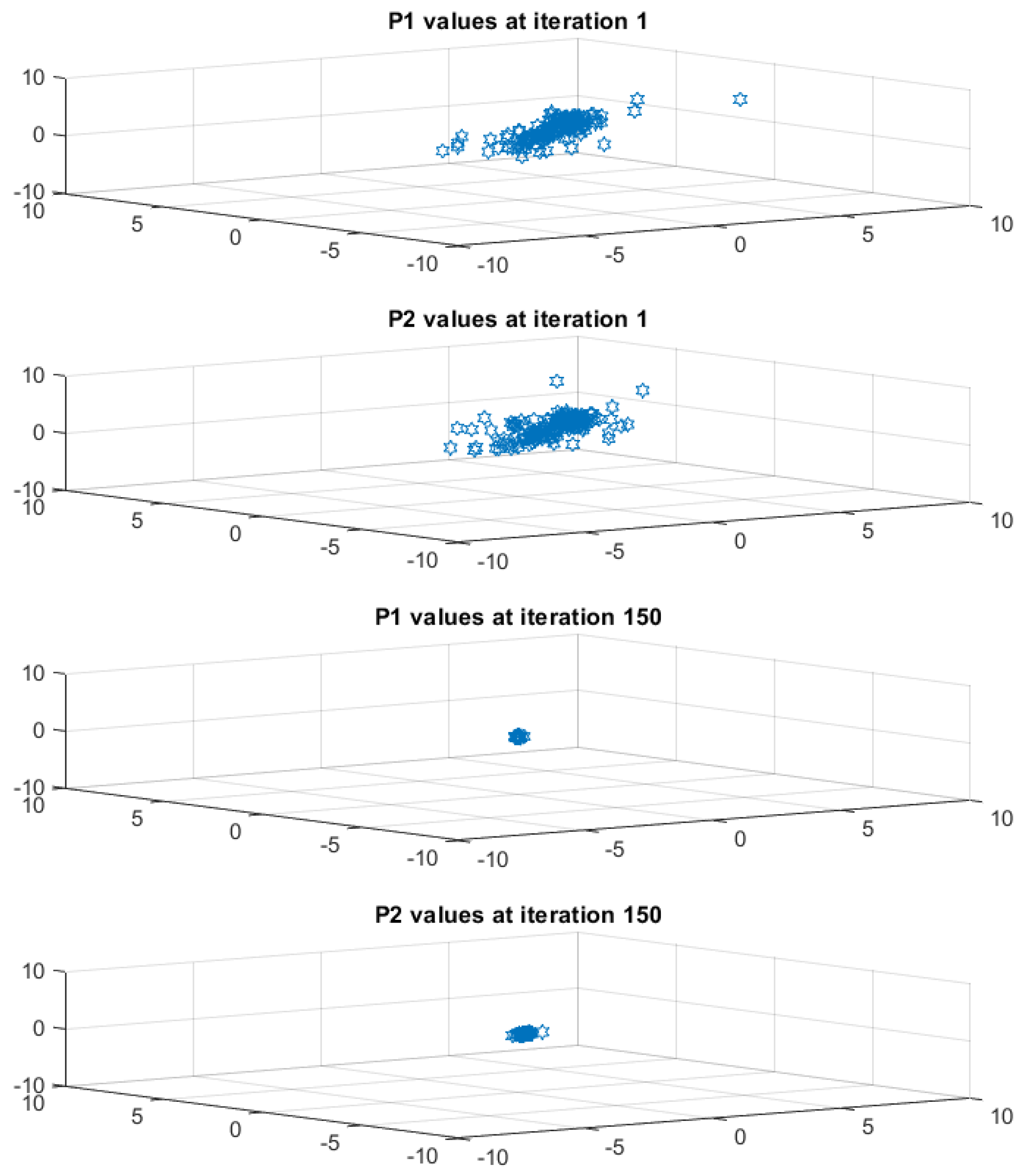
The movement of the candidate solutions are monitored in different iterations (iter = 1, iter = 75 and iter = 150). As can be seen from Figure 6, the solutions are first distributed in the search space in order to evaluate various possibilities, and then they begin to move and converge gradually to the global best solution.

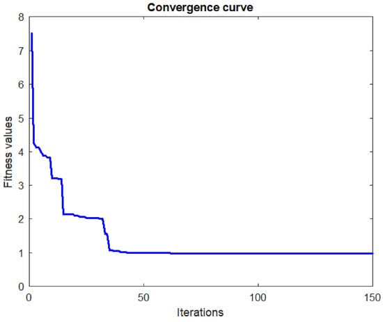
Figure 6. Fitness function.

When a = −14 and b = 10, the stabilization criteria through Theorem 2 are infeasible, meaning the stable controller cannot be obtained by these approaches. However, using Theorem 3, the stabilization conditions are solved under LMIs regions. The positive matrices are obtained as

$$\begin{array}{c}{P}_1=\left[\begin{array}{c}0.01100.0005\\ 0.00050.0109\end{array}\right],P_2=\left[\begin{array}{c}0.01100.0005\\ 0.00050.0118\end{array}\right]\hfill \\ \\ Q=\left[\begin{array}{c}0.23150.0384\\ 0.03840.2028\end{array}\right]\hfill \end{array}$$

and the controller gains

$$\begin{array}{c}F=\left[\begin{array}{c}0.4433-0.1695\end{array}\right]\hfill \end{array}$$

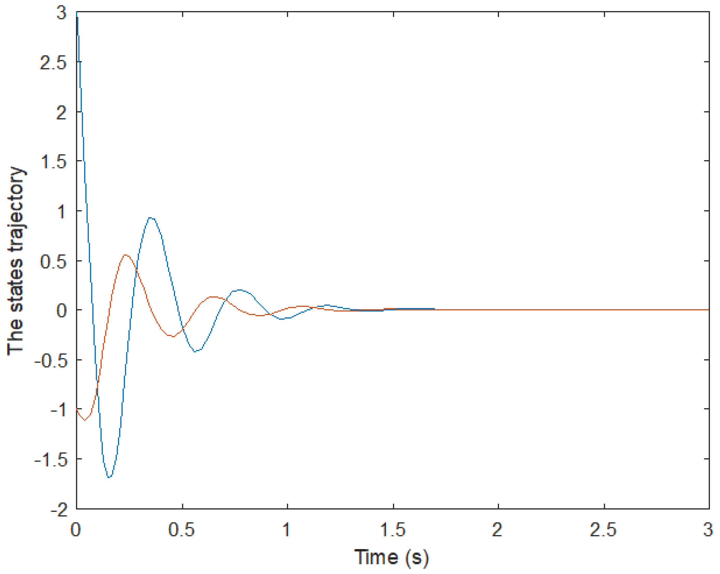
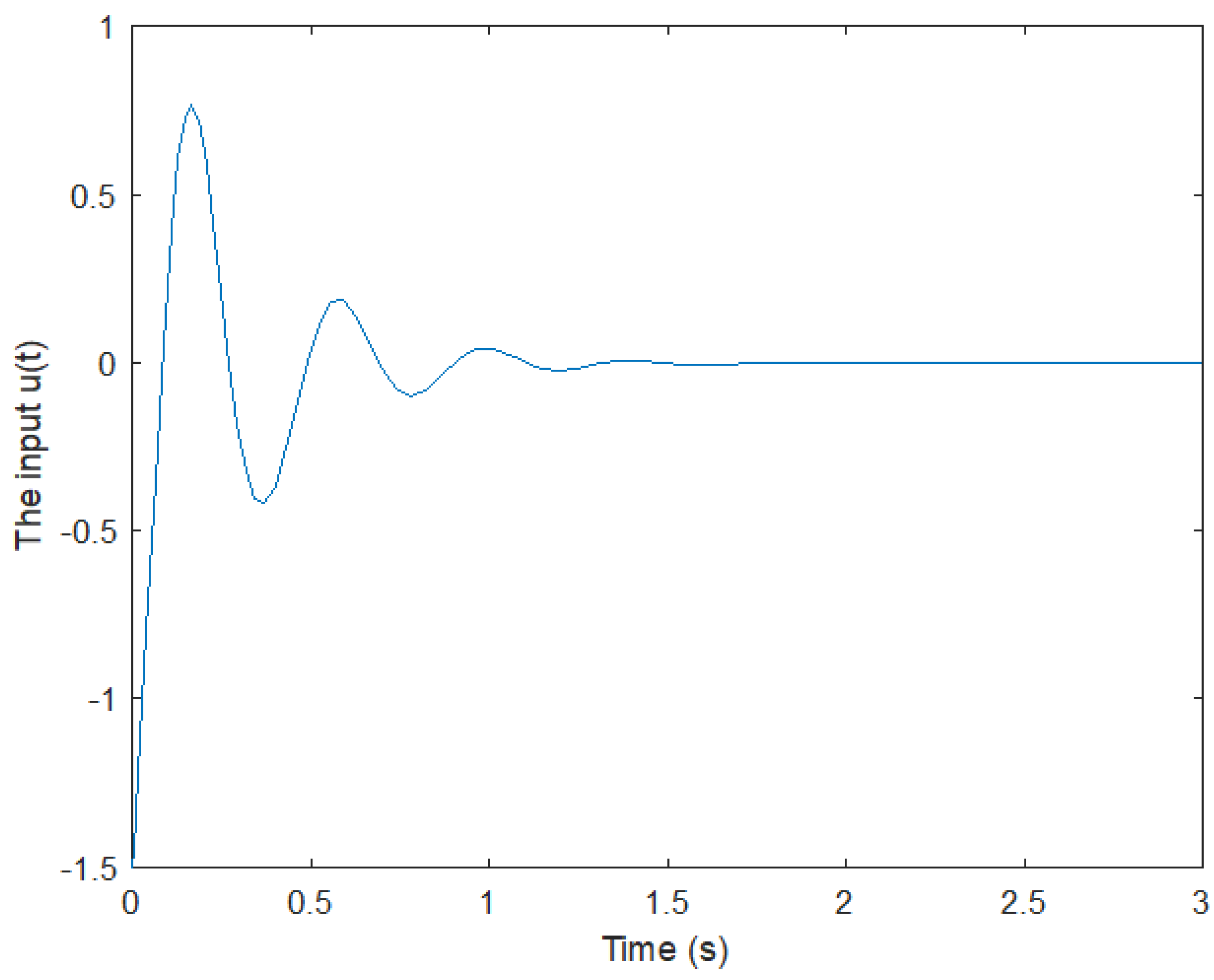
Figure 7 and Figure 8 represent the simulation results of the closed-loop state responses when the initial conditions are x(0) = [−3 1]. The state responses show that the proposed controller is stable. The control signal u(t) is shown in Figure 8.

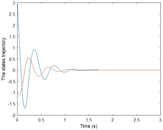
Figure 7. State trajectory.

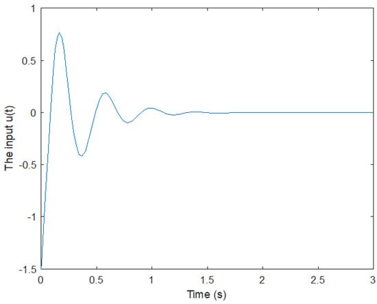
Figure 8. Input signal.

6. Conclusions and Future Works

The problem of stability and stabilization for TS fuzzy descriptor models has been investigated. Based on a non-quadratic Lyapunov function, novel sufficient conditions for stability and stabilization are obtained using a modified mean value theorem. Comparison results show that the derived stability conditions proved to cover more extensive feasibility regions than the quadratic Lyapunov function and exhibit less conservativeness. Moreover, the stabilization criteria are presented in terms of linear matrix inequalities instead of bilinear matrix inequalities conditions. A stochastic fractal search algorithm was used to solve the relaxed conditions. Finally, a numerical example was provided to prove the effectiveness of the proposed approach. In future work, based on the approach of the mean value theorem and the integral Lyapunov fuzzy function, we will establish a robust controller for a time-varying Takagi-Sugeno fuzzy system [24,25] and a fuzzy large-scale system [26].

References

- Tanaka, K.; Ikeda, T.; Wang, H.O. Fuzzy regulators and fuzzy observers: Relaxed stability conditions and LMI-based designs. IEEE Trans. Fuzzy Syst. 1998, 6, 250–265. [Google Scholar] [CrossRef]
- Zhang, J.; Wang, X.; Shao, X. Design and real-time implementation of Takagi-Sugeno fuzzy controller for magnetic levitation ball system. IEEE Access 2020, 8, 38221–38228. [Google Scholar] [CrossRef]
- Li, Z.; Wang, J.; Liu, H. A robust state estimator for TS fuzzy system. IEEE Access 2020, 8, 84063–84069. [Google Scholar] [CrossRef]
- Tanaka, K.; Wang, H.O. Fuzzy Control Systems Design and Analysis; John Wiley and Sons, Ltd.: Hoboken, NJ, USA, 2001. [Google Scholar]
- Chadli, M.; Karimi, H.R.; Shi, P. On stability and stabilization of singular uncertain Takagi-Sugeno fuzzy systems. J. Frankl. Inst. 2014, 351, 1453–1463. [Google Scholar] [CrossRef]
- Hammoudi, M.Y.; Allag, A.; Becherif, M.; Benbouzid, M.; Alloui, H. Observer design for induction motor: An approach based on the mean value theorem. Front. Energy 2014, 8, 426–433. [Google Scholar] [CrossRef]
- Pan, J.T.; Guerra, T.M.; Fei, S.M.; Jaadari, A. Nonquadratic stabilization of continuous T-S fuzzy models: LMI solution for a local approach. IEEE Trans. Fuzzy Syst. 2011, 20, 594–602. [Google Scholar] [CrossRef]
- Bouarar, T.; Guelton, K.; Manamanni, N. Robust fuzzy Lyapunov stabilization for uncertain and disturbed Takagi-Sugeno descriptors. Isa Trans. 2010, 49, 447–461. [Google Scholar] [CrossRef] [PubMed]
- Sala, A.; Arino, C. Relaxed stability and performance conditions for Takagi-Sugeno fuzzy systems with knowledge on membership function overlap. IEEE Trans. Syst. Man, Cybern. Part (Cybern.) 2007, 37, 727–732. [Google Scholar] [CrossRef] [PubMed]
- Peixoto, M.L.; Pessim, P.S.; Lacerda, M.J.; Palhares, R.M. Stability and stabilization for LPV systems based on Lyapunov functions with non-monotonic terms. J. Frankl. Inst. 2020, 357, 6595–6614. [Google Scholar] [CrossRef]
- Bernal, M.; Sala, A.; Lendek, Z. Stability Analysis. In Analysis and Synthesis of Nonlinear Control Systems; Elsevier: Amsterdam, The Netherlands, 2022; pp. 97–167. [Google Scholar]
- Wang, R.; Jiao, T.; Zhang, T.; Fei, S. Improved stability results for discrete-time switched systems: A multiple piecewise convex Lyapunov function approach. Appl. Math. Comput. 2019, 353, 54–65. [Google Scholar] [CrossRef]
- Della Rossa, M.; Goebel, R.; Tanwani, A.; Zaccarian, L. Piecewise structure of Lyapunov functions and densely checked decrease conditions for hybrid systems. Math. Control Signals Syst. 2021, 33, 123–149. [Google Scholar] [CrossRef]
- Lazarini, A.Z.; Teixeira, M.C.; Jean, M.D.S.; Assunção, E.; Cardim, R.; Buzetti, A.S. Relaxed Stabilization Conditions for TS Fuzzy Systems With Optimal Upper Bounds for the Time Derivative of Fuzzy Lyapunov Functions. IEEE Access 2021, 9, 64945–64957. [Google Scholar] [CrossRef]
- Fan, X.; Wang, Z. A Fuzzy Lyapunov Function Method to Stability Analysis of Fractional Order TS Fuzzy Systems. IEEE Trans. Fuzzy Syst. 2021, 30, 2769–2776. [Google Scholar]
- Ku, C.C.; Yeh, Y.C.; Lin, Y.H.; Hsieh, Y.Y. Fuzzy static output control of T-S fuzzy stochastic systems via line integral Lyapunov function. Processes 2021, 9, 697. [Google Scholar] [CrossRef]
- Okwu, M.O.; Tartibu, L.K. Metaheuristic Optimization: Nature-Inspired Algorithms Swarm and Computational Intelligence, Theory and Applications; Springer: Berlin/Heidelberg, Germany, 2020. [Google Scholar]
- Salimi, H. Stochastic fractal search: A powerful metaheuristic algorithm. Knowl.-Based Syst. 2015, 75, 1–18. [Google Scholar] [CrossRef]
- Rhee, B.J.; Won, S. A new fuzzy Lyapunov function approach for a Takagi-Sugeno fuzzy control system design. Fuzzy Sets Syst. 2006, 157, 1211–1228. [Google Scholar] [CrossRef]
- Hammoudi, M.Y.; Benbouzid, M.H.; Rizoug, N. New state observer based on Takagi-Sugeno fuzzy controller of induction motor. In Proceedings of the 4th International Conference on Systems and Control (ICSC), Sousse, Tunisia, 28–30 April 2015; IEEE: Piscataway, NJ, USA, 2015; pp. 145–150. [Google Scholar]
- Wang, H.O.; Tanaka, K. Fuzzy Control Systems Design and Analysis: A Linear Matrix Inequality Approach; John Wiley and Sons: Hoboken, NJ, USA, 2004. [Google Scholar]
- Phanomchoeng, G.; Rajamani, R.; Piyabongkarn, D. Nonlinear observer for bounded Jacobian systems, with applications to automotive slip angle estimation. IEEE Trans. Autom. Control 2011, 56, 1163–1170. [Google Scholar] [CrossRef]
- Betka, A.; Terki, N.; Toumi, A.; Hamiane, M.; Ourchani, A. A new block matching algorithm based on stochastic fractal search. Appl. Intell. 2019, 49, 1146–1160. [Google Scholar] [CrossRef]
- Cai, X.; Zhong, S.; Wang, J.; Shi, K. Robust H∞ control for uncertain delayed TS fuzzy systems with stochastic packet dropouts. Appl. Math. Comput. 2020, 385, 125432. [Google Scholar]
- Kau, S.W.; Lee, H.J.; Yang, C.M.; Lee, C.H.; Hong, L.; Fang, C.H. Robust H∞ fuzzy static output feedback control of TS fuzzy systems with parametric uncertainties. Fuzzy Sets Syst. 2007, 158, 135–146. [Google Scholar] [CrossRef]
- Hosseinzadeh, M.; Sadati, N.; Zamani, I. H∞ disturbance attenuation of fuzzy large-scale systems. In Proceedings of the IEEE International Conference on Fuzzy Systems (FUZZ-IEEE 2011), Taipei, Taiwan, 27–30 June 2011; IEEE: Pisacatway, NJ, USA, 2011; pp. 2364–2368. [Google Scholar]
Publisher’s Note: MDPI stays neutral with regard to jurisdictional claims in published maps and institutional affiliations. |
© 2022 by the authors. Licensee MDPI, Basel, Switzerland. This article is an open access article distributed under the terms and conditions of the Creative Commons Attribution (CC BY) license (https://creativecommons.org/licenses/by/4.0/).