Deep Clustering by Graph Attention Contrastive Learning

Abstract

Contrastive learning shows great potential in deep clustering. It uses constructed pairs to discover the feature distribution that is required for the clustering task. In addition to conventional augmented pairs, recent methods have introduced more methods of creating highly confident pairs, such as nearest neighbors, to provide more semantic prior knowledge. However, existing works only use partial pairwise similarities to construct semantic pairs locally without capturing the entire sample’s relationships from a global perspective. In this paper, we propose a novel clustering framework called graph attention contrastive learning (GACL) to aggregate more semantic information. To this end, GACL is designed to simultaneously perform instance-level and graph-level contrast. Specifically, with its novel graph attention mechanism, our model explores more undiscovered pairs and selectively focuses on informative pairs. To ensure local and global clustering consistency, we jointly use the designed graph-level and instance-level contrastive losses. Experiments on six challenging image benchmarks demonstrate the superiority of our proposed approach over state-of-the-art methods.

1. Introduction

Recently, research on unsupervised learning has become increasingly important due to the high cost of labeling large-scale datasets in supervised learning. As an important branch of unsupervised learning, clustering can group similar samples according to their underlying distribution without any labels; as a result, it has become increasingly crucial in many applications, such as facial expression recognition [1], video action recognition [2], recommendation systems [3], and domain adaptation [4,5,6] due to its good hidden correlation exploiting capability.

Conventional clustering methods, such as KMeans [7], spectral clustering [8], and subspace clustering, have been widely utilized, but they cannot perform satisfactorily when dealing with excessively high-dimensional data. To tackle this issue, deep clustering [9,10,11,12] methods use deep neural networks to achieve better representations. Owing to the powerful modelling capacities of deep learning networks, deep clustering methods have achieved fairly remarkable results.

As a representative branch of self-supervised learning, contrastive learning (CL) [13,14] jointly uses various augmentations and contrastive losses to learn discriminative representations. It shows great potential in real-world clustering scenarios [15,16] since it can make up for a lack of labels by naturally constructing augmented pairs. Inspired by the introduction of informative pairs, subsequent methods [17,18,19] have proposed to construct semantically confident pairs to guide the training process. SCAN [19] regards samples and their nearest neighbors as the most semantic pairs. NNM [18] extends the matching process for the nearest neighbors from a mini-batch to the overall feature.

Although their approaches can provide more semantic prior knowledge to the model, the exploration of semantic relations is restricted to the mining of local information. As shown in Figure 1, traditional CL only selects semantic pairs with the highest confidence scores or the smallest distance. Since the number of cluster partitions is much smaller than that of samples, the samples and their second-nearest neighbors are likely to belong to the same cluster; however, they are excluded in traditional CL, resulting in abundant false-negative pairs. Furthermore, traditional CL only requires pairwise constraints on samples and does not guarantee the consistency of overall sample distributions.

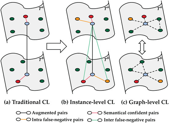
Figure 1. (a) Traditional contrastive learning with limited sample pair constraints. (b,c) Our proposed instance-level and graph-level contrastive learning, with more exploration on semantic sample pairs and more constraints on the overall sample distribution.

To address the problems above, we propose a novel deep graph attention contrastive learning framework (GACL). It simultaneously utilizes instance-level and graph-level contrasts to explore latent semantic relationships. Specifically, to contain more possible semantic pairs, e.g., false-negative pairs, GACL is performed across the K-nearest neighbor graph. Additionally, a novel graph attention mechanism is designed to selectively focus on the most informative pairs and eliminate deviated neighbors. The attention mechanism reweights the distance score based not only on the distance but also on the relative position of the samples in the graph.

Furthermore, we introduce instance-level and graph-level contrastive losses to ensure local and global clustering consistency. The instance-level loss supplements the false-negative sample constraints that were ignored in the previous methods, including the comparisons of inter-graph and intra-graph pairs (orange and green lines in Figure 1). Compared with the instance-level pairwise constraints, the graph-level loss has a constraint on the overall distributions of samples under two different augmentation, i.e., constraints on relationships between samples and their neighbors. Experimental results on six challenging datasets validate the effectiveness of the proposed method. We also perform an extensive ablation analysis to demonstrate the superiority of GACL.

The contributions of this paper can be summarized as follows:

• We propose a novel graph attention contrastive learning framework. By selecting and filtering samples through our graph attention framework, we can introduce more confident and informative semantic pairs to the clustering task and thus further improve clustering performance.
• Instance-level contrastive learning treats the local false-negative pairs as positive pairs, including the inter-graph and intra-graph situations. Meanwhile, the graph-level contrastive learning constrains neighbors’ relationships from a global perspective.
• We conduct extensive experiments on the image clustering task, and our proposed method achieves significant improvements on various datasets. We also conduct extensive ablation and case studies to validate the effectiveness of each proposed module.

2. Related Work

Our method aims to solve the problem of deep clustering using contrastive learning. In this section, we briefly overview some developments of deep clustering and contrastive learning.

2.1. Deep Clustering

Benefiting from the powerful representation ability of deep neural networks, deep clustering [9,10] has shown promising performance on complex datasets. Various methods have been proposed to combine feature learning and clustering and have achieved great success. For example, JULE [11] combines the hierarchical agglomerative clustering idea with deep learning with a recurrent framework that merges the clusters that are close to each other. Analogously, DeepClustering [12] groups the features using k-means and updates the deep network according to the cluster assignments in turn. However, their performances are likely to be unstable due to the accumulation of errors during alternation. Simultaneously, some online clustering methods have been proposed to jointly learn representations and cluster assignments. For example, IIC [16] discovers clusters by maximizing mutual information between the cluster assignments of data pairs. DCN [20] adopts auto-encoder and K-means to estimate cluster assignment and learn a “clustering-friendly” latent space. These approaches achieve good results, but they ignore the connections between cluster assignment learning and representation learning. As a contrast, our method considers their connections and simultaneously learns both feature representation and cluster assignment.

2.2. Graph-Based Clustering

Graph-based clustering is a fundamental yet challenging task that aims to reveal the underlying graph-based relationship structure and divides the nodes into several disjoint groups. The existing deep graph clustering methods can be roughly categorized into three classes according to their learning mechanisms: generative methods [21,22,23,24], adversarial methods [25,26,27], and contrastive methods [28,29,30]. The pioneer graph clustering algorithm MGAE [31] embeds nodes into the latent space with GAE [32] and then performs clustering over the learned node embeddings. Subsequently, DAEGC and MAGCN [33] improved the clustering performance of earlier works with the use of attention mechanisms [34]. GALA [35] and AGC [36] enhanced the performance of GAE with the use of a symmetric decoder and high-order graph convolution operation, respectively. In addition, ARGA [25] and AGAE [27] improved upon the discriminative capability of samples through adversarial mechanisms. Moreover, SDCN [22], AGCN [24], and DFCN [23] verify the effectiveness of the attribute–structure fusion mechanisms to improve the clustering performance. Although they have been verified to be effective, since most of these methods adopt a clustering-guided loss function to force the learned node embeddings to have the minimum amount of distortion against the pre-learned clustering centers, their clustering performance is highly dependent on good initial cluster centers, thus leading to manual trial-and-error pre-training. As a consequence, their performance consistency, as well as their convenience of implementation, is largely decreased. Unlike the above methods, however, our proposed method replaces the clustering-guided loss function by designing a novel neighbor-oriented contrastive loss function, thus eliminating the need for trial-and-error-based pretraining.

2.3. Deep Contrastive Clustering

Contrastive learning is an attention-getting unsupervised representation learning method with the goal of maximizing the similarities of positive pairs while minimizing those of negative pairs in a feature space. This learning paradigm has lately achieved promising performance in computer vision. Recently, contrastive learning [37], which utilizes self-supervisory information to discriminate each instance, has shown great potential in deep clustering. The basic idea of contrastive learning is to map the original data to a feature space wherein the similarities of positive pairs are maximized, while those of negative pairs are minimized. Contrastive clustering could be constructed using the following two strategies under an unsupervised setting. One is to use clustering results as pseudo-labels to guide the construction of pairs [38]. The other, which is more direct and commonly used, is to construct data pairs through data augmentation [39] and guiding the training. To be specific, the positive pair is composed of two augmented views of the same instance, and the other pairs are defined as negative pairs. For example, DAC [40] adopts a binary pairwise classification framework for image clustering to make the feature learning occur in a “supervised” manner. CC [15] treats cluster labels as special representations so that instance- and cluster-level representation learning can be conducted in the row and column spaces, respectively. The latest works are mostly based on mining semantic information outside the augmented pair. DCCM [17] comprehensively explores the correlation between negative and positive pairs with triplet mutual information loss [41]. PICA [42] introduced a partition uncertainty index to quantify the global confidence of the clustering assignment. SCAN [19] provides more semantic prior knowledge by mining nearest neighbors. NNM [18] further improves clustering performance by matching the nearest neighbor from both the batch and overall features.

Despite achieving remarkable improvements, existing works are still restricted to the mining of local information. Many informative semantic pairs are regarded as negative pairs, yielding semantically less plausible results. Our method addresses this limitation by extending pairwise semantic relationships to graph-wise ones. This technique helps us discover various high-confidence relationships behind the data and simultaneously allows the learning of cluster-friendly representations and compact cluster assignments from a global perspective.

3. Method

In the following section, the notation, definition, and the basic concept of contrastive learning are first introduced, followed by detailed descriptions of each module of our method. GACL can be adaptively integrated to any contrastive learning framework to provide more semantic relationships with its plug-and-play property.

3.1. Preliminaries

Given a set of unlabeled images $I=\{I_1,I_2,\cdots ,I_N\}$, deep clustering aims to learn (1) a feature embedding network that maps images into a compact vector subspace containing key semantic information; i.e., $f_{\theta }:I\to x\in {\mathbb{R}}^d$, where d is the embedding dimension; and (2) a classifier, $\varphi$, that projects the feature vectors into C partitions, i.e., $f_{\varphi }:x\to y,$$y\in \{1,2,\cdots ,C\}$, expecting that similar samples are grouped into the same cluster, while dissimilar ones are divided into different clusters.

Due to its powerful representation ability, contrastive learning is used to obtain discriminative representations, which learn the intrinsic data structure without any additional supervisory signals. Specifically, given an image instance $I_i$, it is applied with two random data transformations $T_a$ and $T_b$ from the same family of augmentations $\mathbb{T}$, resulting in two samples denoted as $t_{ai}=T_a\left(I_i\right)$ and $t_{bi}=T_b\left(I_i\right)$. The previous works have suggested that a proper choice of augmentation strategy is essential to achieving a good performance in downstream tasks. In this work, five types of data augmentation methods are used (see Section 4.3 for more details). Then, one shared deep neural network $f_{\theta }(·)$ is used to extract features for the augmented samples via $x_{ai}=f_{\theta }\left(t_{ai}\right)$ and $x_{bi}=f_{\theta }\left(t_{bi}\right)$. As for the architecture of the network, theoretically, our method does not depend on a specific network. Here, we simply adopt ResNet-18 as the backbone for a fair comparison.

Contrastive learning regards different augmented versions of an image as positive pairs, while different images in a mini-batch are taken as negative pairs. The loss functions are designed to pull positive pairs together and push negative ones away. The most common contrastive loss is InfoNCE, which is defined as follows:

$$\begin{array}{c}\hfill {\mathcal{L}}_{\mathrm{NCE}}(x_{ai},x_{bi})=-log\frac{\psi (x_{ai},x_{bi})}{\psi (x_{ai},x_{bi})+{\sum }_{j=1}^B{\mathbf{1}}_{j\ne i}\psi (x_{ai},x_{bj})}\\ \hfill -log\frac{\psi (x_{bi},x_{ai})}{\psi (x_{bi},x_{ai})+{\sum }_{j=1}^B{\mathbf{1}}_{j\ne i}\psi (x_{bi},x_{aj})},\end{array}$$

(1)

$$\psi (x_{ai},x_{bj})=exp(sim(x_{ai},x_{bj})/\tau ),$$

(2)

where $\tau$ is the temperature parameter, B is the batch size, and $sim(·)$ represents the cosine similarity between two input vectors. ${\mathbf{1}}_{j\ne i}$ is an indication function; when $j\ne i$, its value is 1, but otherwise, its value is 0. Obviously, in Equation (1), for a sample $x_{pi},p\in \{a,b\}$, this classic loss includes constraints on its one positive pair and $2B-2$ negative pairs.

3.2. Framework

As shown in Figure 2, our framework consists of three jointly learned components, namely, a graph construction layer that builds a nearest neighbor graph based on latent representations, a graph attention layer to selectively focus on informative pairs, and a pair of instance-level and graph-level contrastive losses for local and global constraints on the cluster assignments. We present the details of GACL below.

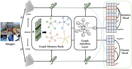
Figure 2. The overall structure of GACL. It consists of three jointly learned components, namely, a graph construction layer that builds a nearest neighbor graph based on the latent representation, a graph attention layer to selectively focus on informative pairs, and a pair of instance-level and graph-level contrastive losses for local and global constraints on the cluster assignments.

3.2.1. Graph Construction Layer

In a mini-batch, we assume that the representations generated by the backbone form a set, denoted as $X\in {\mathbb{R}}^{2B\times d}$, where d is the dimension of the embedding features. However, the deep learning model usually fluctuates during training, resulting in representation bias after each epoch. We take advantage of the moving average to obtain robust representations before the construction of the graph. To be specific, assuming that $x_{pi}^{\left(t\right)},p\in \{a,b\}$ is generated in the t-th epoch, the moving average of the representation can be defined as

$${\overline{x}}_{pi}^{\left(t\right)}=\frac{\alpha x_{pi}^{\left(t\right)}+(1-\alpha )x_{pi}^{(t-1)}}{\left|\right|\alpha x_{pi}^{\left(t\right)}+(1-\alpha )x_{pi}^{(t-1)}{\left|\right|}_2},i=1,2,\cdots ,B,$$

(3)

where $\alpha$ is a parameter for the trade-off of current and past effects and ${\overline{v}}_{pi}^{\left(0\right)}=v_{pi}^{\left(0\right)}$.

As demonstrated in [18], nearest neighbors provide important supervision information, which could be viewed as positive samples of the original samples. However, the nearest mining method only captures partial semantic relationships. To discover more available potential relationships, we propose to construct the entire K-nearest neighbor (KNN) graph instead of only using the nearest neighbor pairs. The KNN graph is constructed as follows:

$$\begin{array}{c}\hfill A_{p,i,j}^{\left(t\right)}=\left\{\begin{array}{cc}1,\hfill & \mathrm{if}{\overline{x}}_{pj}^{\left(t\right)}\in {\mathcal{N}}^k\left({\overline{x}}_{pi}^{\left(t\right)}\right)\mathrm{or}{\overline{x}}_{pi}^{\left(t\right)}\in {\mathcal{N}}^k\left({\overline{x}}_{pj}^{\left(t\right)}\right)\hfill \\ 0,\hfill & \mathrm{otherwise}\hfill \end{array}\right.,\end{array}$$

(4)

where ${\mathcal{N}}^k$ is the K-nearest neighbors and $i,j\in \{1,\dots ,B\}$.

3.2.2. Graph Attention Layer

The construction of the KNN graph helps us consider more confidence sample pairs. However, while alleviating the problem of false-negative samples, this method also introduces redundant noise, resulting in semantic pairs with low confidence being included. Therefore, how to select the appropriate semantic pair is still a very critical issue.

As we mentioned before, even if relatively closer samples can be found through KNN, it is not reasonable to simply classify them into the same category as the target sample. There exist two common situations: (1) it is not simple to choose a suitable value of k so that the number of selected neighbors is not higher or lower, as shown in Figure 3a; (2) if two samples with close distances are on the classification boundary, their other neighbors might belong to different classes, as shown in Figure 3b. In these situations, it is biased to judge the semantic relationships based only on the pairwise distance.

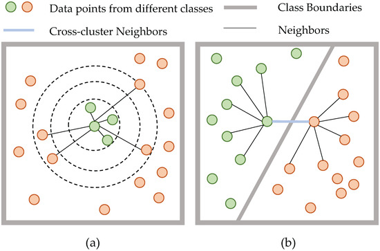
Figure 3. Two situations in which samples with close distances might not belong to one cluster. (a) Hard to set a suitable number of the neighbors, (b) two samples with close distances may have different neighbors set.

In order to solve the above problems, we designed a graph attention mechanism to comprehensively consider pairwise similarities and all relationships between samples in the latent space. The attention mechanism is normalized via softmax as follows:

$${\alpha }_{pij}=\frac{exp\left(score(x_{pi},x_{pj})\right)}{{\sum }_{t\in {\mathcal{N}}^k\left(pi\right)}exp\left(score(x_{pi},x_{pt})\right)},$$

(5)

where $score(·)$ is an alignment function that measures the relationship between the target sample and its neighbor. $score(·)$ can be any measured function such as cosine similarity. Here, $score(·)$ is defined as the output of the following feed-forward network with a single hidden layer:

$$score(x_{pi},x_{pj})=\sigma ({\mathbf{W}}^T[x_{pi}\left|\right|x_{pj}]+\mathbf{b}),$$

(6)

where $\sigma$ is a non-linear transformation, $\mathbf{W}$ is the weight matrix, $\left|\right|$ denotes the concatenation of $x_{pi}$ and $x_{pj}$, and $\mathbf{b}$ is the bias vector.

A feed-forward network has sufficient capacity to approximate any arbitrary function and can be trained to learn deeper relationships within the data. Through the softmax calculation in the attention mechanism, we can minimize the interference introduced by unimportant neighbors. Specifically, when the relationship between two samples on one edge is different from the other edges in the neighbor graph, the attention mechanism can adaptively detect the anomaly and weaken its weight.

3.2.3. Instance-Level Contrastive Learning

Instance-level contrastive learning contains two constraints. One is the similarity of representations, and the other is the consistency of cluster assignments. For representations, we stack a two-layer nonlinear MLP $f_{\psi }(·)$ to map the representations to a new feature subspace via $z_{pi}=f_{\psi }\left(x_{pi}\right)\in {\mathbb{R}}^d$, where the instance-level contrastive loss is applied. For the cluster assignments, following the idea of “label as representation”, when projecting a data sample into a space whose dimensionality equals the number of clusters, the i-th element of its feature can be interpreted regarding its probability of belonging to the i-th cluster, and the feature vector denotes its soft label accordingly. We also stack a two-layer nonlinear MLP $f_{\theta }(·)$ to map representations to a cluster subspace via $c_{pi}=f_{\theta }\left(x_{pi}\right)\in {\mathbb{R}}^C$. The total instance-level loss for a given positive pair u and its augmentation $u^{\prime }$ is in the form of

$${\mathcal{L}}_{aug}={\mathcal{L}}_{\mathrm{NCE}}(u,u^{\prime })-log⟨c_u,c_{u^{\prime }}⟩,$$

(7)

where $⟨·,·⟩$ is the dot product operator that measures the similarity.

The total instance-level loss for a sample u and its K-nearest neighbor ${\mathcal{N}}^k\left(u\right)$ is in the form of

$${\mathcal{L}}_{near}={\mathcal{L}}_{\mathrm{NCE}}(z_u,z_{\mathcal{N}\left(u\right)})-log⟨c_u,c_{\mathcal{N}\left(u\right)}⟩.$$

(8)

Through the graph attention mechanism, more semantic confident pairs are included, as shown in Figure 1. In each mini-batch, a false-negative sample is randomly selected in proportion, where the proportion value is equivalent to the attention coefficient $\alpha$. The total instance-level loss for a sample u and its intra-graph false-negative sample $\mathcal{RN}\left(u\right)$ is in the form of

$${\mathcal{L}}_{intra}={\mathcal{L}}_{\mathrm{NCE}}(z_u,z_{\mathcal{RN}\left(u\right)})-log⟨c_u,c_{\mathcal{RN}\left(u\right)}⟩,$$

(9)

where $\mathcal{RN}\left(u\right)$ denotes a proportionally random neighbor of u.

As above, the total instance-level loss for a sample u and its inter-graph false-negative sample $\mathcal{RN}\left(u^{\prime }\right)$ is in the form of

$${\mathcal{L}}_{inter}={\mathcal{L}}_{\mathrm{NCE}}(z_u,z_{\mathcal{RN}\left(u^{\prime }\right)})-log⟨c_u,c_{\mathcal{RN}\left(u^{\prime }\right)}⟩.$$

(10)

The overall instance-level contrastive loss function could be summarized as

$${\mathcal{L}}_{instance}={\mathcal{L}}_{aug}+{\mathcal{L}}_{near}+{\mathcal{L}}_{intra}+{\mathcal{L}}_{inter}$$

(11)

3.2.4. Graph-Level Contrastive Learning

Benefiting from the construction of the neighbor graph, our comparison targets are also extended from the instance-level to the graph-level. The advantage of a graph-level comparison is that it can simultaneously constrain all relationships, thereby forcing all pairs belonging to the same cluster closer. It is naturally suitable for the learning of cluster-friendly representations. The general contrastive learning method cannot compare global relationships; hence, we introduce the recently widely discussed graph contrastive learning to compare the differences between graphs.

We developed a variant of the graph convolutional network (GCN) as the encoder. The GCN encoder consists of a stack of single encoder layers, each of which aggregates the feature information from the neighboring samples of the target sample. By stacking multiple encoder layers, the GCN encoder can aggregate the feature information from the multi-hop ego-network of the target node, which is taken as the local subgraph of the target. Given the input $x_{pi}$, a single GCN layer can be formalized as follows:

$$x_{pi}^T=\sigma (\sum _{j\in {\mathcal{N}}^k\left(x_{pi}\right)}{a}_{pij}W{x}_{pj}^{T-1}),$$

(12)

where T is the graph convolution layer, $\sigma$ represents the nonlinear activation function, $x_{pi}^0=x_{pi}$, the weight matrix $W\in R^{F\times F^{\prime }}$ uses a linear transformation to map inputs to higher-level features, and ${\mathcal{N}}^k\left(x_{pi}\right)$ is the set of node $x_{pi}$’s neighbors in its K-nearest graph. $a_{pij}$ is the aggregation weight between the target sample $x_{pi}$ and its neighbor $x_{pj}$, which uses the value of ${\alpha }_{pij}$ in Equation (5) as the aggregation weight to re-weight the distance.

In order to make comparisons between graphs, we stack a two-layer nonlinear MLP $f_{\gamma }(·)$ to map multiple node representations into one graph-level representation, as follows:

$$g_{pi}=f_{\gamma }(x_{p1}^T\left|\right|x_{p2}^T\left|\right|\cdots \left|\right|x_{pk}^T)$$

(13)

where k is the number of nodes in the neighbor graph and $\left|\right|$ is the concatenation operation.

The total graph-level loss for a given positive pair u and its augmentation $u^{\prime }$ is in the form of:

$${\mathcal{L}}_{graph}={\mathcal{L}}_{\mathrm{NCE}}(g_u,g_{u^{\prime }})$$

(14)

3.3. Model Training

Given the instance- and graph-level losses, the overall training objective is to minimize their summation.

$${\mathcal{L}}_{total}={\mathcal{L}}_{instance}+{\mathcal{L}}_{graph}.$$

(15)

The objective function is differentiable and can be optimized in an end-to-end manner, enabling the use of the conventional stochastic gradient descent algorithm for model training. The training procedure is summarized in Algorithm 1.

Algorithm 1:Graph Attention Contrastive Learning.

Require:  Training images $I=I_1,I_2\cdots ,I_N$, training epochs E, batch size B, and number of clusters K  1: for$\mathrm{epoch}=1toE$do  2:     Sample a mini-batch from I  3:     Generate augmentations for the sampled images  4:     Compute feature representations $x_i$  5:     Construct neighbor graph using Equation (3)  6:     Select informative semantic pairs using Equation (4)  7:     Compute instance-level contrastive loss using Equations (7)–(11)  8:     Compute graph-level contrastive loss using Equation (14)  9:     Compute total contrastive loss using Equation (15)  10: end for  11: // test  12: for$I_i$ in I do  13:     Extract feature representation $x_i$  14:     Compute cluster assignments  15: end for

4. Experiments

4.1. Datasets

We conducted extensive experiments on six widely adopted benchmark datasets. For a fair comparison, we used the same experimental setting as [40]. The characteristics of these datasets are introduced in the following.

• CIFAR-10/100: [43] A commonly used dataset with a joint set of 50,000 training images and 10,000 testing images for clustering. In CIFAR-100, the 20 super-classes are considered ground-truth labels. The image size is fixed to $32\times 32$.
• STL-10: [44] An image recognition dataset consisting of 500/800 training/test images for each of 10 classes. An additional 100,000 samples from several unknown classes are also used for the training stage. The image size is fixed to $96\times 96$.
• ImageNet-10 and ImageNet-Dogs: [40] The ImageNet subsets contain samples from 10 randomly selected classes or 15 dog breeds with each class composed of 1300 images. The image size is fixed to $96\times 96$.
• Tiny-ImageNet: [45] Another ImageNet subset on a larger scale, with $100,000$ samples evenly distributed in 200 classes. The image size is fixed to $64\times 64$.

4.2. Evaluation Metrics

Three standard clustering metrics, namely clustering accuracy (ACC), normalized mutual information (NMI), and adjusted Rand index (ARI), were used to measure the consistency of cluster assignments and ground-truth memberships. All these metrics scale from 0 to 1, and larger values indicate better performances.

4.3. Experimental Settings

We utilized PyTorch to implement all our experiments. In our framework, we used ResNet-18 as the main network architecture and trained networks on four Tesla P100 GPUs. The SGD optimizer was adopted, with lr = $0.1$, a weight decay of $0.001$, and a momentum coefficient of $0.9$. The batch size was set to 256. The temperatures in instance head and graph head were all set to 1. For the construction of the KNN graph, we set $K=8$ and utilized the efficient similarity search library “Faiss” (https://github.com/facebookresearch/faiss access date: (1 May 2018)). Even for 1 million samples with 256-dimensional features on a CPU with 64 cores and 2.5 GHz, it took about 80 seconds to construct a KNN graph. Therefore, its time cost was neglectable, and the construction of the KNN graph did not limit its application to large-scale datasets. We set $T=2$ graph convolution layers as GCN encoders.

We used five types of data augmentation methods, including ResizedCrop, ColorJitter, Grayscale, HorizontalFlip, and GaussianBlur. Specifically, ResizedCrop crops an image to a random size and resizes the crop to the original size; ColorJitter changes the brightness, contrast, and saturation of an image; Grayscale converts an image to grayscale; HorizontalFlip horizontally flip an image; and GaussianBlur blurs an image with a Gaussian function. For a given image, each augmentation was applied independently with a certain probability following the settings in SimCLR [14].

4.4. Performance Comparison

We compared the proposed method with both traditional and deep-learning-based methods, including K-means, spectral clustering (SC) [8], agglomerative clustering (AC) [46], nonnegative-matrix-factorization (NMF)-based clustering [47], auto-encoder (AE) [48], denoising auto-encoder (DAE) [48], GAN [49], deconvolutional networks (DECNN) [50], variational auto-encoding (VAE) [51], deep embedding clustering (DEC) [10], jointly unsupervised learning (JULE) [11], deep adaptive image clustering (DAC) [40], invariant information clustering [16], deep comprehensive correlation mining (DCCM) [17], partition confidence maximization (PICA) [42], doubly contrastive deep clustering (DCDC) [52], contrastive clustering (CC) [15], graph contrastive clustering (GCC) [53], and nearest neighbor matching [18].

As shown in Table 1, we present the clustering results of our method and other related methods on these six challenging datasets. From the results, we have the following observations.

Table 1. Performanceof different clustering methods on six challenging datasets. The best results are shown in boldface.

Datasets Metrics	CIFAR-10			CIFAR-100			STL-10			ImageNet-10			ImageNet-Dogs			Tiny-ImageNet
	NMI	ACC	ARI	NMI	ACC	ARI	NMI	ACC	ARI	NMI	ACC	ARI	NMI	ACC	ARI	NMI	ACC	ARI
K-means	0.087	0.229	0.049	0.084	0.130	0.028	0.125	0.192	0.061	0.119	0.241	0.057	0.055	0.105	0.020	0.065	0.025	0.005
SC	0.103	0.247	0.085	0.090	0.136	0.022	0.098	0.159	0.048	0.151	0.274	0.076	0.038	0.111	0.013	0.063	0.022	0.004
AC	0.105	0.228	0.065	0.098	0.138	0.034	0.239	0.332	0.140	0.138	0.242	0.067	0.037	0.139	0.021	0.069	0.027	0.005
NMF	0.081	0.190	0.034	0.079	0.118	0.026	0.096	0.180	0.046	0.132	0.230	0.065	0.044	0.118	0.016	0.072	0.029	0.005
AE	0.239	0.314	0.169	0.100	0.165	0.048	0.250	0.303	0.161	0.210	0.317	0.152	0.104	0.185	0.073	0.131	0.041	0.007
DAE	0.251	0.297	0.163	0.111	0.151	0.046	0.224	0.302	0.152	0.206	0.304	0.138	0.104	0.190	0.078	0.127	0.039	0.007
DCGAN	0.265	0.315	0.176	0.120	0.151	0.045	0.210	0.298	0.139	0.225	0.346	0.157	0.121	0.174	0.078	0.135	0.041	0.007
DeCNN	0.240	0.282	0.174	0.092	0.133	0.038	0.227	0.299	0.162	0.186	0.313	0.142	0.098	0.175	0.073	0.111	0.035	0.006
VAE	0.245	0.291	0.167	0.108	0.152	0.040	0.200	0.282	0.146	0.193	0.334	0.168	0.107	0.179	0.079	0.113	0.036	0.006
JULE	0.192	0.272	0.138	0.103	0.137	0.033	0.182	0.277	0.164	0.175	0.300	0.138	0.054	0.138	0.028	0.102	0.033	0.006
DEC	0.257	0.301	0.161	0.136	0.185	0.050	0.276	0.359	0.186	0.282	0.381	0.203	0.122	0.195	0.079	0.115	0.037	0.007
DAC	0.396	0.522	0.306	0.185	0.238	0.088	0.366	0.470	0.257	0.394	0.527	0.302	0.219	0.275	0.111	0.190	0.066	0.017
ADC	-	0.325	-	-	0.160	-	-	0.530	-	-	-	-	-	-	-	-	-	-
DDC	0.424	0.524	0.329	-	-	-	0.371	0.489	0.267	0.433	0.577	0.345	-	-	-	-	-	-
DCCM	0.496	0.623	0.408	0.285	0.327	0.173	0.376	0.482	0.262	0.608	0.710	0.555	0.321	0.383	0.182	0.224	0.108	0.038
IIC	-	0.617	-	-	0.257	-	-	0.610	-	-	-	-	-	-	-	-	-	-
PICA	0.591	0.696	0.512	0.310	0.337	0.171	0.611	0.713	0.531	0.802	0.870	0.761	0.352	0.352	0.201	0.277	0.098	0.040
DCDC	0.585	0.699	0.506	0.310	0.349	0.179	0.621	0.734	0.547	0.817	0.879	0.787	0.360	0.365	0.207	0.287	0.103	0.047
CC	0.705	0.790	0.637	0.431	0.429	0.266	0.764	0.850	0.726	0.859	0.893	0.822	0.445	0.429	0.274	0.340	0.140	0.071
GCC	0.764	0.856	0.728	0.472	0.472	0.305	0.684	0.788	0.631	0.842	0.901	0.822	0.490	0.526	0.362	0.347	0.138	0.075
NNM	0.748	0.843	0.709	0.484	0.477	0.316	0.694	0.808	0.650	0.867	0.913	0.844	0.497	0.533	0.373	0.356	0.144	0.081
GACL	0.793	0.875	0.753	0.496	0.488	0.321	0.783	0.863	0.744	0.871	0.903	0.841	0.513	0.543	0.397	0.356	0.148	0.079

First, we can see that deep-learning-based methods achieve much better results than traditional clustering methods. Taking the NMI value on CIFAR-10 as an example, it can be seen that most deep-learning-based clustering methods achieve values much higher than 0.3, while others are below 0.25. Among the deep learning methods, the contrastive-learning-based methods, such as PICA, CC, GCC, and NNM, achieve another performance improvement. This demonstrates that they can provide more discriminative supervision information for the clustering task. Another interesting observation is that GCC performs more poorly than CC on some datasets. This may be due to their simple and straightforward manner of constructing graphs, which may result in redundant information and noise in the neighbors. Compared with these former methods, our method significantly surpasses them by a large margin on most benchmarks under three different evaluation metrics. These remarkable results demonstrate the powerful clustering ability of GACL, which benefits from the design that introduces and contrasts more confident semantic pairs.

4.5. Ablation Study

In this section, we conduct several ablation studies to demonstrate the effect of different choices in GACL.

4.5.1. Effect of the Proposed Losses

We assessed the effect of the proposed loss and provide the results in Table 2. From the upper section of the Table, we can observe that the instance loss plays a more important role in learning discriminative features, while the basic augmentation pairs provide the most confident supervision information for the instance-level loss. On this basis, it can be said that each of the proposed losses partially improve the performance of the model.

Table 2. Effect of the proposed loss on CIFAR-10 dataset.

	GACL	w/o${\mathcal{L}}_{\mathit{instance}}$	w/o${\mathcal{L}}_{\mathit{graph}}$	w/o${\mathcal{L}}_{\mathit{aug}}$	w/o${\mathcal{L}}_{\mathit{near}}$	w/o${\mathcal{L}}_{\mathit{intra}}$	w/o${\mathcal{L}}_{\mathit{inter}}$
NMI	0.793	0.703	0.764	0.314	0.734	0.751	0.750
ACC	0.875	0.807	0.845	0.462	0.826	0.835	0.834
ARI	0.753	0.691	0.726	0.338	0.718	0.717	0.721

4.5.2. Effect of the Number of Nearest Neighbors

In this part, we design an ablation experiment to explore whether the number of nearest neighbors affects the performance and provide the experimental results in Table 3. According to the presented results, the greater the number of neighbors that are included, the better the clustering performance is; additionally, the performance will no longer increase after a certain number of neighbors. This demonstrates that introducing more confidence pairs can provide effective supervision information to the model. At the same time, our model has good adaptability to the number of neighbors without manual selection.

Table 3. Effect of number of global nearest neighbors on CIFAR-10 dataset.

K-Nearest Neighbor	1	3	5	8	12
NMI	0.728	0.762	0.793	0.791	0.795
ACC	0.815	0.849	0.875	0.872	0.878
ARI	0.703	0.722	0.753	0.749	0.755

4.6. Qualitative Study

In this section, we conduct several qualitative studies to visually analyze the confident samples and failure cases.

4.6.1. Visualization on the Most Confident Neighbors

We visualized the different clusters after finishing training the model. Specifically, we provided the most confident samples in each cluster of STL-10. For the query image, our method and nearest neighbors, respectively, provide the samples with the highest confidence, as shown in Figure 4. It can be seen that the results given by these two methods are close to the query image. The confidence samples given by the nearest-neighbor method are closer to the original image in terms of shape and color. However, in the dog category, it chose a deer with a similar shape to the query image. In contrast, our method chose the correct category, which may be because GACL uses other similar dog images in the dataset to increase the confidence in this selection.

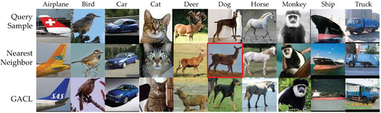
Figure 4. The most confident samples for the query images on STL-10.

4.6.2. Visualization on Classification Results

Following [42], we evaluated our method to obtain extra insight by investigating both successful and failure cases. We studied three cases for each one of four categories from STL-10: (1) success cases, wherein samples are correctly assigned to a target class; (2) false-negative failure cases, wherein samples of a target class are misassigned to other classes with high probability; and (3) false-positive failure cases, where, in terms of a target class, samples of other classes are wrongly assigned to this class with high probability. As shown in Figure 5, GACL can keenly capture the common characteristics between the same categories. For false-negative failure cases, our method mostly fails in isolated samples. It can be observed that the foreground and background interferences in the failed sample are very large, resulting in rarely close neighbors in the dataset, which greatly affects our model. The question of how to distinguish false-positive failure cases in a fine-grained manner is still unresolved.

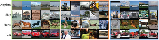
Figure 5. Cases studies of four classes on STL-10. (Left) Successful cases, (Middle) false-negative cases, and (Right) false-positive failure cases.

5. Conclusions

In this paper, we propose a novel graph attention contrastive learning framework (GACL). Different from previous methods that only use pairwise semantic samples, GACL provides a novel mechanism for insight, in which semantic instance-level pairs can be extended to graph-level pairs to supervise the clustering assignment. The designed graph attention mechanism is applied to focus on more undiscovered semantic pairs. Instance-level and graph-level contrastive losses are adopted to learn cluster-friendly representations and compact cluster assignments. Experimental results on real-world datasets demonstrate that our method achieves significant performance gains compared to state-of-the-art methods. In the future, we will apply our method to more relevant directions, such as domain adaptation.

References

- Xie, Y.; Chen, T.; Pu, T.; Wu, H.; Lin, L. Adversarial Graph Representation Adaptation for Cross-Domain Facial Expression Recognition. In Proceedings of the The 28th ACM International Conference on Multimedia, Virtual Event/Seattle, WA, USA, 12–16 October 2020; Chen, C.W., Cucchiara, R., Hua, X., Qi, G., Ricci, E., Zhang, Z., Zimmermann, R., Eds.; ACM International: New York, NY, USA, 2020; pp. 1255–1264. [Google Scholar]
- Luo, Y.; Huang, Z.; Wang, Z.; Zhang, Z.; Baktashmotlagh, M. Adversarial Bipartite Graph Learning for Video Domain Adaptation. In Proceedings of the The 28th ACM International Conference on Multimedia, Virtual Event/Seattle, WA, USA, 12–16 October 2020; Chen, C.W., Cucchiara, R., Hua, X., Qi, G., Ricci, E., Zhang, Z., Zimmermann, R., Eds.; ACM International: New York, NY, USA, 2020; pp. 19–27. [Google Scholar]
- Wang, C.; Li, L.; Zhang, H.; Li, D. Quaternion-based knowledge graph neural network for social recommendation. Knowl. Based Syst. 2022, 257, 109940. [Google Scholar] [CrossRef]
- Thota, M.; Leontidis, G. Contrastive Domain Adaptation. In Proceedings of the IEEE Conference on Computer Vision and Pattern Recognition Workshops, CVPR Workshops 2021, Virtual, 19–25 June 2021; Computer Vision Foundation/IEEE: Nashville, TN, USA, 2021; pp. 2209–2218. [Google Scholar]
- Kang, G.; Jiang, L.; Yang, Y.; Hauptmann, A.G. Contrastive Adaptation Network for Unsupervised Domain Adaptation. In Proceedings of the IEEE Conference on Computer Vision and Pattern Recognition, CVPR 2019, Long Beach, CA, USA, 16–20 June 2019; Computer Vision Foundation/IEEE: Long Beach, CA, USA, 2019; pp. 4893–4902. [Google Scholar]
- Mekhazni, D.; Dufau, M.; Desrosiers, C.; Pedersoli, M.; Granger, E. Camera Alignment and Weighted Contrastive Learning for Domain Adaptation in Video Person ReID. In Proceedings of the IEEE/CVF Winter Conference on Applications of Computer Vision, WACV 2023, Waikoloa, HI, USA, 2–7 January 2023; pp. 1624–1633. [Google Scholar]
- MacQueen, J. Some methods for classification and analysis of multivariate observations. In Fifth Berkeley Symposium on Mathematical Statistics and Probability; University of California: Los Angeles, CA, USA, 1967; pp. 281–297. [Google Scholar]
- Shi, J.; Malik, J. Normalized Cuts and Image Segmentation. IEEE Trans. Pattern Anal. Mach. Intell. 2000, 22, 888–905. [Google Scholar]
- Li, X.; Zhang, R.; Wang, Q.; Zhang, H. Autoencoder Constrained Clustering With Adaptive Neighbors. IEEE Trans. Neural Netw. Learn. Syst. 2020, 32, 443–449. [Google Scholar] [CrossRef] [PubMed]
- Xie, J.; Girshick, R.B.; Farhadi, A. Unsupervised Deep Embedding for Clustering Analysis. In Proceedings of the 2016 International Conference on Machine Learning, New York, NY, USA, 19–24 June 2016; pp. 478–487. [Google Scholar]
- Yang, J.; Parikh, D.; Batra, D. Joint Unsupervised Learning of Deep Representations and Image Clusters. In Proceedings of the 2016 Conference on Computer Vision and Pattern Recognition, Las Vegas, NV, USA, 26 June–1 July 2016; pp. 5147–5156. [Google Scholar]
- Caron, M.; Bojanowski, P.; Joulin, A.; Douze, M. Deep Clustering for Unsupervised Learning of Visual Features. In Proceedings of the 15th European Conference on Computer Vision, 8–14 September 2018; Ferrari, V., Hebert, M., Sminchisescu, C., Weiss, Y., Eds.; Springer: Munich, Germany, 2018; pp. 139–156. [Google Scholar]
- He, K.; Fan, H.; Wu, Y.; Xie, S.; Girshick, R. Momentum contrast for unsupervised visual representation learning. In Proceedings of the 2020 Conference on Computer Vision and Pattern Recognition, Seattle, WA, USA, 14–19 June 2020; pp. 9729–9738. [Google Scholar]
- Chen, T.; Kornblith, S.; Norouzi, M.; Hinton, G.E. A Simple Framework for Contrastive Learning of Visual Representations. In Proceedings of the 2020 International Conference on Machine Learning, Virtual, 12–18 July 2020; pp. 1597–1607. [Google Scholar]
- Li, Y.; Hu, P.; Liu, J.Z.; Peng, D.; Zhou, J.T.; Peng, X. Contrastive Clustering. In Proceedings of the 2021 AAAI Conference on Artificial Intelligence, Virtually, 2–9 February 2021; pp. 8547–8555. [Google Scholar]
- Ji, X.; Vedaldi, A.; Henriques, J.F. Invariant Information Clustering for Unsupervised Image Classification and Segmentation. In Proceedings of the 2019 International Conference on Computer Vision, Seoul, Republic of Korea, 27 October–2 November 2019; pp. 9864–9873. [Google Scholar]
- Wu, J.; Long, K.; Wang, F.; Qian, C.; Li, C.; Lin, Z.; Zha, H. Deep Comprehensive Correlation Mining for Image Clustering. In Proceedings of the 2019 International Conference on Computer Vision, Seoul, Republic of Korea, 27 October–2 November 2019; pp. 8149–8158. [Google Scholar]
- Dang, Z.; Deng, C.; Yang, X.; Wei, K.; Huang, H. Nearest Neighbor Matching for Deep Clustering. In Proceedings of the IEEE Conference on Computer Vision and Pattern Recognition Workshops, CVPR Workshops 2021, Virtual, 19–25 June 2021; pp. 13693–13702. [Google Scholar]
- Van Gansbeke, W.; Vandenhende, S.; Georgoulis, S.; Proesmans, M.; Van Gool, L. Scan: Learning to classify images without labels. In Proceedings of the 2020 European Conference on Computer Vision, Glasgow, UK, 23–28 August 2020; pp. 268–285. [Google Scholar]
- Yang, B.; Fu, X.; Sidiropoulos, N.D.; Hong, M. Towards K-means-friendly Spaces: Simultaneous Deep Learning and Clustering. In Proceedings of the 2017 International Conference on Machine Learning, Sydney, Australia, 6–11 August 2017; pp. 3861–3870. [Google Scholar]
- Wang, C.; Pan, S.; Hu, R.; Long, G.; Jiang, J.; Zhang, C. Attributed Graph Clustering: A Deep Attentional Embedding Approach. In Proceedings of the Twenty-Eighth International Joint Conference on Artificial Intelligence, IJCAI 2019, Macao, China, 10–16 August 2019; Kraus, S., Ed.; Elsevier: Macao, China, 2019; pp. 3670–3676. [Google Scholar]
- Bo, D.; Wang, X.; Shi, C.; Zhu, M.; Lu, E.; Cui, P. Structural Deep Clustering Network. In Proceedings of the WWW ’20: The Web Conference 2020, Taipei, Taiwan, 20–24 April 2020; Huang, Y., King, I., Liu, T., van Steen, M., Eds.; ACM: Taipei, Taiwan, 2020; pp. 1400–1410. [Google Scholar]
- Tu, W.; Zhou, S.; Liu, X.; Guo, X.; Cai, Z.; Zhu, E.; Cheng, J. Deep Fusion Clustering Network. In Proceedings of the Thirty-Fifth AAAI Conference on Artificial Intelligence the Thirty-Third Conference on Innovative Applications of Artificial Intelligence The Eleventh Symposium on Educational Advances in Artificial Intelligence Sponsored by the Association for the Advancement of Artificial Intelligence, Virtually, 2–9 February 2021; AAAI: New York, NY, USA, 2021; pp. 9978–9987. [Google Scholar]
- Peng, Z.; Liu, H.; Jia, Y.; Hou, J. Attention-driven Graph Clustering Network. In Proceedings of the MM ’21: ACM Multimedia Conference, Virtual Event, China, 20–24 October 2021; Shen, H.T., Zhuang, Y., Smith, J.R., Yang, Y., César, P., Metze, F., Prabhakaran, B., Eds.; ACM: New York, NY, USA, 2021; pp. 935–943. [Google Scholar]
- Pan, S.; Hu, R.; Fung, S.; Long, G.; Jiang, J.; Zhang, C. Learning Graph Embedding With Adversarial Training Methods. IEEE Trans. Cybern. 2020, 50, 2475–2487. [Google Scholar] [CrossRef] [PubMed]
- Pan, S.; Hu, R.; Long, G.; Jiang, J.; Yao, L.; Zhang, C. Adversarially Regularized Graph Autoencoder for Graph Embedding. In Proceedings of the Twenty-Seventh International Joint Conference on Artificial Intelligence, IJCAI 2018, Stockholm, Sweden, 13–19 July 2018; Lang, J., Ed.; Elsevier: Stockholm, Sweden, 2018; pp. 2609–2615. [Google Scholar]
- Tao, Z.; Liu, H.; Li, J.; Wang, Z.; Fu, Y. Adversarial Graph Embedding for Ensemble Clustering. In Proceedings of the Twenty-Eighth International Joint Conference on Artificial Intelligence, IJCAI 2019, Macao, China, 10–16 August 2019; Kraus, S., Ed.; Elsevier: Macao, China, 2019; pp. 3562–3568. [Google Scholar]
- Cui, G.; Zhou, J.; Yang, C.; Liu, Z. Adaptive Graph Encoder for Attributed Graph Embedding. In Proceedings of the KDD ’20: The 26th ACM SIGKDD Conference on Knowledge Discovery and Data Mining, Virtual Event, CA, USA, 23–27 August 2020; Gupta, R., Liu, Y., Tang, J., Prakash, B.A., Eds.; ACM: New York, NY, USA, 2020; pp. 976–985. [Google Scholar]
- Liu, L.; Kang, Z.; Ruan, J.; He, X. Multilayer graph contrastive clustering network. Inf. Sci. 2022, 613, 256–267. [Google Scholar] [CrossRef]
- Xia, W.; Gao, Q.; Yang, M.; Gao, X. Self-supervised Contrastive Attributed Graph Clustering. arXiv 2021, arXiv:2110.08264. [Google Scholar]
- Wang, C.; Pan, S.; Long, G.; Zhu, X.; Jiang, J. MGAE: Marginalized Graph Autoencoder for Graph Clustering. In Proceedings of the 2017 ACM on Conference on Information and Knowledge Management, CIKM 2017, Singapore, 6–10 November 2017; Lim, E., Winslett, M., Sanderson, M., Fu, A.W., Sun, J., Culpepper, J.S., Lo, E., Ho, J.C., Donato, D., Agrawal, R., et al., Eds.; ACM: New York, NY, USA, 2017; pp. 889–898. [Google Scholar]
- Kipf, T.N.; Welling, M. Variational Graph Auto-Encoders. arXiv 2016, arXiv:1611.07308. [Google Scholar]
- Cheng, J.; Wang, Q.; Tao, Z.; Xie, D.; Gao, Q. Multi-View Attribute Graph Convolution Networks for Clustering. In Proceedings of the Twenty-Ninth International Joint Conference on Artificial Intelligence, IJCAI, Yokohama, Japan, 11–17 July 2020; Bessiere, C., Ed.; Elsevier: Yokohama, Japan, 2020; pp. 2973–2979. [Google Scholar]
- Vaswani, A.; Shazeer, N.; Parmar, N.; Uszkoreit, J.; Jones, L.; Gomez, A.N.; Kaiser, L.; Polosukhin, I. Attention is All you Need. In Proceedings of the Advances in Neural Information Processing Systems 30: Annual Conference on Neural Information Processing Systems 2017, Long Beach, CA, USA, 4–9 December 2017; Guyon, I., von Luxburg, U., Bengio, S., Wallach, H.M., Fergus, R., Vishwanathan, S.V.N., Garnett, R., Eds.; MIT: Long Beach, CA, USA, 2017; pp. 5998–6008. [Google Scholar]
- Park, J.; Lee, M.; Chang, H.J.; Lee, K.; Choi, J.Y. Symmetric Graph Convolutional Autoencoder for Unsupervised Graph Representation Learning. In Proceedings of the 2019 International Conference on Computer Vision, Seoul, Republic of Korea, 27 October–2 November 2019; pp. 6518–6527. [Google Scholar]
- Zhang, X.; Liu, H.; Li, Q.; Wu, X. Attributed Graph Clustering via Adaptive Graph Convolution. In Proceedings of the Twenty-Eighth International Joint Conference on Artificial Intelligence, IJCAI 2019, Macao, China, 10–16 August 2019; Kraus, S., Ed.; Elsevier: Macao, China, 2019; pp. 4327–4333. [Google Scholar]
- Hadsell, R.; Chopra, S.; LeCun, Y. Dimensionality Reduction by Learning an Invariant Mapping. In Proceedings of the EEE Computer Society Conference on Computer Vision and Pattern Recognition, New York, NY, USA, 17–22 June 2006; pp. 1735–1742. [Google Scholar]
- Sharma, V.; Tapaswi, M.; Sarfraz, M.S.; Stiefelhagen, R. Clustering based Contrastive Learning for Improving Face Representations. In Proceedings of the 2020 15th IEEE International Conference on Automatic Face and Gesture Recognition (FG 2020), Buenos Aires, Argentina, 16–20 November 2020; pp. 109–116. [Google Scholar]
- Dosovitskiy, A.; Springenberg, J.T.; Riedmiller, M.A.; Brox, T. Discriminative Unsupervised Feature Learning with Convolutional Neural Networks. In Proceedings of the Annual Conference on Neural Information Processing Systems 2014, Montreal, QC, Canada, 8–13 December 2014; pp. 766–774. [Google Scholar]
- Chang, J.; Wang, L.; Meng, G.; Xiang, S.; Pan, C. Deep Adaptive Image Clustering. In Proceedings of the International Conference on Computer Vision, Venice, Italy, 17–31 July 2017; pp. 5880–5888. [Google Scholar]
- Schroff, F.; Kalenichenko, D.; Philbin, J. FaceNet: A unified embedding for face recognition and clustering. In Proceedings of the IEEE Conference on Computer Vision and Pattern Recognition (CVPR), Boston, MA, USA, 7–12 June 2015; pp. 815–823. [Google Scholar]
- Huang, J.; Gong, S.; Zhu, X. Deep Semantic Clustering by Partition Confidence Maximisation. In Proceedings of the IEEE Conference on Computer Vision and Pattern Recognition, Boston, MA, USA, 7–12 June 2020; pp. 8846–8855. [Google Scholar]
- Krizhevsky, A.; Hinton, G. Learning Multiple Layers of Features from Tiny Images. 2009. Available online: http://www.cs.utoronto.ca/~kriz/learning-features-2009-TR.pdf (accessed on 8 April 2009).
- Coates, A.; Ng, A.Y.; Lee, H. An Analysis of Single-Layer Networks in Unsupervised Feature Learning. In Proceedings of the International Conference on Artificial Intelligence and Statistics, Fort Lauderdale, FL, USA, 11–13 April 2011; Gordon, G.J., Dunson, D.B., Dudík, M., Eds.; AISTATS: Fort Laud- erdale, FL, USA, 2011; pp. 215–223. [Google Scholar]
- Le, Y.; Yang, X. Tiny imagenet visual recognition challenge. CS 231N 2015, 7, 3. [Google Scholar]
- Gowda, K.C.; Krishna, G. Agglomerative clustering using the concept of mutual nearest neighbourhood. Pattern Recognit. 1978, 10, 105–112. [Google Scholar] [CrossRef]
- Cai, D.; He, X.; Wang, X.; Bao, H.; Han, J. Locality Preserving Nonnegative Matrix Factorization. In Proceedings of the International Joint Conference on Artificial Intelligence, Pasadena, CA, USA, 11–17 July 2009; Boutilier, C., Ed.; Elsevier: Pasadena, CA, USA, 2009; pp. 1010–1015. [Google Scholar]
- Bengio, Y.; Lamblin, P.; Popovici, D.; Larochelle, H. Greedy Layer-Wise Training of Deep Networks. In Proceedings of the Annual Conference on Neural Information Processing Systems, Vancouver, BC, Canada, 4–7 December 2006; Schölkopf, B., Platt, J.C., Hofmann, T., Eds.; MIT: Vancouver, BC, Canada, 2006; pp. 153–160. [Google Scholar]
- Radford, A.; Metz, L.; Chintala, S. Unsupervised Representation Learning with Deep Convolutional Generative Adversarial Networks. In Proceedings of the International Conference on Learning Representations, San Juan, Puerto Rico, 2–4 May 2016. [Google Scholar]
- Zeiler, M.D.; Krishnan, D.; Taylor, G.W.; Fergus, R. Deconvolutional networks. In Proceedings of the 2020 Conference on Computer Vision and Pattern Recognition, Seattle, WA, USA, 14–19 June 2020; pp. 2528–2535. [Google Scholar]
- Kingma, D.P.; Welling, M. Auto-Encoding Variational Bayes. In Proceedings of the International Conference on Learning Representations, Banff, AB, Canada, 14–16 April 2014. [Google Scholar]
- Dang, Z.; Deng, C.; Yang, X.; Huang, H. Doubly Contrastive Deep Clustering. arXiv 2021, arXiv:2103.05484. [Google Scholar]
- Zhong, H.; Wu, J.; Chen, C.; Huang, J.; Deng, M.; Nie, L.; Lin, Z.; Hua, X. Graph Contrastive Clustering. arXiv 2021, arXiv:2104.01429. [Google Scholar]
Disclaimer/Publisher’s Note: The statements, opinions and data contained in all publications are solely those of the individual author(s) and contributor(s) and not of MDPI and/or the editor(s). MDPI and/or the editor(s) disclaim responsibility for any injury to people or property resulting from any ideas, methods, instructions or products referred to in the content. |
© 2023 by the authors. Licensee MDPI, Basel, Switzerland. This article is an open access article distributed under the terms and conditions of the Creative Commons Attribution (CC BY) license (https://creativecommons.org/licenses/by/4.0/).