Novelty Detection and Fault Diagnosis Method for Bearing Faults Based on the Hybrid Deep Autoencoder Network

Abstract

In the event of mechanical equipment failure, the fault may not belong to any known category, and existing deep learning methods often misclassify such faults into a known class, leading to erroneous fault diagnosis. In order to address the challenge of identifying new types of faults in mechanical equipment fault diagnosis, this paper proposes a novelty detection and fault diagnosis method for bearing faults based on a hybrid deep autoencoder network. Firstly, a hybrid deep autoencoder network with one input and two outputs was constructed. The original data were then fed into the network to obtain its low-dimensional representation and reconstructed data. By setting a threshold based on the reconstruction error, novel class faults can be detected, while known faults can be classified based on low-dimensional features. Experimental results demonstrate that the proposed method achieves a recognition accuracy of 98.59% (100%) for novel class identification (known fault classification) on the CWRU bearing dataset, 96.79% (98.53%) on the Paderborn dataset, and 84.34% (97.03%) on the MFPT dataset. Therefore, the hybrid deep autoencoder network not only accurately detects unknown types of faults but also effectively classifies known fault types, demonstrating excellent fault identification and classification capabilities.

1. Introduction

Bearings are critical components of modern mechanical equipment that serve to support and reduce friction in rotating shafts. During the operation of equipment, bearings can suffer from various forms of damage, such as detachment, wear, and deformation [1]. The proper functioning of bearings directly impacts the overall performance of the entire machinery. Therefore, real-time and accurate diagnosis of bearing conditions is of great significance to ensure the reliable operation of mechanical equipment. In the past, bearing fault detection relied mainly on manual inspection, which was not only time-consuming but also costly. With the rapid development of deep neural networks, methods based on deep learning have become a research focus in the field of fault diagnosis. Utilizing deep learning methods for fault diagnosis can greatly enhance the efficiency of fault detection and diagnosis.

In recent years, the significant improvement in computer performance and the rapid development of sensor technology have driven the application of deep learning methods in the field of fault diagnosis. Deep learning, with its powerful adaptive capabilities, automatically extracts fault features for fault diagnosis. Compared to traditional methods, deep learning eliminates the need for manual feature extraction, reducing the reliance on expert knowledge in fault diagnosis. Consequently, deep learning has become the preferred approach for mechanical equipment fault diagnosis. Numerous researchers have achieved high-precision fault classification using various deep learning methods. For example, Saufi et al. [2] improved the deep sparse autoencoder network for the fault diagnosis of mechanical components, achieving higher diagnostic accuracy on different datasets. While these methods accurately classify known types of fault data, they often overlook the detection of unknown faults, also known as novel faults. Most fault diagnosis methods that are currently available lack the ability to identify novel faults, resulting in the misclassification of these data into known categories, which introduces errors and hinders further analysis. Asavalertpalakorn et al. [3] used long short-term memory (LSTM) autoencoders to detect novel faults in bearing data, but they were unable to classify known faults. There are numerous deep learning methods applied in the field of fault diagnosis, with some achieving high-precision classification of fault types, and others focusing on novel fault detection. However, there is a lack of methods that simultaneously address novel fault detection and known fault classification, which is essential for practical industrial requirements. Yang et al. [4] designed a deep neural network based on sparse autoencoders (SAE) that successfully recognizes novel faults and classifies known faults. However, this method requires a large number of training samples to achieve high-precision classification; further improvements in accuracy are still necessary.

In order to address these challenges, this paper proposes a novel detection and fault diagnosis method for bearing faults based on a hybrid deep autoencoder network. This method combines the unsupervised training characteristics of autoencoders and utilizes unsupervised learning to train the network model. Additionally, it leverages a small amount of labeled data to train the classifier, reducing the reliance on labeled data for fault diagnosis. This approach effectively resolves the contradiction between limited fault data samples and the extensive training requirements of deep learning models. By setting a threshold based on the reconstruction data, it achieves novel class fault recognition in bearings, thereby addressing the difficulty of identifying new faults in mechanical equipment fault diagnosis and significantly improving the accuracy of bearing fault recognition. The proposed method achieves a detection score of 0.98 on the Case Western Reserve University (CWRU) bearing dataset, which is 0.23 higher than the approach based on the LSTM autoencoder network for novel class recognition and fault diagnosis, and is 0.05 higher than the SAE network-based method. On the German Paderborn dataset, the detection score is 0.94, which is 0.31 higher than the LSTM model and 0.03 higher than the SAE model. On the Mechanical Fault Prevention Technology Association (MFPT) dataset, the detection score is 0.92, which is 0.21 higher than the LSTM model and 0.03 higher than the SAE model. Compared to existing methods, the proposed method demonstrates improvements in both novel fault detection and known fault classification accuracy.

In summary, the main contributions of this paper are as follows:

(1)

This paper designs a hybrid deep autoencoder network composed of the convolutional autoencoder, new-fault detector, and classifier. It achieves the functionality of detecting novel faults and classifying known faults. By setting a threshold based on reconstruction errors, the proposed method automatically determines whether a fault belongs to unknown faults, thereby addressing the issue of misclassifying unknown faults as known faults.

(2)

This method employs unsupervised training of the hybrid deep autoencoder network using data from known fault classes to obtain reconstruction data and low-dimensional features of the samples. Additionally, it utilizes a small amount of labeled data for supervised training of the network. This approach accelerates the training speed of the network and reduces the required sample size for training.

(3)

Through comparisons with LSTM and SAE models, in terms of novel fault recognition performance and fault classification, it is demonstrated that the proposed model performs well in both novel fault detection and known fault classification. Experimental results show that the overall detection performance of the hybrid deep autoencoder network model is superior to other models, with higher detection results on all three datasets. This confirms the effectiveness of the proposed method.

The rest of the paper is organized as follows. Section 2 provides an overview of recent research in the field of mechanical equipment fault diagnosis. Section 3 presents a detailed description of the proposed fault diagnosis model and method. Section 4 outlines the experimental details. Finally, conclusions are drawn in Section 5.

2. Related Work

With the rapid development of deep neural networks, various deep learning methods have been extensively applied in fault recognition and diagnosis, enabling intelligent fault diagnosis of mechanical equipment [5,6,7,8,9,10]. Deep autoencoder networks, characterized by their symmetric structure, have been widely employed in fault classification due to their unsupervised learning approach that adaptively extracts features from complex objects. Lu et al. [11] proposed a fault diagnosis method for rolling bearings based on LSTM autoencoders, which automatically learn useful features from vibration signals. Fu-Lin et al. [12] combined simulation and time-frequency analysis methods to study the application of autoencoders in bearing fault diagnosis, resulting in stable diagnostic outcomes. Xu et al. [13] introduced an improved stacked denoising autoencoder method for fault diagnosis of metro traction motor bearings, effectively extracting deep features even under complex operating conditions. Lu et al. [14] utilized deep autoencoders to learn and extract fault data features, followed by the use of a Softmax classifier for fault classification. Saufi et al. [2] improved deep sparse autoencoders for the fault diagnosis of mechanical components. In summary, deep autoencoder networks have demonstrated their strength in unsupervised training and deep feature extraction, reducing the reliance on labeled samples and enhancing diagnostic accuracy in small-sample fault diagnosis methods. A convolutional neural network (CNN) is widely regarded for its strong feature extraction capability, making it crucial in the field of fault classification [15,16,17,18,19,20]. Guo et al. [21] combined CNN to extract and analyze features from speed signals, proposing a bearing fault diagnosis method based on motor speed signals. Xu et al. [22] introduced an improved deep CNN fault diagnosis model, achieving high-precision fault diagnosis even in noisy environments. Zhang et al. [23] transformed the original signal into two-dimensional images for feature extraction, eliminating the influence of manual feature engineering; they made improvements to the CNN network for feature extraction and fault diagnosis processes. Hence, the powerful feature extraction capability of CNN enables us to extract key information more efficiently, leading to improved detection accuracy and faster network training speed. Combining the unsupervised learning ability of deep autoencoders and the excellent feature extraction capability of convolutional neural networks, various convolutional autoencoder networks have been widely proposed and applied in the field of fault diagnosis [24,25,26,27,28]. Song et al. [29] proposed a combined model of stacked denoising autoencoder and CNN for fault diagnosis of wind turbine bearings, which improved the accuracy of fault diagnosis. Wu et al. [30] introduced a semi-supervised fault diagnosis method based on convolutional autoencoders, enhancing the network with CNN structures to handle more complex data. They achieved high diagnostic accuracy on motor bearings and industrial water turbine datasets. Furthermore, these deep learning methods have also been applied in other domains, such as the prediction of mechanical equipment lifespan [31,32,33].

In the past few years, many novelty detection methods have been proposed. Del Buono et al. [34] conducted a comparison of machine learning and deep learning methods for novelty detection, evaluating their effectiveness and efficiency across different scenarios. The experimental results demonstrated the superiority of deep learning methods over traditional machine learning methods. Wu et al. [35] introduced a Transformer-based classifier for novelty detection, utilizing Mahalanobis distance to detect novel faults. Yang et al. [4] designed a deep neural network based on sparse autoencoders, achieving recognition of novel faults and classification of known faults. Sun et al. [36] employed a one-class support vector machine (OC-SVM) to separate noise-contaminated voice samples, achieving the separation of two types of sound signals. Li et al. [37] proposed a fault detection method based on the support vector machine (SVM) observer, realizing the novelty detection of astronomical telescope drive systems. Górski et al. [38] designed a detection system for parallel gearboxes, comparing various rotating machinery fault novelty detection methods and validating their effectiveness on the gearbox dataset through experiments. The aforementioned methods have important theoretical implications for our research.

3. Novelty Detection and Fault Diagnosis Method Based on a Hybrid Deep Autoencoder Network

In this section, a novel method for novelty detection and fault diagnosis of bearing faults based on a hybrid deep autoencoder is proposed. This method enables fault classification and can detect unknown faults that have not previously occurred in the equipment.

3.1. Network Structure

The model consists of four modules: encoder, decoder, detector, and classifier, as shown in Figure 1. The encoder is used to obtain the hidden layer features z of the input data, which are then passed to the decoder to reconstruct the data. The detector examines the reconstruction results from the decoder to detect whether it belongs to a new fault, while the classifier analyzes the hidden features z to obtain the fault classification results.

3.1.1. Encoder

The encoder’s purpose is to extract compressed representations and hidden features of the input data. In this paper, the proposed encoder comprises four convolutional layers and two fully connected layers. The convolution operation, which is crucial for the success of CNN, ensures high computational efficiency and robustness through sparse interaction and weight-sharing strategies. Each convolutional layer has a kernel size of 3 × 3, a stride of 2, and a padding of 1 to achieve downsampling and obtain the compressed representation of the image. The convolution operation can be expressed as follows:

$$X^L=\sum _{j=1}^m{f}_j\left(\sum _{i=1}^I{W}_{i,j}^{L-1}·X_{i,j}^{L-1}+b_j^{L-1}\right)$$

(1)

In Equation (1), $X^L$ is the output of the convolution layer of the Lth layer, · represents the convolution operation, $X_{i,j}^L$ is the ith feature map of the Lth layer of the jth channel (a total of I feature inputs), $W_{i,j}^L$ and $b_j^L$ are the convolution kernel and bias vector of the Lth layer of the jth channel, respectively, f is the activation function of the layer, and m is the number of channels.

With each convolutional layer, the size of the input image is reduced by half. After four layers of convolutional operations, the input image of size 64 × 64 is compressed into a feature map of size 4 × 4. A ‘flatten’ layer is inserted after the final convolutional layer to act as a bridge between the convolutional and fully connected layers. The flattening layer flattens the compressed feature map into one-dimensional data and serves as the input layer to the fully connected layer. The fully connected layer comprises two layers, with 64 and 32 neurons, respectively. In the fully connected layer, each neuron node in layer L-1 is connected to every neuron node in layer L, and the mathematical expression is as follows.

$$y^L=f\left(W^L{X}^{L-1}+b^L\right)$$

(2)

In Equation (2), $X^{L-1}$ and $y^L$ are the input and output of layer L, $W^L$ and $b^L$ are the weight and bias, and f is the activation function.

The rectified linear unit (ReLU) activation function is used in all hidden layers of the encoder.

3.1.2. Decoder

The decoder is the inverse operation of the encoder, used to reconstruct the input data. The network layers and neuron quantities of the decoder are designed to be symmetrical to the encoder, including two fully connected layers and four deconvolutional layers. Deconvolutional operations are used for upsampling the image, increasing its size, so that the reconstructed image outputted by the decoder is the same size as the original image. We still use ReLU as the activation function for all hidden layers in the decoder, and employ techniques such as batch normalization (BN) to improve overfitting issues. The output of the decoder has the same size as the original data, allowing for the calculation of reconstruction errors. The structural details of the encoder and decoder are shown in Figure 2.

3.1.3. Detector

The task of the detector is to determine whether the tested data belong to a new fault. During the detection process, the recognition of new faults is achieved by comparing the reconstruction error of the tested sample with a predefined threshold. The autoencoder network is trained only on normal conditions and known fault conditions. Therefore, when the tested data belong to normal conditions or known faults, the network can reconstruct the original image well. However, when the tested data belong to an unknown fault (new fault), the network still relies on the feature space of the training samples for reconstruction, resulting in reconstruction errors deviating from the original distribution range, causing the reconstruction error greater than the predefined threshold.

The reconstruction error is calculated using the binary cross-entropy loss formula shown in Equation (3). Then, all the reconstruction errors are saved into an error list, obtaining the error distribution of the training samples.

$$e=-\frac{1}{m}\sum _{i=1}^m[x_{i}log{\widehat{x}}_i+(1-x_i)log(1-x_i)]$$

(3)

where $x_i$ represents the input data during training, and ${\widehat{x}}_i$ represents the corresponding reconstructed data.

After calculating the error distribution between the original data and the reconstructed data for the known fault class, the threshold is set using the boxplot method. The schematic diagram for selecting the threshold using the boxplot method is shown in Figure 3. The maximum value, upper quartile, median, lower quartile, and minimum value are used to describe the data distribution of the errors, thereby identifying outliers.

The upper bound is used as the detection threshold for new faults. The expression for $\delta$ is as follows:

$$\delta =Q3+1.5(Q3-Q1)$$

(4)

In Equation (4), $Q1$ represents the lower quartile of the reconstruction error of the training data, which is the 25th percentile, and $Q3$ represents the upper quartile of the reconstruction error, which is the 75th percentile.

When the reconstruction error of the tested sample is greater than this threshold, it indicates the presence of a new fault in the device. The output of the detector can be represented as follows:

$$Output=\left\{\begin{array}{cc}Newfaults,\hfill & e^{TEST}>\delta \hfill \\ Normalorknownfaults,\hfill & e^{TEST}\le \delta \hfill \end{array}\right.$$

(5)

3.1.4. Classifier

The classifier is a Softmax classification layer commonly used to solve multi-class classification problems. It maps the hidden features outputted by the encoder to values between [0, 1], and ensures that the sum of all values is equal to 1. This allows for direct output of the probabilities of different classes, enabling fault-type classification. The Softmax structure diagram is shown in Figure 4.

Given the labeled data samples as $(x^{\left(1\right)},y^{\left(1\right)})$, $(x^{\left(2\right)},y^{\left(2\right)})$, …, $(x^{\left(n\right)},y^{\left(n\right)})$, $y^{\left(i\right)}\in \{1,2,3,\dots ,C\}$, where C represents the label categories. For each $x^{\left(i\right)}$, the hypothetical output value obtained after passing through the Softmax function is as follows:

$$h\left(x^{\left(i\right)}\right)=\frac{e^{x^{\left(i\right)}}}{{\sum }_{j=1}^C{e}^{x^{\left(i\right)}}}$$

(6)

Based on Equation (6), the probability value of each kind of label $p(y^{\left(i\right)}=C|x^{\left(i\right)})$ is estimated, and the sum of all probabilities of $h\left(x^{\left(i\right)}\right)$ is equal to 1. For each feature vector $x^{\left(i\right)}$, the corresponding probability vector P can be obtained:

$$P=h_{\theta }\left(x^{\left(i\right)}\right)=\left[\begin{array}{c}p(y^{\left(i\right)}=1|x^{\left(i\right)};\theta )\\ p(y^{\left(i\right)}=2|x^{\left(i\right)};\theta )\\ \dots \\ p(y^{\left(i\right)}=C|x^{\left(i\right)};\theta )\end{array}\right]=\frac{1}{{\sum }_{j=1}^C{e}^{{\theta }_j^T{x}^{\left(i\right)}}}\left[\begin{array}{c}{e}^{{\theta }_1^T{x}^{\left(i\right)}}\\ e^{{\theta }_2^T{x}^{\left(i\right)}}\\ \dots \\ e^{{\theta }_C^T{x}^{\left(i\right)}}\end{array}\right]$$

(7)

In Equation (7), $\theta ={\left[{\theta }_1,{\theta }_2,\dots ,{\theta }_C\right]}^T$ is the weight matrix between the feature space and the Softmax classification layer, and ${\theta }_j$ represents the weight vector corresponding to the feature vector $x^{\left(i\right)}$ and the jth label in the Softmax layer.

The Softmax classifier can calculate the feature vector $x^{\left(i\right)}$ through a series of calculations to obtain the probability vector P, $P=\left\{P_1,P_2,\dots ,P_C\right\}$. When there is a maximum $P_k$ in P, it is considered that the feature vector $x^{\left(i\right)}$ represents the kth class label, $k=1,2,\dots ,C$.

In the proposed network structure, the Softmax layer includes C neurons corresponding to C known types of faults.

In general, the model primarily consists of four components: encoder, decoder, detector, and classifier. The encoder and decoder exhibit a symmetrical structure, the detector is a custom function that compares the output of the decoder with a threshold, and the classifier is a Softmax layer with C neurons. In order to provide a clear understanding of the specific features and components of our proposed model, we have detailed the number of layers, layer types, and their configurations in

Table 1. Model configuration.

Component	Layer Types	Output Size	Other Parameter Configurations
Encoder	Input layer	(1, 64, 64)
	Convolutional layer	(16, 32, 32)	kernel = 3 × 3, stride = 2, padding = 1
	Convolutional layer	(32, 16, 16)	kernel = 3× 3, stride = 2, padding = 1
	Batch Normalization layer	(32, 16, 16)
	Convolutional layer	(32, 8, 8)	kernel = 3 × 3, stride = 2, padding = 1
	Convolutional layer	(32, 4, 4)	kernel = 3 × 3, stride = 2, padding = 1
	Flatten layer	(512)
	Fully connected layer	(64)
	Fully connected layer	(32)
Decoder	Fully connected layer	(64)
	Flatten layer	(512)
	Unflattened layer	(32, 4, 4)
	Deconvolutional layer	(32, 8, 8)	kernel = 3 × 3, stride = 2, padding = 1
	Deconvolutional layer	(32, 16, 16)	kernel = 3 × 3, stride = 2, padding = 1
	Batch Normalization layer	(32, 16, 16)
	Deconvolutional layer	(16, 32, 32)	kernel = 3 × 3, stride = 2, padding = 1
	Deconvolutional layer	(16, 32, 32)	kernel = 3 × 3, stride = 2, padding = 1
Classifier	Softmax layer	(C)

.

3.2. Loss Function

This paper addresses the issue of reducing reliance on labeled data for fault diagnosis and resolving the conflict between limited fault data and the requirement for extensive sample training in deep learning models. To overcome these challenges, the paper utilizes the unsupervised learning capabilities of autoencoders. By inputting all known fault classes of unlabeled data into the network, the model undergoes unsupervised training. The reconstruction error, measured using the binary cross-entropy loss function ($L_{BCE}$), is used to assess the dissimilarity between the input and output images. Our encoder and decoder primarily use downsampling and upsampling methods. First, downsampling is performed using convolutional operations to compress the image, filtering out less useful and redundant information while retaining the most informative features. Then, upsampling is achieved through the process of deconvolution, reconstructing the compressed feature maps into reconstructed images of the same size as the original image. This process incurs a loss, so while training the network, we continuously minimize the error between the reconstructed images and the original images to reduce the loss caused by downsampling and upsampling methods. In short, the feature extraction training of the hybrid deep autoencoder is accomplished by continuously minimizing the reconstruction error, which is formulated as follows:

$$L_{BCE}=-\frac{1}{m}\sum _{i=1}^m[x_{i}log{\widehat{x}}_i+(1-x_i)log(1-x_i)]$$

(8)

In order to achieve the network’s classification capability for known fault classes, a small amount of labeled data needs to be input into the network for supervised training. The weights and bias vectors of the classifier and encoder are updated, and the cross-entropy loss ($L_{CE}$) is used to calculate the distance between the hidden features and the true labels. The fault classification training of the Softmax classifier is achieved by continuously reducing this distance:

$$L_{CE}=-\frac{1}{m}\left[\sum _{i=1}^m\sum _{j=1}^{C}1\{y^{\left(i\right)}=j\}·log\frac{e^{{\theta }_j^T{x}^{\left(i\right)}}}{{\sum }_{k=1}^C{e}^{{\theta }_k^T{x}^{\left(i\right)}}}\right]$$

(9)

Combining these two loss functions into an overall objective function, the network is trained using gradient descent. Experimental results have shown that this training approach is faster and more versatile than traditional pre-training and fine-tuning methods. The training process is as follows:

$$L=\alpha L_{BCE}+\beta L_{CE}$$

(10)

In Equation (10), $\alpha$ and $\beta$ are weights that adjust the impact of individual losses on the overall objective function. They are hyperparameters that need to be manually set and their optimal values are determined through cross-validation. Additionally, the network is trained with the goal of minimizing the above objective loss functions.

In the process of constructing and training the network architecture, as the depth of the network increases, the training becomes more challenging. Therefore, batch normalization layers are added to the network structure to accelerate training, prevent overfitting, and enhance the model’s generalization performance.

3.3. Diagnostic Process

The proposed hybrid deep autoencoder network learns latent features by reconstructing input data and diagnoses fault types based on these latent features. By learning the reconstruction error distribution of the training data, it can also detect new fault classes. The fault diagnosis process of the hybrid deep autoencoder is illustrated in Figure 5. Firstly, the training samples are input into the hybrid deep autoencoder network for semi-supervised training. The new fault detection threshold is set based on the reconstruction error distribution of the training samples. Then, the test samples are input into the trained network model. Based on the output of the detector, it is determined whether it belongs to a known class. If it does not belong to a known class, it is identified as a new fault class. Otherwise, based on the output of the classifier, the fault class is diagnosed.

4. Experiment

In order to validate the performance of the proposed hybrid deep autoencoder network model, experiments were conducted using three publicly available bearing datasets and compared with similar research methods in recent years.

4.1. Dataset

4.1.1. CWRU Dataset

The CWRU dataset, acquired from the Bearing Data Center at Case Western Reserve University [39], is a widely used open dataset. Our experiments focused on the faulty and normal bearing data, sampled at 12 kHz. The dataset includes three types of faults: inner race fault, outer race fault, and ball fault, with fault diameters of 0.007 inches, 0.014 inches, and 0.021 inches, respectively. Detailed information about the dataset can be found in

Table 2. Fault types of CWRU dataset.

Fault Class	Fault Diameter (inch)	Class Label	Number of Original Data Points	Number of Samples
Normal	/	C1	243,938	238
Inner race fault	0.007	C2	121,265	118
Inner race fault	0.014	C3	121,846	118
Inner race fault	0.021	C4	122,136	119
Balls fault	0.007	C5	122,571	119
Balls fault	0.014	C6	121,846	118
Balls fault	0.021	C7	121,991	119
Outer race fault (at 6 o ’clock)	0.007	C8	121,991	119
Outer race fault (at 6 o ’clock)	0.014	C9	121,846	118
Outer race fault (at 6 o ’clock)	0.021	C10	122,426	119

.

The collected data signals are divided into samples, with each sample consisting of 1024 data points. These segmented samples are then subjected to wavelet transformation. Wavelet transformation is capable of capturing local signal features in both time and frequency domains, allowing for the dynamic adjustment of time and frequency windows based on specific signal shapes. Due to these advantages, wavelet transformation is employed to convert the one-dimensional bearing signal into a two-dimensional time-frequency image, which serves as the source data for training and testing purposes. Figure 6 illustrates the transformed time-frequency image. The number of samples under each category label after segmentation is presented in the last column of Table 2.

Before conducting the experiment, we need to define the training set and the test set based on our research content. In order to test the detection ability of the proposed method for new class faults, we need to assume that some fault types are unknown faults. We assume that classes 1 to 7 represent normal states of the equipment and known fault states of the system, while classes 8 to 10 represent unknown faults that the system is not aware of. We randomly select 70% of the data from each of the known fault categories (classes 1–7) form the training set, and the remaining 30% and all the data from the unknown fault categories (classes 8–10) form the test set. During this process, we need to ensure that the sample data in the training set reflects the distribution characteristics of the entire dataset, and that the training set and the test set are independent of each other.

4.1.2. The Paderborn Dataset

The Paderborn dataset from Germany was collected at a sampling frequency of 64 kHz for bearing fault data [40]. One healthy state vibration data and vibration data from six real damage states were selected as experimental data from this dataset. The damage types for these six fault classes are all “fatigue: pitting”, and the damage characteristics are all “single point”. However, their damage locations, patterns, distribution, and damage degree are all different. The damage conditions are shown in

Table 3. Fault types of the Paderborn dataset.

File Number	Location of Damage	Class	Damage Mode	Mode of Distribution	Degree of Damage
K005	/	C1	/	/	/
KI04	Inner	C2	multiple	no repetition	1
KI14	Inner	C3	multiple	no repetition	1
KI16	Inner	C4	single	no repetition	3
KI17	Inner	C5	single	random	1
KA04	Outer	C6	single	no repetition	1
KA16	Outer	C7	repetitive	random	2

.

Each category includes 256,004 data points. As before, each set of 1024 data points is divided into a sample, with 250 samples per category. Then, each sample is transformed into a 64 × 64 time-frequency image using wavelet transform. Figure 7 shows the time-frequency images for each category. In order to test the proposed method’s ability to detect new class faults, we assume that normal and different degrees of inner ring faults are known faults, while outer ring faults are unknown faults. Only 70% of the data for known faults are used as the training set to train the hybrid deep autoencoder network, while the remaining 30% and the unknown faults are used as the test set. The training set follows the distribution of the samples, and the training set and test set are mutually independent. The network’s ability to detect novelty and classify faults is tested and evaluated on this dataset.

4.1.3. MFPT Dataset

The dataset of the Machinery Failure Prevention Technology Association (MFPT) in the United States includes normal state data, outer race faults, and inner race faults under different sampling rates and loads [41]. A set of vibration signals collected under one type of normal state, four types of outer race faults, and three types of inner race faults were randomly selected as experimental data. The detailed descriptions of each data category are shown in

Table 4. Description of the MFPT dataset.

Type of Fault	Class	Sampling Rate (sps)	Load (Ibs)	Number of Data Points	Sample Size
normal	C1	97,656	270	58,5936	572
Outer	C2	97,656	270	58,5936	572
Outer	C3	48,828	25	146,484	143
Outer	C4	48,828	50	146,484	143
Outer	C5	48,828	100	146,484	143
Inner	C6	48,828	0	146,484	143
Inner	C7	48,828	50	146,484	143
Inner	C8	48,828	100	146,484	143

.

Each category contains tens of thousands of data points. Similar to the two datasets mentioned earlier, signal segmentation and wavelet transform processing are performed, followed by training and testing using time-frequency maps. The initial number of data points and the number of processed samples are also listed in Table 4. The transformed time-frequency maps are shown in Figure 8. We assume that the normal state and outer race faults under different loads are known types of faults, while the inner race faults are considered unknown types of faults. We still only use 70% of the data from known types of faults as the training set to train the hybrid deep autoencoder network, ensuring that the training set follows the sample distribution. The remaining 30% of the known fault classes and the unknown faults are used as the test set to evaluate the model.

4.2. Implementation

The experimental environment for this study consisted of Windows 10, Python 3.9.7, Pytorch 1.13.1. All computations were carried out using an Intel Core i7-10700 CPU and 16 GB RAM.

Prior to training, the input image size was set to 64 × 64. We utilized the Adam optimizer with a learning rate of 0.00005 to train the network. The training process involved 40 epochs, with a weight decay of 0.001. The loss function weights $\alpha$ and $\beta$ were both set to 0.5. After training, we evaluated the novelty detection and fault diagnosis capabilities of the proposed method in this paper. We compared it with the novelty detection and fault diagnosis methods based on the LSTM autoencoder network in reference [3], as well as the novelty detection and fault diagnosis methods based on the sparse autoencoder (SAE) network in reference [4].

4.3. Evaluation Indicators

The main purpose of the experiment is to validate the model’s performance in novel class recognition and fault classification. Therefore, different metrics are set for these two aspects. In the field of novelty detection and anomaly detection, some scholars use the true positive rate ($TPR$) to evaluate the proportion of correctly detected positive samples out of all positive samples, and use the true negative rate ($TNR$) to represent the proportion of correctly detected negative samples out of all negative samples. Here, positive refers to known or normal classes, negative refers to new or abnormal classes, and correct detection is considered true. The $F1$ score combines $TPR$ and $TNR$, and is the main metric for evaluating the model’s performance in novel class detection, ranging from 0 to 1, where a higher value indicates better detection performance. In terms of fault classification performance, accuracy ($ACC$) is commonly used to evaluate the diagnostic accuracy of the model for known faults [42].

In this experiment, the known class is defined as the positive sample, while the unknown or new class is defined as the negative sample. $TP$ (true positive) represents the count of correctly predicted positive samples, $FN$ (false negative) represents the count of incorrectly predicted positive samples, $TN$ (true negative) represents the count of correctly predicted negative samples, and $FP$ (false positive) represents the count of incorrectly predicted negative samples. These metrics are illustrated by Equations (11)–(14).

$$TPR=\frac{TP}{TP+FN}$$

(11)

$$TNR=\frac{TN}{TN+FP}$$

(12)

$$F1=\frac{2TP}{2TP+FP+FN}$$

(13)

$$ACC=\frac{TP+TN}{TP+FN+TN+FP}$$

(14)

4.4. Experimental Results and Analysis

In this study, we evaluated our proposed method from three perspectives: novelty detection, fault classification, and model complexity. In order to showcase the diagnostic performance of our model, we compare it with the LSTM autoencoder model and the SAE model on the same dataset. The LSTM autoencoder model consists of 8 neural network layers, including an input layer, an LSTM encoding layer with 16 neurons, a dropout layer, a code layer with 5 timesteps, an LSTM decoding layer with 16 neurons, a dropout layer, a temporal distribution layer, and an output layer. The SAE model takes one-dimensional raw signals as input and comprises an input layer with 512 neurons and 3 hidden layers with 600, 100, and 10 neurons respectively. The decoder is symmetric to the encoder, and a Softmax layer is employed for classification.

4.4.1. Novelty Detection Performance

The proposed method achieved good results in novelty detection.

Table 5. Comparison of detection performance on the CWRU dataset.

	TPR	TNR	F1
Ours	98.98%	98.59%	0.98
LSTM	98.86%	60.35%	0.75
SAE	88.57%	98.53%	0.93

reports the detection results of the three methods on the CWRU dataset,

Table 6. Comparison of detection performance on the Paderborn dataset.

	TPR	TNR	F1
Ours	92.83%	96.79%	0.94
LSTM	80.53%	56.24%	0.63
SAE	87.00%	96.99%	0.91

reports the detection results on the Paderborn dataset, and

Table 7. Comparison of detection performance on the MFPT dataset.

	TPR	TNR	F1
Ours	98.31%	84.34%	0.92
LSTM	94.27%	53.57%	0.71
SAE	88.52%	92.35%	0.89

shows the detection results on the MFPT dataset. In order to mitigate the influence of random factors on diagnostic outcomes, the values in the tables represent the average of ten test results.

On the CWRU dataset, the proposed method achieves a $TPR$ of 98.98%, suggesting that nearly all known faults can be accurately identified and diagnosed. The $TNR$ reaches 98.59%, indicating that almost all unknown faults can be correctly detected. Figure 9 displays the novelty detection results of the proposed method on the CWRU dataset. The blue dots represent the reconstruction errors of known class samples in the test set, while the pink dots represent the reconstruction errors of unknown fault samples in the test set. The horizontal line represents the threshold. Since the threshold of this network is set during training based on known class fault data, the reconstruction error of the known class fault data will be smaller than the threshold and distributed below it during testing. The network has not been trained on unknown class data; therefore, its reconstruction error will be distributed above the threshold. From the figure, it is evident that the reconstruction errors of unknown fault samples are predominantly above the threshold, while the reconstruction errors of known class samples are mostly below it. This demonstrates that the threshold set during training effectively separates known and unknown classes in the test data. The proposed method achieves an $F1$ score of 0.98, surpassing other novelty detection methods. The $TPR$ of the LSTM model is similar to that of this paper, but its $TNR$, which measures the accuracy of detecting unknown faults, is only 60.35%, implying that a substantial number of unknown faults remain unidentified. The SAE model exhibits a higher $TNR$, but its $TPR$ is only 88.57%, indicating misclassification of some known class faults.

On the Paderborn dataset, the $TPR$ of our method reached 92.83%, which is higher than LSTM’s 80.53% and SAE’s 87.00%. It has good detection capabilities for known class faults, with only a few known classes being incorrectly identified as new classes. The $TNR$ reached 96.79%, indicating that most new classes were successfully detected. The $F1$ score is 0.94, higher than LSTM’s 0.63 and SAE’s 0.91, demonstrating high detection capability. Figure 10 shows the detection capability of our method on this dataset using a scatter plot. It can be observed that some blue dots representing known classes are distributed above the threshold, indicating that they were incorrectly detected as new classes. There are also some pink dots representing new classes distributed below the threshold, being wrongly detected as known classes. However, most of the known and new classes can be well separated by the threshold.

On the MFPT dataset, the proposed method in this paper achieves a $TPR$ of 98.31%, which is 4.04% higher than LSTM and 9.79% higher than SAE. This indicates that the method performs excellently in detecting known class faults. The $TNR$ is 84.34%, which is slightly lower than the SAE model’s 92.35%, but still sufficient for fault detection. We believe that this is due to the limitations imposed by the imbalanced dataset on the overall performance of the model. This issue will be further addressed and optimized in future research. The $F1$ score of our model reaches 0.92, slightly higher than the other two models, indicating better overall detection performance. Figure 11 shows the distribution of reconstruction errors for known and unknown classes on the MFPT dataset. It can be observed that the set threshold can separate known and unknown classes, but some unknown classes are misclassified as known classes, leading to errors in novelty detection.

In summary, compared to other methods, the approach proposed in this paper exhibits a better ability to detect novelty.

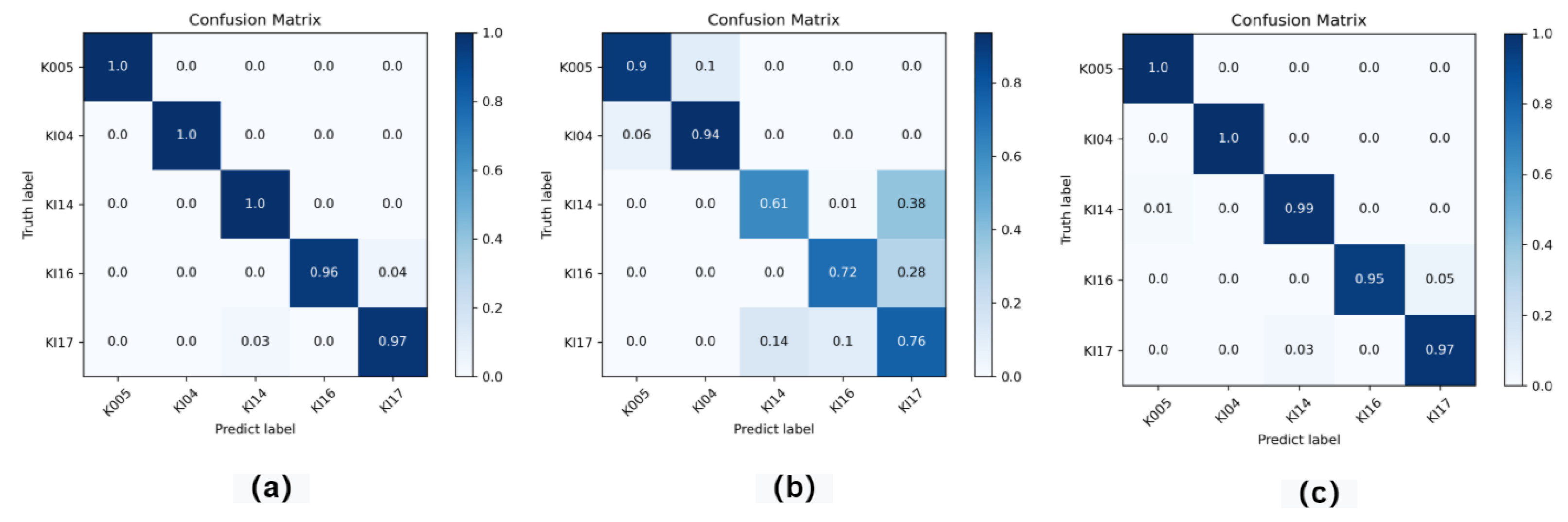
4.4.2. Fault Classification Performance

In order to evaluate the classification performance of the hybrid deep autoencoder network, the accuracy of classifying known types of data in the test set was calculated, as shown in

Table 8. Fault classification accuracy.

	CWRU	Paderborn	MFPT
Ours	100%	98.53%	97.03%
LSTM	79.85%	79.35%	72.89%
SAE	100%	97.98%	96.73%

. It can be clearly seen that the classification performance of our method is not significantly different from that of SAE. The classification results on all three datasets are very good, with almost all samples accurately classified. LSTM has the lowest accuracy; we believe this is due to the poor feature extraction ability of the LSTM model, which makes it unable to make accurate judgments based on the extracted features.

Figure 12, Figure 13 and Figure 14 show the confusion matrices of different methods on classifying known faulty samples in the three datasets. The confusion matrix is a commonly used tool for evaluating the performance of multiclass classification. It presents the correspondence between the model’s predicted results and the true labels in the form of a table. Rows represent the model’s predicted results, while columns represent the true class labels. The values in each cell represent the probability that the model predicts a sample to belong to a certain class. Additionally, we use colors to visually represent the magnitude of the probabilities, where darker colors indicate higher probabilities and lighter colors indicate lower probabilities. Our proposed network and the SAE network can accurately classify each known faulty sample, with classification accuracy exceeding 96%. However, the accuracy of the LSTM autoencoder model is only around 70%. Furthermore, most of the confusion occurs between faults that have the same location but differ in severity. This also indicates that the fault classification ability of the LSTM autoencoder network is inferior to the other two models.

In order to further validate the model’s classification performance on different fault types, we used the t-SNE algorithm [43] to visualize the original data and the data after feature extraction by the network. Through t-SNE visualization, we can observe whether data points form distinct clusters in low-dimensional space. Similar data points will cluster together in the visualization, while different data points will be far apart. Therefore, we can use t-SNE visualization to observe whether features of the same fault type gather together to validate the network’s feature extraction capability. If the network has good feature extraction capability, the features extracted for the same fault type will be very similar and will cluster together in the visualization. Features of different classes will have significant differences and will be far apart. On the other hand, the network’s classification performance mainly depends on whether the features extracted for each class can be separated. Therefore, we used t-SNE in the paper to validate the network’s classification performance.

The visualization results of the original data and the feature data extracted by the two networks on the three datasets are shown in Figure 15, Figure 16 and Figure 17. From the figures, it can be observed that the different fault types in the original data of each dataset are mixed together, making it difficult to distinguish between fault categories. However, the feature data extracted by the hybrid deep autoencoder network on the three datasets can clearly differentiate each fault type after t-SNE dimension reduction, validating the accuracy of the model’s fault classification. There is only a slight overlap between class 3 and class 4 in the Paderborn dataset, resulting in some classification errors. The fault classification ability of LSTM is poor. In the CWRU dataset, it can be clearly seen that there are some samples where it is difficult to distinguish between class 1 and class 3, and some samples are directly misclassified into class 4 and class 5. Some samples are misclassified in the Paderborn dataset, and in the MFPT dataset, a large number of samples are clustered together and cannot be distinguished. We believe that this is due to the severe impact of LSTM’s classification performance under the condition of imbalanced datasets.

4.4.3. Model Complexity Analysis

Figure 18 shows the loss curves of our proposed method on the three datasets. It can be observed that the loss decreases rapidly at the beginning and then gradually converges to the minimum value and stabilizes after 30 epochs.

In order to illustrate the computational complexity of the proposed method, the number of parameters in the model and the average training time required for 40 epochs are listed in

Table 9. Number of parameters and training times for different models.

	Total Params	Training Time (s)
Ours	117,224	203
LSTM	1,084,544	1272
SAE	1,678,629	869

. Our model replaces the fully connected layers of the deep autoencoder with convolutional layers, significantly reducing the number of parameters. As a result, the training is faster compared to other methods, making it advantageous in fault recognition and diagnosis tasks.

5. Conclusions

This paper proposes a novelty detection and fault diagnosis method for bearing fault recognition and diagnosis based on a hybrid deep autoencoder. The method uses one model to accomplish two tasks, detecting new faults and classifying known faults. In order to address the challenge of requiring a large number of training samples in existing deep learning methods, this paper combines the unsupervised training characteristics of autoencoders with the powerful feature extraction ability of convolutional neural networks, adopting a semi-supervised training method that can learn fault features from both labeled and unlabeled samples, reducing the required sample size for training. Compared with existing novelty fault detection methods, the effectiveness of the proposed method is confirmed, with diagnostic accuracy not lower than existing methods, improving the detection accuracy and meeting the requirements of accuracy for both new fault recognition and known fault classification, while speeding up the training speed of the network. However, the hyperparameters of the hybrid deep autoencoder network are mainly set based on conventional experience and continuously adjusted through trial and error to achieve higher diagnostic accuracy. In future work, we need to add some hyperparameter adjustment strategies to help the network find the optimal parameters more quickly. In addition, this method can only detect new faults and cannot differentiate between different new faults, it is unable to represent and distinguish faults in more detail. Therefore, further classification of different types of new faults will be the theme of our future work. We can add some clustering methods to solve this problem, which could be valuable in practical fault diagnosis scenarios.

References

1. Malla, C.; Panigrahi, I. Review of condition monitoring of rolling element bearing using vibration analysis and other techniques. J. Vib. Eng. Technol. 2019, 7, 407–414. [Google Scholar] [CrossRef]
2. Saufi, S.R.; Isham, M.F.; Ahmad, Z.A.; Hasan, M.D.A. Machinery fault diagnosis based on a modified hybrid deep sparse autoencoder using a raw vibration time-series signal. J. Ambient Intell. Humaniz. Comput. 2023, 14, 3827–3838. [Google Scholar] [CrossRef]
3. Asavalertpalakorn, S.; Singhatanadgid, P.; Ardsomang, T. Novelty Detection of a Rolling Bearing using Long Short-Term Memory Autoencoder. In Proceedings of the 2022 37th International Technical Conference on Circuits/Systems, Computers and Communications (ITC-CSCC), Phuket, Thailand, 5–8 July 2022; pp. 1–4. [Google Scholar]
4. Yang, Z.; Gjorgjevikj, D.; Long, J.; Zi, Y.; Zhang, S.; Li, C. Sparse autoencoder-based multi-head deep neural networks for machinery fault diagnostics with detection of novelties. Chin. J. Mech. Eng. 2021, 34, 54. [Google Scholar] [CrossRef]
5. Hoang, D.T.; Kang, H.J. A survey on deep learning based bearing fault diagnosis. Neurocomputing 2019, 335, 327–335. [Google Scholar] [CrossRef]
6. Zhao, R.; Yan, R.; Chen, Z.; Mao, K.; Wang, P.; Gao, R.X. Deep learning and its applications to machine health monitoring. Mech. Syst. Signal Process. 2019, 115, 213–237. [Google Scholar] [CrossRef]
7. Guo, R.; Xu, G.; Yin, Z.; Li, J.; Zhang, F. A Neural Network Method for Bearing Fault Diagnosis. In Proceedings of the 2022 IEEE 8th International Conference on Computer and Communications (ICCC), Virtual, 9–12 December 2022; pp. 116–121. [Google Scholar]
8. Nacer, S.M.; Nadia, B.; Abdelghani, R.; Mohamed, B. A novel method for bearing fault diagnosis based on BiLSTM neural 561 networks. Int. J. Adv. Manuf. Technol. 2023, 125, 1477–1492. [Google Scholar] [CrossRef]
9. Yu, C.; Wang, H. Rolling Bearing Fault Diagnosis Based on BP Neural Network. In Proceedings of the TEPEN 2022: Efficiency and Performance Engineering Network, Baotou, China, 18–21 August 2023; Springer: Berlin/Heidelberg, Germany, 2023; pp. 576–595. [Google Scholar]
10. Guoxin, W.; Ge, W.; Xiuli, L.; Ruilong, D. Bearing Fault Diagnosis Method Based on STFT Image and AlexNet Network. In Proceedings of the TEPEN 2022: Efficiency and Performance Engineering Network, Baotou, China, 18–21 August 2023; Springer: Berlin/Heidelberg, Germany, 2023; pp. 1056–1068. [Google Scholar]
11. Lu, Z.; Qin, Y.; Cheng, X.; Zhang, S.; Zeng, Y. Bearing Fault Diagnosis Method of Bearing Based on LSTM Auto-Encoder. In Proceedings of the 5th International Conference on Electrical Engineering and Information Technologies for Rail Transportation (EITRT) 2021: Rail Transportation System Safety and Maintenance Technologies, Qingdao, China, 21–23 October 2021; pp. 582–591. [Google Scholar]
12. Chi, F.l.; Yang, X.y. Research on simulation of motor bearing fault diagnosis based on auto-encoder. In Proceedings of the Sixth International Conference on Electromechanical Control Technology and Transportation (ICECTT 2021), Chongqing, China, 14–16 May 2021; SPIE: Bellingham, WA, USA, 2022; Volume 12081, pp. 20–28. [Google Scholar]
13. Xu, Y.; Li, C.; Xie, T. Intelligent diagnosis of subway traction motor bearing fault based on improved stacked denoising autoencoder. Shock Vib. 2021, 2021, 6656635. [Google Scholar] [CrossRef]
14. Lu, C.; Wang, Z.Y.; Qin, W.L.; Ma, J. Fault diagnosis of rotary machinery components using a stacked denoising autoencoder-based health state identification. Signal Process. 2017, 130, 377–388. [Google Scholar] [CrossRef]
15. Kiranyaz, S.; Avci, O.; Abdeljaber, O.; Ince, T.; Gabbouj, M.; Inman, D.J. 1D convolutional neural networks and applications: A survey. Mech. Syst. Signal Process. 2021, 151, 107398. [Google Scholar] [CrossRef]
16. Jiao, J.; Zhao, M.; Lin, J.; Liang, K. A comprehensive review on convolutional neural network in machine fault diagnosis. Neurocomputing 2020, 417, 36–63. [Google Scholar] [CrossRef]
17. Xia, M.; Li, T.; Xu, L.; Liu, L.; De Silva, C.W. Fault diagnosis for rotating machinery using multiple sensors and convolutional neural networks. IEEE/ASME Trans. Mechatronics 2017, 23, 101–110. [Google Scholar] [CrossRef]
18. Wen, L.; Li, X.; Gao, L.; Zhang, Y. A new convolutional neural network-based data-driven fault diagnosis method. IEEE Trans. Ind. Electron. 2017, 65, 5990–5998. [Google Scholar] [CrossRef]
19. Zhang, J.; Zhou, Y.; Wang, B.; Wu, Z. Bearing fault diagnosis base on multi-scale 2D-CNN model. In Proceedings of the 2021 3rd International Conference on Machine Learning, Big Data and Business Intelligence (MLBDBI), Taiyuan, China, 3–5 December 2021; pp. 72–75. [Google Scholar]
20. Xu, Y.; Li, Z.; Wang, S.; Li, W.; Sarkodie-Gyan, T.; Feng, S. A hybrid deep-learning model for fault diagnosis of rolling bearings. Measurement 2021, 169, 108502. [Google Scholar] [CrossRef]
21. Guo, Z.; Yang, M.; Huang, X. Bearing fault diagnosis based on speed signal and CNN model. Energy Rep. 2022, 8, 904–913. [Google Scholar] [CrossRef]
22. Xu, T.; Lv, H.; Lin, S.; Tan, H.; Zhang, Q. A fault diagnosis method based on improved parallel convolutional neural network for rolling bearing. Proc. Inst. Mech. Eng. Part J. Aerosp. Eng. 2023, 09544100. [Google Scholar] [CrossRef]
23. Zhang, J.; Yi, S.; Liang, G.; Hongli, G.; Xin, H.; Hongliang, S. A new bearing fault diagnosis method based on modified convolutional neural networks. Chin. J. Aeronaut. 2020, 33, 439–447. [Google Scholar] [CrossRef]
24. Yan, S.; Shao, H.; Xiao, Y.; Liu, B.; Wan, J. Hybrid robust convolutional autoencoder for unsupervised anomaly detection of machine tools under noises. Robot. Comput.-Integr. Manuf. 2023, 79, 102441. [Google Scholar] [CrossRef]
25. Jana, D.; Patil, J.; Herkal, S.; Nagarajaiah, S.; Duenas-Osorio, L. CNN and Convolutional Autoencoder (CAE) based real-time sensor fault detection, localization, and correction. Mech. Syst. Signal Process. 2022, 169, 108723. [Google Scholar] [CrossRef]
26. Zou, L.; Zhuang, K.; Zhou, A.; Hu, J. Bayesian optimization and channel-fusion-based convolutional autoencoder network for fault diagnosis of rotating machinery. Eng. Struct. 2023, 280, 115708. [Google Scholar] [CrossRef]
27. Yu, F.; Liu, J.; Liu, D.; Wang, H. Supervised convolutional autoencoder-based fault-relevant feature learning for fault diagnosis in industrial processes. J. Taiwan Inst. Chem. Eng. 2022, 132, 104200. [Google Scholar] [CrossRef]
28. Zheng, L.; Xu, P.; Bai, J. Power Grid Fault Location Method Based on Pretraining of Convolutional Autoencoder. In Proceedings of the 2021 IEEE International Conference on Computer Science, Artificial Intelligence and Electronic Engineering (CSAIEE), Virtual, 20–22 August 2021; pp. 324–327. [Google Scholar]
29. Song, W.; Lin, J.; Zhou, F.; Li, Z.; Zhao, K.; Zhou, H. Wind turbine bearing fault diagnosis method based on an improved denoising AutoEncoder. Power Syst. Prot. Control 2022, 50, 61–68. [Google Scholar]
30. Wu, X.; Zhang, Y.; Cheng, C.; Peng, Z. A hybrid classification autoencoder for semi-supervised fault diagnosis in rotating machinery. Mech. Syst. Signal Process. 2021, 149, 107327. [Google Scholar] [CrossRef]
31. Zhou, J.; Gao, S.; Li, J.; Xiong, W. Bearing life prediction method based on parallel multichannel recurrent convolutional neural network. Shock Vib. 2021, 2021, 6142975. [Google Scholar] [CrossRef]
32. Niri, M.F.; Bui, T.M.; Dinh, T.Q.; Hosseinzadeh, E.; Yu, T.F.; Marco, J. Remaining energy estimation for lithium-ion batteries via Gaussian mixture and Markov models for future load prediction. J. Energy Storage 2020, 28, 101271. [Google Scholar] [CrossRef]
33. Bui, T.M.N.; Holmes, N.; Dinh, T.Q. Baseline Strategy for Remaining Range Estimation of Electric Motorcycle Applications. In Proceedings of the 2022 25th International Conference on Mechatronics Technology (ICMT), Kaohsiung, Taiwan, 18–21 November 2022; pp. 1–4. [Google Scholar]
34. Del Buono, F.; Calabrese, F.; Baraldi, A.; Paganelli, M.; Regattieri, A. Data-driven predictive maintenance in evolving environments: A comparison between machine learning and deep learning for novelty detection. In Proceedings of the 8th International Conference on Sustainable Design and Manufacturing (KES-SDM 2021), Split, Croatia, 15–17 September 2021; pp. 109–119. [Google Scholar]
35. Wu, H.; Triebe, M.J.; Sutherland, J.W. A transformer-based approach for novel fault detection and fault classification/diagnosis in manufacturing: A rotary system application. J. Manuf. Syst. 2023, 67, 439–452. [Google Scholar] [CrossRef]
36. Jiang, Y.; Sun, H.; Hong, L.; Lin, R.; Yan, W.; Li, Z. Research on Voiceprint Recognition of Electrical Faults With Lower False Alarm Rate. In Proceedings of the 2021 Power System and Green Energy Conference (PSGEC), Shanghai, China, 20–22 August 2021; pp. 599–603. [Google Scholar]
37. Li, Y.; Yang, S.; Wu, J.; Zhongbo, G. Novelty Faults Detection Method Based on SVM Observer and Its Application. J. Vib. Meas. Diagn. 2021, 41, 292–298. [Google Scholar]
38. Górski, J.; Jabłoński, A.; Heesch, M.; Dziendzikowski, M.; Dworakowski, Z. Comparison of novelty detection methods for detection of various rotary machinery faults. Sensors 2021, 21, 3536. [Google Scholar] [CrossRef]
39. Lou, X.; Loparo, K.A. Bearing fault diagnosis based on wavelet transform and fuzzy inference. Mech. Syst. Signal Process. 2004, 18, 1077–1095. [Google Scholar] [CrossRef]
40. Lessmeier, C.; Kimotho, J.K.; Zimmer, D.; Sextro, W. Condition monitoring of bearing damage in electromechanical drive systems by using motor current signals of electric motors: A benchmark data set for data-driven classification. In Proceedings of the PHM Society European Conference, Bilbao, Spain, 5–8 July 2016; Volume 3. [Google Scholar]
41. Bechhoefer, E.; Condition Based Maintenance Fault Database for Testing Diagnostics and Prognostic Algorithms. MFPT Data 2013. Available online: https://www.mfpt.org/fault-data-sets/ (accessed on 23 June 2023).
42. Zhou, Z.H. Machine Learning; Springer Nature: Berlin/Heidelberg, Germany, 2021. [Google Scholar]
43. Van der Maaten, L.; Hinton, G. Visualizing data using t-SNE. J. Mach. Learn. Res. 2008, 9, 2579–2605. [Google Scholar]
Figure 1. Diagram of the hybrid deep autoencoder network module.
Electronics 12 02826 g001
Figure 2. Structures of the encoder and decoder.
Electronics 12 02826 g002
Figure 3. The schematic diagram for selecting the threshold using the boxplot method.
Electronics 12 02826 g003
Figure 4. Softmax structure diagram.
Electronics 12 02826 g004
Figure 5. Flowchart for novelty detection and fault diagnosis in a hybrid deep autoencoder.
Electronics 12 02826 g005
Figure 6. The time-frequency map after wavelet transform.
Electronics 12 02826 g006
Figure 7. Time-frequency plot of the Paderborn dataset.
Electronics 12 02826 g007
Figure 8. Time-frequency plot of MFPT dataset.
Electronics 12 02826 g008
Figure 9. Distribution of reconstruction errors for known and unknown classes on the CWRU dataset.
Electronics 12 02826 g009
Figure 10. Distribution of reconstruction errors for known and unknown classes on the Paderborn dataset.
Electronics 12 02826 g010
Figure 11. Distribution of reconstruction errors for known and unknown classes on the MFPT dataset.
Electronics 12 02826 g011
Figure 12. Confusion matrix on the CWRU dataset. (a) Proposed method. (b) LSTM. (c) SAE.
Electronics 12 02826 g012
Figure 13. Confusion matrix on the Paderborn dataset. (a) Proposed method. (b) LSTM. (c) SAE.
Electronics 12 02826 g013
Figure 14. Confusion matrix on the MFPT dataset. (a) Proposed method. (b) LSTM. (c) SAE.
Electronics 12 02826 g014
Figure 15. Feature visualization on CWRU datasets. (a) Raw data. (b) Proposed method. (c) LSTM.
Electronics 12 02826 g015
Figure 16. Feature visualization on Paderborn datasets. (a) Raw data. (b) Proposed method. (c) LSTM.
Electronics 12 02826 g016
Figure 17. Feature visualization on MFPT datasets. (a) Raw data. (b) Proposed method. (c) LSTM.
Electronics 12 02826 g017
Figure 18. Loss when training on different datasets. (a) CWRU. (b) Paderborn. (c) MFPT.
Electronics 12 02826 g018