Trajectory Tracking Control of Unmanned Surface Vehicles Based on a Fixed-Time Disturbance Observer

Abstract

In ocean environments with unknown complex disturbances, the control accuracy for an unmanned surface vehicle (USV) is severely challenged with an increase in task complexity. As the foundation for executing complex tasks, it is particularly important to control a USV to navigate along a safe trajectory that has been set. In order to effectively handle the trajectory tracking problem, an innovative USV tracking control strategy with high accuracy is proposed by combining the integral sliding-mode and disturbance observer technologies, and these are effectively extended to a scenario with the cooperative trajectory tracking of multiple USVs in this study. Specifically, unknown disturbances are treated as lumped uncertainties, and a novel fixed-time stable-convergence disturbance observer (FT-DO) is proposed to effectively observe and approximate the lumped uncertainties. Then, in order to quickly reach and steadily navigate along the desired trajectory, an effective fixed-time stable-convergence fast integral sliding mode is modified, and on this basis, an accurate trajectory tracking controller (FTFISM-TTC) for a single USV and a cooperative trajectory tracking controller for multiple USVs are meaningfully proposed. Finally, the stability of FT-DO and FTFISM-TTC was rigorously proven by using the Lyapunov approach, and a comprehensive simulation of current advanced tracking control methods was conducted by using Matlab, which proved the reliability of the proposed trajectory tracking control strategy and further eliminated the impact of the initial state on the tracking accuracy.

1. Introduction

With the significant improvement of hardware performance and operability, unmanned surface vehicles (USVs) come to be widely used in military and daily operations instead of humans due to their safety and scalability [1,2]. Especially in high-risk and high-uncertainty missions, USVs can perform tasks endlessly and efficiently on the basis of power support, which has significant effects on important tasks, such as threat monitoring, target reconnaissance, and search and rescue. In the field of intelligent control of USVs, as the foundation for USVs’ performance of other complex tasks, trajectory tracking control has received widespread attention from researchers, and rapid progress has been made in single-USV trajectory tracking [3]. The goal of single-USV trajectory tracking control is to guide and control a USV to arrive at a desired trajectory from any position and to navigate along the desired trajectory with minimal tracking error. It is worth mentioning that a given desired trajectory is a continuous curve composed of a series of waypoints with time constraints in an Earth coordinate system. As the complexity of tasks increases, deficiencies, such as the low efficiency and poor robustness of a single USV, gradually emerge. In order to further improve the efficiency of task completion, multiple USVs can be formed into a designed formation to execute tasks along the set trajectory, which greatly improves the efficiency of highly time-based tasks, such as regional searches.

As an extension of single-USV trajectory tracking control, multiple-USV cooperative trajectory tracking control limits the positioning among USVs by setting the desired navigation trajectory for each USV in advance, thus significantly reducing the task completion time and demonstrating advantages such as high accuracy and robustness. The cooperative trajectory tracking control scenario can be implemented using the formation control framework, and typical formation strategies include leader–follower formation framework, artificial potential field, behavior-based, virtual structure, and graph theory [4,5,6,7,8]. Specifically, a distributed prescribed-time leader–follower formation control scheme for SUV in [4], while meeting the predefined transient performance and overcoming the unknowns and input saturation. In [5], the artificial potential function consisting of formation control term and target tracking term is established for multiple unmanned aerial vehicles, which achieves accurate formation. Considering the problems of unreachable targets and local minimums in artificial potential fields, ref. [6] solves these problems by introducing behavior-based AUG formation control method. However, the disadvantage of this method is that it is difficult to describe the dynamic characteristics of the group, and difficult to control the stability of the formation. In [7], a method of finite-time position and attitude tracking control method combined with artificial potential field and virtual structure is presented, which ensures that the AUVs avoid collisions with each other during the dive, and form and change the formation after reaching the set depth. However, due to the virtual structure method requiring the formation to maintain a rigid structure, its collision avoidance effect is poor. In [8], a distance-based graph rigidity and affine transformation algorithm is used to control a fleet of AUVs to achieve any desired formation shape. Among the above control strategies, the leader–follower formation method is the most commonly referenced because of its simple structure and stable formation. We only need to strictly set the position difference between USVs while ensuring that the leader USV stably navigates along the set trajectory. Inspired by the leader–follower framework proposed in [4], a simple and effective dual layer cooperative trajectory tracking framework is designed to simplify analysis in this paper.

During the process of tracking a desired trajectory, the designed tracking controller should have a fast and stable convergence speed. The common intelligent trajectory tracking control algorithms are as the following: sliding-mode control, backstepping, model predictive control, and fuzzy control. Among the above methods, the backstepping method has good tracking and control performance in ideal conditions, but its performance is poor in situations with unknown external disturbances. In comparison, the sliding-mode control method has the simplest structure, has excellent control performance, and is insensitive to disturbances that may exist [9]. Therefore, as a theoretical basis, sliding-mode control has been widely improved and applied in the field of intelligent control of USVs. Typical improvement methods include integral sliding mode (ISM), terminal sliding mode (TSM), nonsingular terminal sliding mode (NTSM) and adaptive sliding mode scheme [10,11,12,13,14]. The ISM scheme, as a fundamental and effective sliding mode control method, ensures the robustness of the system by determining the appropriate initial position to ensure that the system only has a sliding stage, which is widely used in USV control. In [10], an improved integral sliding mode control attitude controller for AUV with model uncertainties and external disturbances is proposed to improve the ability of attitude tracking. However, due to its insensitivity to disturbances, the tracking performance is poor in non ideal environments. Compared with ISM, the TSM has the characteristics of finite time convergence and stable tracking. In [11], a formation tracking control method for the operation of multiagent systems under disturbances is proposed based on the fast TSM scheme. It is worth mentioning that most TSM schemes cannot eliminate singularity. On the basis of TSM, a time-varying NTSM controller is designed to ensure the global robustness of the USV tracking system with respect to large uncertainties and unknown environmental disturbances in [12]. Although this method effectively eliminates singularity, the convergence time is too dependent on the initial state of the system. In order to further improve the trajectory tracking accuracy in the presence of multiple disturbances, an adaptive sliding-mode unit vector control approach based on monitoring functions is proposed to handle disturbances of unknown bounds in [13,14]. The strategy is able to guarantee a pre-specified transient time, maximum overshoot, and steady-state error for multivariable uncertain plants, which verified its effectiveness in USV trajectory tracking control. It is worth mentioning that [13] provides rigorous theoretical derivation on the proposed adaptive sliding mode strategy, which is lacking in this article and the proposed strategy in this article is more inclined towards application. Compared with other sliding mode methods, the ISM ensures that the system can only have a sliding stage by obtaining an appropriate initial position to ensure robustness. Nevertheless, the ISM has limitations in convergence speed and relies on the initial state of the trajectory tracking. Based on TIM scheme and fixed-time theory, a novel fast integral sliding mode strategy is designed to further optimize convergence speed and stability in this paper.

Due to the limitations of existing trajectory tracking control methods and navigation uncertainties, there is a significant error between the actual navigation path and the expected trajectory. To further improve the trajectory tracking accuracy, combinations of finite-time theory and intelligent control methods can significantly improve the tracking performance of single or multiple USVs [15,16,17]. Nevertheless, finite-time theory cannot eliminate the impact of the initial state of a USV on control performance. To address this drawback, researchers have attempted to apply fixed-time control theory in multi-agent cooperative control to improve the control accuracy while reducing the dependence on the initial states [18,19], which was first proposed and rigorously proven in [20]. Hence, the fixed-time theory was used to optimize the control performance of the sliding-mode control in this study, and then an efficient trajectory tracking controller was designed.

Actual ocean environments have various unknown disturbances, and due to the limitations of sea trials, it is not possible to identify all USV model parameters. Therefore, one must accurately identify the internal and external disturbances present in a tracking system before designing a trajectory tracking controller [21]. The classical disturbance identification methods include active disturbance rejection control, neural network approximation, and Kalman filtering. Nevertheless, these methods have low disturbance processing accuracy and are prone to falling into local minima. On the basis of the above disturbance identification methods, disturbance observer technology has been proposed to identify unknown disturbances in the system and demonstrates excellent identification performance. In [22], a nonlinear disturbance observer is designed to repair the velocity and position information of USVs disturbed by multiple types of noise. In order to perform mixed fault disturbance identification for USV with input saturation constraints, an accurate finite-time convergence observer was designed in [23]. In [24], an improved observer is proposed to observe and handle complex disturbances during USV navigation and control the underactuated USV to accurately track the desired trajectory. To further optimize disturbance identification performance, the idea of extended state observer (ESO) was proposed in [25] and demonstrated excellent performance. For similar disturbance identification, a time-shifted sliding mode observer (SMO) is proposed to solve the problem of fault reconstruction in delayed systems in [26], which utilizes the variation of constants formula to obtain the present time estimate of the unmeasured state, achieving excellent observation results. In [27], a novel time shift approach for actuator fault reconstruction of systems with output time-delay based on a sliding mode observer is proposed to ensure that ideal sliding mode is made possible even in the presence of delay. Although the disturbance observer mentioned above can identify the disturbances present in the system, the identification accuracy of the above disturbance observer technologies will be affected by the initial observation state. Therefore, to further improve the disturbance identification performance and eliminate the impact of initial observation errors, we propose a modified disturbance observer based on fixed time control theory to accurately identify the disturbances existing in cooperative trajectory tracking system.

As mentioned above, in order to ensure that a USV can quickly track a set trajectory and accurately navigate along the desired trajectory with complex internal and external disturbances, a high-performance tracking controller and a high-precision disturbance observer are proposed in this study. Specifically, a modified fixed-time convergence disturbance observer (FT-DO) is proposed to achieve accurate identification of a lumped disturbance term in the tracking control system. Secondly, for a single-USV trajectory tracking control scenario, a reliable fixed-time-convergence fast integral sliding-mode trajectory tracking controller (FTFISM-TTC) is proposed to further improve the trajectory tracking accuracy and convergence speed. Then, a multiple-USV cooperative trajectory tracking controller was designed to demonstrate the scalability of the proposed algorithm. Finally, rigorous theoretical proof and a comprehensive simulation analysis are used to prove that the FTFISM-TTC is superior to the backstepping and TSM in [28]. Compared with the previous works, the main innovations of this paper are as follows.

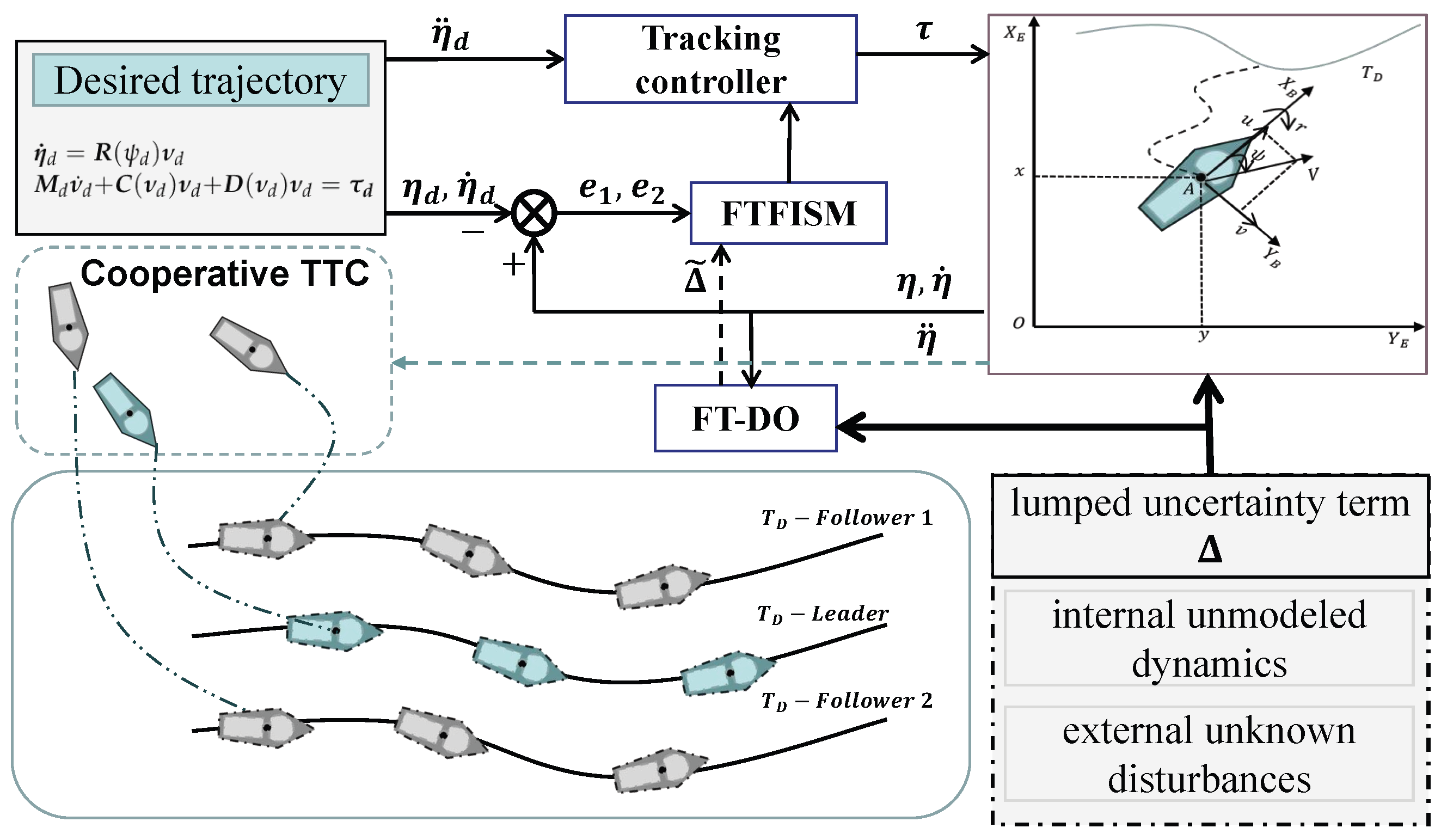
(1) The internal unknown parameter disturbances and external ocean disturbances present in the trajectory tracking control system were considered as a lumped disturbance term. Then, a high-precision fixed-time-convergence disturbance observer (FT-DO) was designed to accurately identify the lumped disturbance term in real time and effectively eliminate the impact of initial errors on the identification accuracy.

(2) After the lumped disturbance term was eliminated, the FTFISM-TTC was proposed to ensure that a USV could quickly navigate to the set trajectory and to ensure stable movement along the current trajectory, while effectively eliminated the dependence of the tracking control accuracy on the initial state. Then, the trajectory tracking control of a single USV was extended to multiple-USV cooperative tracking control within the leader–follower framework, which further verified the scalability and effectiveness of the proposed FTFISM-TTC strategy.

(3) By designing appropriate Lyapunov functions to rigorously analyze the tracking control strategy, the reliability of the designed FT-DO and FTFISM-TTC was proved. At the same time, through comprehensive simulation and comparison experiments in Matlab, the excellent control performance of FT-DO and FTFISM-TTC was further verified.

The structure of the content is as follows: The basic lemmas and mathematical model of USV trajectory tracking are introduced in Section 2. Section 3 describes the design of the FT-DO and FTFISM-TTC, and it provides detailed theoretical derivations and proof of stability. Multiple comprehensive simulation and comparison experiments are described in Section 4. Section 5 provides a detailed summary.

2. Preliminaries and Mathematical Model

To facilitate the subsequent controller design and proof of stability, this section describes the key lemmas needed for disturbance identification and the design of the tracking controller, and it introduces a detailed mathematical USV model.

2.1. Preliminaries

 Lemma 1.

For the following asymptotically stable system [29],

$$\begin{array}{c}\begin{array}{c}\dot{x}\left(\mathrm{t}\right)=f\left(x\left(\mathrm{t}\right)\right),x\left(0\right)=x_0\hfill \\ f\left(0\right)=0,x\in R^n\hfill \end{array}\end{array}$$

(1)

where $x={[x_1,x_2,\dots ,x_n]}^{\mathrm{T}}$ is the state vector of the nonlinear system and $f(·):N\to R^n$ is an upper semicontinuous mapping in an open neighborhood N of the origin such that the set $f\left(x\right)$ is non-empty for any $x\in N$.

The system (1) converges to stability in finite time with a negative degree of homogeneity. If the convergence time set by the system has an upper bound $T_{max}>0$, i.e., $T\left(\epsilon \right)\le T_{max}$ for all $\epsilon \in R^n$, the asymptotically stable system (1) is proven to be fixed-time stable.

 Lemma 2.

For the following system [30],

$$\dot{y}=-{\gamma }_1{y}^{2-p/q}-{\gamma }_2{y}^{p/q},y\left(0\right)=y_0,$$

(2)

if ${\gamma }_1,{\gamma }_2>0$, $p<q$, and both of them represent positive odd integers; then, the scalar system (2) ensures convergence within a fixed time, and the maximum convergence time until stability is calculated as follows:

$$T_{max}\left(y_0\right)=\frac{q\pi }{2\sqrt{{\gamma }_1{\gamma }_2}\left(q-p\right)}$$

(3)

 Lemma 3.

For the following nonlinear system [31],

$$\dot{y}=-\alpha y^A-\beta y^B,y_{\left(0\right)}=y_0$$

(4)

where $\alpha >0,\beta >0$. A is composed of parameters$a_1$ and $a_2$, and it satisfies $A=a_1/a_2$. B is composed of parameters $b_1$ and $b_2$, and it satisfies $B=b_1/b_2$. If the above parameters are positive odd integers that satisfy $a_1>a_2,b_1<b_2<2b_1$, the nonlinear system (4) ensures convergence within a fixed time, and the maximum convergence time until stability is calculated as follows:

$$T_{max}=\frac{a_2}{\alpha (a_1-a_2)}+\frac{b_2}{\beta (b_2-b_1)}$$

(5)

2.2. Mathematical Model

Due to the limitations of ocean experiments, the model parameters of USVs could not be fully obtained. At the same time, stability is severely affected by unknown disturbances, such as wind, waves, and currents, when a USV performs tasks in actual ocean environments. Therefore, under the premise of reflecting the trajectory tracking characteristics of USVs as much as possible, a three-DOF mathematical USV model containing a lumped disturbance term was designed based on the Cybership II USV model shown in Figure 1a, which included the yaw angular speed r, sway speed v, and surge speed u. It is worth mentioning that the scalar-variable description of the roto-translational motion of a rigid object looks a bit obsolete, and the models proposed in [32,33] based on lie group and manifold theory are more advanced. However, the USV mathematical model used in this article can clearly reflect the motion mechanism of the USV and simplify the controller design process.

Figure 1b shows the three-DOF mathematical USV model. The kinetic and dynamic models of a single USV can be expressed as follows:

$$\begin{array}{c}\left\{\begin{array}{c}\dot{\mathit{\eta }}=\mathit{R}\left(\psi \right)\mathit{\nu }\hfill \\ \mathit{M}\dot{\mathit{\nu }}+\mathit{C}\left(\mathit{\nu }\right)\mathit{\nu }+\mathit{D}\left(\mathit{\nu }\right)\mathit{\nu }=\mathit{\delta }+\mathit{\tau }\hfill \end{array}\right.\end{array}$$

(6)

where $\mathit{\eta }={\left[x,y,\psi \right]}^{\mathrm{T}}$ represents the three different dimensional vectors contained in the kinematic model, $\mathit{\nu }={[u,v,r]}^{\mathrm{T}}$ represents the three different dimensional vectors contained in the dynamic model, and $\mathit{\tau }={[{\tau }_{\mathrm{i}1},0,{\tau }_{\mathrm{i}3}]}^{\mathrm{T}}$ represents the control input of the USV in the forward direction and in steering. The unknown external disturbance term $\mathit{\delta }=\mathit{M}{\mathit{R}}^{\mathrm{T}}\left(\psi \right)\mathit{d}\left(t\right)$ is caused by wind, waves, and currents, and $\mathit{R}\left(\psi \right)$ represents the rotation matrix between the Earth coordinate system and the relative motion coordinate system, which satisfies the following characteristics:

$$\begin{array}{c}\begin{array}{c}\dot{\mathit{R}}\left(\psi \right)=\mathit{R}\left(\psi \right)\mathit{S}\left(r\right)\hfill \\ {\mathit{R}}^{\mathrm{T}}\left(\psi \right)\mathit{S}\left(r\right)\mathit{R}\left(\psi \right)=\mathit{R}\left(\psi \right)\mathit{S}\left(r\right){\mathit{R}}^{\mathrm{T}}\left(\psi \right)=\mathit{S}\left(r\right)\hfill \\ ∥\mathit{R}\left(\psi \right)∥=1,{\mathit{R}}^{\mathrm{T}}\left(\psi \right)\mathit{R}\left(\psi \right)=\mathrm{I},\forall \psi \in [0,2\pi ]\hfill \end{array}\end{array}$$

(7)

where

$$\begin{array}{c}\mathit{R}\left(\psi \right)=\left[\begin{array}{ccc}cos\psi & -sin\psi & 0\\ sin\psi & cos\psi & 0\\ 0& 0& 1\end{array}\right]\end{array}$$

(8)

$$\begin{array}{c}\mathit{S}\left(r\right)=\left[\begin{array}{ccc}0& -r& 0\\ r& 0& 0\\ 0& 0& 0\end{array}\right]\end{array}$$

(9)

The matrix $\mathit{M}={\mathit{M}}^{\mathrm{T}}>0$ represents the inertia matrix during the USV’s motion, and $\mathit{C}\left(\nu \right)=-\mathit{C}{\left(\nu \right)}^{\mathrm{T}}$ and $\mathit{D}\left(\nu \right)$ represent the ocean testing parameter matrices, which include unmodeled dynamics in the USV model. The structure of the above matrices is represented as follows:

$$\begin{array}{c}\mathit{C}\left(\mathit{\nu }\right)=\left[\begin{array}{ccc}0& 0& c_{13}\left(\nu \right)\\ 0& 0& c_{23}\left(\nu \right)\\ -c_{13}\left(\nu \right)& -c_{23}\left(\nu \right)& 0\end{array}\right]\end{array}$$

(10)

$$\begin{array}{c}\mathit{D}\left(\mathit{\nu }\right)=\left[\begin{array}{ccc}{d}_{11}\left(\nu \right)& 0& 0\\ 0& d_{22}\left(\nu \right)& d_{23}\left(\nu \right)\\ 0& -d_{32}\left(\nu \right)& d_{33}\left(\nu \right)\end{array}\right]\end{array}$$

(11)

$$\begin{array}{c}\mathit{M}=\left[\begin{array}{ccc}{m}_{11}& 0& 0\\ 0& m_{22}& m_{23}\\ 0& m_{32}& m_{33}\end{array}\right]\end{array}$$

(12)

The simplification of the mathematical USV model (6) by using the Lagrange equation is as follows:

$$\begin{array}{c}\tilde{\mathit{M}}\left(\mathit{\eta }\right)\ddot{\mathit{\eta }}+\tilde{\mathit{C}}(\mathit{\eta },\dot{\mathit{\eta }})\dot{\mathit{\eta }}+\tilde{\mathit{D}}(\mathit{\eta },\dot{\mathit{\eta }})\dot{\mathit{\eta }}=\mathit{R}\left(\mathit{\eta }\right)\mathit{\tau }+\mathit{\delta }\left(t\right)\end{array}$$

(13)

The transformed inertia matrix $\tilde{\mathit{M}}$, skew-symmetric matrix $\tilde{\mathit{C}}$, and damping matrix $\tilde{\mathit{D}}$ are as follows:

$$\begin{array}{c}\begin{array}{c}\tilde{\mathit{M}}\left(\mathit{\eta }\right)=\mathit{R}\left(\mathit{\eta }\right)\mathit{M}{\mathit{R}}^{\mathrm{T}}\left(\mathit{\eta }\right)\hfill \\ \tilde{\mathit{C}}(\mathit{\eta },\dot{\mathit{\eta }})=\mathit{R}\left(\mathit{\eta }\right)(\mathit{C}-\mathit{MS}){\mathit{R}}^{\mathrm{T}}\left(\mathit{\eta }\right)\hfill \\ \tilde{\mathit{D}}(\mathit{\eta },\dot{\mathit{\eta }})=\mathit{R}\left(\mathit{\eta }\right)\mathit{D}{\mathit{R}}^{\mathrm{T}}\left(\mathit{\eta }\right)\hfill \\ \mathit{M}\left(\mathit{\eta }\right)={\mathit{M}}^{\mathrm{T}}\left(\mathit{\eta }\right)>0\hfill \\ \dot{\mathit{M}}\left(\mathit{\eta }\right)-2\mathit{C}(\mathit{\eta },\dot{\mathit{\eta }})=-{[\dot{\mathit{M}}\left(\mathit{\eta }\right)-2\mathit{C}(\mathit{\eta },\dot{\mathit{\eta }})]}^{\mathrm{T}}\hfill \end{array}\end{array}$$

(14)

Let ${\mathit{x}}_1=\mathit{\eta }$, ${\mathit{x}}_2=\dot{\mathit{\eta }}$, and the internal unknown parameters and external complex disturbances are treated as a lumped disturbance term $\mathbf{\Delta }$, which satisfies the condition of being continuously differentiable and bounded: $\mathbf{\Delta }={\tilde{\mathit{M}}}^{-1}\left[\mathit{\delta }\left(t\right)-\tilde{\mathit{C}}({\mathit{x}}_1,{\mathit{x}}_2){\mathit{x}}_2-\tilde{\mathit{D}}({\mathit{x}}_1,{\mathit{x}}_2){\mathit{x}}_2\right]$. Then, we simplify (13) as follows:

$$\begin{array}{c}\left\{\begin{array}{c}{\dot{\mathit{x}}}_1={\mathit{x}}_2\hfill \\ {\dot{\mathit{x}}}_2={\tilde{\mathit{M}}}^{-1}\left({\mathit{x}}_1\right)\mathit{R}\left({\mathit{x}}_1\right)\mathit{\tau }+\mathbf{\Delta }\hfill \end{array}\right.\end{array}$$

(15)

The detailed parameter explanations for $\mathit{M},\mathit{C},\mathit{D}$ are shown in

Table 1. Detailed matrix parameters for $\mathit{M},\mathit{C},\mathit{D}$.

Parameter	Formula	Parameter	Formula
$m_{11}$	$m-X_{\dot{u}}$	$m_{22}$	$m-Y_{\dot{v}}$
$m_{23}$	$m{x}_g-Y_{\dot{r}}$	$m_{32}$	$m{x}_g-N_{\dot{v}}$
$m_{33}$	$I_z-N_{\dot{r}}$	$c_{13}\left(\nu \right)$	$m_{11}-m_{23}r$
$c_{23}\left(\nu \right)$	$m_{11}u$	$d_{11}\left(\nu \right)$	$-X_u-X_{\left|u\right|u}\left|u\right|-X_{uuu}{u}^2$
$d_{22}\left(\nu \right)$	$-Y_v-Y_{\left|vs.\right|v}\left|vs.\right|$	$d_{23}\left(\nu \right)$	$-Y_r-Y_{\left|vs.\right|r}\left|vs.\right|-Y_{\left|r\right|r}\left|r\right|$
$d_{32}\left(\nu \right)$	$$\begin{gathered} -N_v-N_{\left|vs.\right|v}\left|vs.\right|- \\ {\mathit{\hspace{1em}\hspace{1em}\hspace{1em} N}}_{\left|r\right|v}\left|r\right| \end{gathered}$$	$d_{33}\left(\nu \right)$	$-N_r-N_{\left|vs.\right|r}\left|vs.\right|-N_{\left|r\right|r}\left|r\right|$

. The terms m and $I_z$ represent the mass and the moment of inertia of the USV, $N_{\dot{v}}=Y_{\dot{r}}$, and $X_{*},Y_{*},Z_{*}$ represent the sea trial parameters for hydrodynamics.

The desired trajectory tracking model is represented as follows:

$$\begin{array}{c}\begin{array}{c}{\dot{\mathit{\eta }}}_d=\mathit{R}\left({\psi }_d\right){\mathit{\nu }}_d\hfill \\ {\mathit{M}}_d{\dot{\mathit{\nu }}}_d+\mathit{C}\left({\mathit{\nu }}_d\right){\mathit{\nu }}_d+\mathit{D}\left({\mathit{\nu }}_d\right){\mathit{\nu }}_d={\mathit{\tau }}_{\mathit{d}}\hfill \end{array}\end{array}$$

(16)

where ${\mathit{\tau }}_d={[{\tau }_{d1},0,{\tau }_{d3}]}^{\mathrm{T}}$ represents the ideal speed and steering input for the USV tracking the desired trajectory, and ${\mathit{\eta }}_d={[{\mathrm{x}}_d,{\mathrm{y}}_d,{\psi }_d]}^{\mathrm{T}}$ and ${\mathit{\nu }}_d={[{\mathrm{u}}_d,{\mathrm{v}}_d,r_d]}^{\mathrm{T}}$ represent the ideal states of the USV when sailing along the desired trajectory without disturbances.

3. Disturbance Identification and Trajectory Tracking Controller Design

In the disturbance identification section, a novel fixed-time convergence disturbance observer is designed to ensure the accurate estimation of disturbances. Then, an accurate trajectory tracking control strategy is proposed based on a modified sliding-mode control and the fixed-time theory to ensure that a single USV can quickly reach a desired tracking trajectory and stabilize its navigation. Finally, the single-USV trajectory tracking control is expanded to multiple USVs, and a cooperative tracking controller is proposed by using the leader–follower framework. The overall cooperative trajectory tracking framework is shown in Figure 2.

3.1. Design and Analysis of the Stability of the FT-DO

As mentioned earlier, the internal unknown parameters and external complex disturbances in trajectory tracking are regarded as a lumped disturbance term $\mathbf{\Delta }$, which directly causes errors between the USV and the desired position. Therefore, to simplify the design of the disturbance observer, an auxiliary variable is introduced as follows:

$$\begin{array}{c}\dot{\mathbf{\Phi }}={\tilde{\mathit{M}}}^{-1}\left({\mathit{x}}_{\mathit{1}}\right)\mathit{R}\left({\mathit{x}}_{\mathit{1}}\right)\mathit{\tau }+\lambda {\mathbf{\Phi }}_e\end{array}$$

(17)

where ${\mathbf{\Phi }}_e={\mathit{x}}_{\mathit{2}}-\mathbf{\Phi }$, and $\lambda$ is a normal number.

By combining the mathematical model of USV, the following fixed-time disturbance observer (FT-DO) is proposed:

$$\begin{array}{c}\hat{\mathbf{\Delta }}=\lambda {\hat{\mathbf{\Phi }}}_e+{\dot{\mathbf{\Phi }}}_{\mathit{e}}\end{array}$$

(18)

where $\hat{\mathbf{\Delta }}={\left[{\hat{\Delta }}_{i,1},{\hat{\Delta }}_{i,2},{\hat{\Delta }}_{i,3}\right]}^{\mathrm{T}}$ represents the disturbance observation values of three different dimensions of $\mathbf{\Delta }$. ${\widehat{\mathbf{\Phi }}}_{\mathit{e}}$ is the state estimate of ${\mathbf{\Phi }}_{\mathit{e}}$, and the derivative is given by:

$$\begin{array}{c}{\dot{\widehat{\mathbf{\Phi }}}}_e={\dot{\mathbf{\Phi }}}_{\mathit{e}}+{\alpha }_{i,1}sign{\left({\tilde{\mathbf{\Phi }}}_e\right)}^{{\beta }_{i,1}}+{\alpha }_{i,2}sign{\left({\tilde{\mathbf{\Phi }}}_e\right)}^{{\beta }_{i,2}}+{\alpha }_{i,3}{\tilde{\mathbf{\Phi }}}_e\end{array}$$

(19)

where ${\tilde{\mathbf{\Phi }}}_e={\mathbf{\Phi }}_{\mathit{e}}-{\widehat{\mathbf{\Phi }}}_e$ represents the estimation error of the FT-DO, and ${\alpha }_{i,1},{\alpha }_{i,2},{\alpha }_{i,3}>0$ and ${\beta }_{i,2}>1>{\beta }_{i,1}>0$ represent disturbance observer’s gain.

 Theorem 1.

Let $\tilde{\mathbf{\Delta }}$ be the disturbance observation error between the disturbance observation value and the lumped disturbance term Δ. The designed FT-DO can achieve fixed-time stability and ensure that the observation error converges to zero within a fixed time, i.e., when $t\ge T$, $\tilde{\mathbf{\Delta }}\left(t\right)=0$. Then, the maximum convergence time of the designed FT-DO is obtained as follows:

$$\begin{array}{c}T\le T_{MAX}:=\frac{1}{2^{\frac{1+{\beta }_{i,1}}{2}}{\alpha }_{i,1}(1-{\beta }_{i,1})}+\frac{1}{2^{\frac{1+{\beta }_{i,2}}{2}}{\alpha }_{i,2}({\beta }_{i,2}-1)}\end{array}$$

(20)

 Proof of Theorem 1.

From the above formula, the derivative of the estimation error ${\tilde{\mathbf{\Phi }}}_e$ is calculated as follows:

$$\begin{array}{c}{\dot{\tilde{\mathbf{\Phi }}}}_e={\dot{\mathbf{\Phi }}}_e-{\dot{\widehat{\mathbf{\Phi }}}}_e\hfill \\ ={\dot{\mathbf{\Phi }}}_e-{\dot{\mathbf{\Phi }}}_e-{\alpha }_{i,1}sign{\left({\tilde{\mathbf{\Phi }}}_e\right)}^{{\beta }_{i,1}}-{\alpha }_{i,2}sign{\left({\tilde{\mathbf{\Phi }}}_e\right)}^{{\beta }_{i,2}}-{\alpha }_{i,3}{\tilde{\mathbf{\Phi }}}_e\hfill \\ =-{\alpha }_{i,1}sign{\left({\tilde{\mathbf{\Phi }}}_e\right)}^{{\beta }_{i,1}}-{\alpha }_{i,2}sign{\left({\tilde{\mathbf{\Phi }}}_e\right)}^{{\beta }_{i,2}}-{\alpha }_{i,3}{\tilde{\mathbf{\Phi }}}_e\hfill \end{array}$$

(21)

The following Lyapunov function is selected:

$$\begin{array}{c}{V}_{\mathbf{\Phi }}=\frac{1}{2}{{\tilde{\mathbf{\Phi }}}_e}^T{\tilde{\mathbf{\Phi }}}_e\end{array}$$

(22)

The derivative of Equation (22) is taken as follows:

$$\begin{array}{c}\begin{array}{c}{\dot{V}}_{\mathbf{\Phi }}={{\tilde{\mathbf{\Phi }}}_e}^T{\dot{\tilde{\mathbf{\Phi }}}}_e\hfill \\ ={{\tilde{\mathbf{\Phi }}}_e}^T[-{\alpha }_{i,1}sign{\left({\tilde{\mathbf{\Phi }}}_e\right)}^{{\beta }_{i,1}}-{\alpha }_{i,2}sign{\left({\tilde{\mathbf{\Phi }}}_e\right)}^{{\beta }_{i,2}}-{\alpha }_{i,3}{\tilde{\mathbf{\Phi }}}_e]\hfill \\ \le -{\alpha }_{i,1}{{\tilde{\mathbf{\Phi }}}_e}^{T}sign{\left({\tilde{\Phi }}_e\right)}^{{\beta }_{i,1}}-{\alpha }_{i,2}{{\tilde{\mathbf{\Phi }}}_e}^{T}sign{\left({\tilde{\mathbf{\Phi }}}_e\right)}^{{\beta }_{i,2}}\hfill \\ \le -{\alpha }_{i,1}·{\left[2·\frac{1}{2}{∥{\tilde{\mathbf{\Phi }}}_e∥}^2\right]}^{\frac{1+{\beta }_{i,1}}{2}}-{\alpha }_{i,2}{\left[2·\frac{1}{2}{∥{\tilde{\mathbf{\Phi }}}_e∥}^2\right]}^{\frac{1+{\beta }_{i,2}}{2}}\hfill \\ \le -2^{\frac{1+{\beta }_{i,1}}{2}}{\alpha }_{i,1}{V_{\mathbf{\Phi }}}^{\frac{1+{\beta }_{i,1}}{2}}-2^{\frac{1+{\beta }_{i,2}}{2}}{\alpha }_{i,2}{V_{\mathbf{\Phi }}}^{\frac{1+{\beta }_{i,2}}{2}}\hfill \end{array}\end{array}$$

(23)

According to Lemma 3, the estimation error ${\tilde{\mathbf{\Phi }}}_e$ of the FT-DO achieves fixed-time stability, and the maximum convergence time of the designed FT-DO is obtained as follows:

$$\begin{array}{c}T\le T_{MAX}:=\frac{1}{2^{\frac{1+{\beta }_{i,1}}{2}}{\alpha }_{i,1}(1-{\beta }_{i,1})}+\frac{1}{2^{\frac{1+{\beta }_{i,2}}{2}}{\alpha }_{i,2}({\beta }_{i,2}-1)}\end{array}$$

(24)

By combining (15) and (18), the disturbance observation error between the disturbance observation value and the lumped disturbance term $\mathbf{\Delta }$ can be calculated as follows:

$$\begin{array}{c}\begin{array}{c}\tilde{\mathbf{\Delta }}=\mathbf{\Delta }-\widehat{\mathbf{\Delta }}\hfill \\ ={\dot{\mathit{x}}}_2-{\tilde{\mathit{M}}}^{-1}\left({\mathit{x}}_1\right)\mathit{R}\left({\mathit{x}}_1\right)\mathit{\tau }-\lambda {\widehat{\mathbf{\Phi }}}_e-{\dot{\mathbf{\Phi }}}_e\hfill \\ ={\dot{\mathit{x}}}_2-{\tilde{\mathit{M}}}^{-1}\left({\mathit{x}}_1\right)\mathit{R}\left({\mathit{x}}_1\right)\mathit{\tau }-\lambda {\widehat{\mathbf{\Phi }}}_e-{\dot{\mathit{x}}}_2+\dot{\mathbf{\Phi }}\hfill \\ =-{\tilde{\mathit{M}}}^{-1}\left({\mathit{x}}_1\right)\mathit{R}\left({\mathit{x}}_1\right)\mathit{\tau }-\lambda {\widehat{\mathbf{\Phi }}}_e+{\tilde{\mathit{M}}}^{-1}\left({\mathit{x}}_1\right)\mathit{R}\left({\mathit{x}}_1\right)\mathit{\tau }+\lambda {\mathbf{\Phi }}_e\hfill \\ =\lambda \left({\mathbf{\Phi }}_{\mathit{e}}-{\widehat{\mathbf{\Phi }}}_e\right)\hfill \\ =\lambda {\tilde{\mathbf{\Phi }}}_e\hfill \end{array}\end{array}$$

(25)

To summarize, when $t\ge T$, $\tilde{\mathbf{\Delta }}\left(t\right)=0$, the disturbance observation error converges within a fixed time.

The proof of Theorem 1 and the fixed-time stability of the FT-DO is complete. □

3.2. Design and Analysis of the Stability of the FTFISM-TTC

After disturbance identification, in order to ensure that the USV can quickly and accurately track the desired trajectory, an efficient tracking trajectory controller that effectively eliminates the impact of the initial tracking error on tracking accuracy must be designed.

The real-time tracking error of the USV is defined as follows:

$$\begin{array}{c}\left\{\begin{array}{c}{\mathit{x}}_e^1={\mathit{x}}_1-{\mathit{\eta }}_d\hfill \\ {\mathit{x}}_e^2={\mathit{x}}_2-{\dot{\mathit{\eta }}}_d\hfill \end{array}\right.\end{array}$$

(26)

The derivation of (26) is as follows:

$$\begin{array}{c}\left\{\begin{array}{c}{\dot{\mathit{x}}}_e^1={\mathit{x}}_e^2\hfill \\ {\dot{\mathit{x}}}_e^2={\tilde{\mathit{M}}}^{-1}\left({\mathit{x}}_1\right)\mathit{R}\left({\mathit{x}}_1\right)\mathit{\tau }+\mathbf{\Delta }-{\ddot{\mathit{\eta }}}_d\hfill \end{array}\right.\end{array}$$

(27)

Based on the characteristics of not relying on the initial state and the high robustness of fixed-time control and the integral sliding mode, a novel fixed-time-convergence fast integral sliding mode (FTFISM) is proposed as follows:

$$\begin{array}{c}\begin{array}{c}\mathit{S}\left(t\right)={\mathit{x}}_e^2\left(t\right)+k_s{\int }_0^t(\mu \left({\mathit{x}}_e^1\left(\sigma \right)\right)+\mu \left({\mathit{x}}_e^2\left(\sigma \right)\right))d\sigma \\ \mu \left({\mathit{x}}_e^1\left(\sigma \right)\right)=a_{1}si{g}^{{\vartheta }_1}\left({\mathit{x}}_e^1\left(\sigma \right)\right)+a_{2}sig\left({\mathit{x}}_e^1\left(\sigma \right)\right)+a_{3}si{g}^{{\vartheta }_2}\left({\mathit{x}}_e^1\left(\sigma \right)\right)\\ \mu \left({\mathit{x}}_e^2\left(\sigma \right)\right)=b_{1}si{g}^{{\vartheta }_3}\left({\mathit{x}}_e^2\left(\sigma \right)\right)+b_{2}sig\left({\mathit{x}}_e^2\left(\sigma \right)\right)+b_{3}si{g}^{{\vartheta }_4}\left({\mathit{x}}_e^2\left(\sigma \right)\right)\end{array}\end{array}$$

(28)

where $k_s$ represents integral sliding-mode gain. $a_i,b_i>0.(i=1,2,3)$, $1>{\vartheta }_1,{\vartheta }_3>0$, $2>{\vartheta }_2,{\vartheta }_4>1$.

The derivation of (28) is as follows:

$$\begin{array}{c}\begin{array}{c}\dot{\mathit{S}}\left(t\right)={\dot{\mathit{x}}}_e^2\left(t\right)+k_s(\mu \left({\mathit{x}}_e^1\left(t\right)\right)+\mu \left({\mathit{x}}_e^2\left(t\right)\right))\hfill \\ ={\tilde{\mathit{M}}}^{-1}\left({\mathit{x}}_1\right)\mathit{R}\left({\mathit{x}}_1\right)\mathit{\tau }+\mathbf{\Delta }-{\ddot{\mathit{\eta }}}_d+k_s(\mu \left({\mathit{x}}_e^1\left(t\right)\right)+\mu \left({\mathit{x}}_e^2\left(t\right)\right))\hfill \end{array}\end{array}$$

(29)

By combining (29) and Lemma 2, the fixed-time-convergence fast integral sliding-mode trajectory tracking controller (FTFISM-TTC) is proposed as follows:

$$\begin{array}{c}\mathit{\tau }=-\tilde{\mathit{M}}\mathit{R}(\widehat{\mathbf{\Delta }}-{\ddot{\mathit{\eta }}}_d+k_s(\mu \left({\mathit{x}}_e^1\left(t\right)\right)+\mu \left({\mathit{x}}_e^2\left(t\right)\right))+l_0\mathit{S}+l_1{\mathit{S}}^{2-\frac{m}{n}}+l_2{\mathit{S}}^{\frac{m}{n}})\end{array}$$

(30)

where $l_0,l_1,l_2>0$. $m<n$, and both of them are positive odd integers.

 Theorem 2.

After disturbance identification, the proposed FTFISM-TTC can achieve fixed-time stable convergence and ensure that the USV can quickly and accurately track a trajectory in both the position and velocity dimensions.

 Proof of Theorem 2.

Firstly, in order to demonstrate that the cooperative trajectory tracking control errors ${\mathbf{x}}_e^1$, and ${\mathbf{x}}_e^2$ can quickly reach the surface of the FTFISM and achieve fixed-time convergence, we select the following Lyapunov function:

$${\mathit{V}}_s=\frac{1}{2}{\mathit{S}}^{\mathrm{T}}\mathit{S}$$

(31)

By combining (28) and (29), the derivative of (31) is taken as follows:

$$\begin{array}{c}\begin{array}{c}{\dot{\mathit{V}}}_s={\mathit{S}}^{\mathrm{T}}\dot{\mathit{S}}\hfill \\ ={\mathit{S}}^{\mathrm{T}}[{\dot{\mathit{x}}}_e^2\left(t\right)+k_s(\mu \left({\mathit{x}}_e^1\left(t\right)\right)+\mu \left({\mathit{x}}_e^2\left(t\right)\right))]\hfill \\ ={\mathit{S}}^{\mathrm{T}}[{\tilde{\mathit{M}}}^{-1}\left({\mathit{x}}_1\right)\mathit{R}\left({\mathit{x}}_1\right)\mathit{\tau }+\mathbf{\Delta }-{\ddot{\mathit{\eta }}}_d+k_s(\mu \left({\mathit{x}}_e^1\left(t\right)\right)+\mu \left({\mathit{x}}_e^2\left(t\right)\right))]\hfill \end{array}\end{array}$$

(32)

Combining this with (30), the above formula is simplified as follows:

$$\begin{array}{c}\begin{array}{c}{\dot{\mathit{V}}}_s={\mathit{S}}^{\mathrm{T}}\{{\tilde{\mathit{M}}}^{-1}\left({\mathit{x}}_1\right)\mathit{R}\left({\mathit{x}}_1\right)[-\tilde{\mathit{M}}\left({\mathit{x}}_1\right)\mathit{R}\left({\mathit{x}}_1\right)(\widehat{\mathbf{\Delta }}-{\ddot{\mathit{\eta }}}_d+k_s(\mu \left({\mathit{x}}_e^1\left(t\right)\right)+\mu \left({\mathit{x}}_e^2\left(t\right)\right))\hfill \\ +l_0\mathit{S}+l_1{\mathit{S}}^{2-\frac{m}{n}}+l_2{\mathit{S}}^{\frac{m}{n}})+\mathbf{\Delta }-{\ddot{\mathit{\eta }}}_d+k_s(\mu \left({\mathit{x}}_e^1\left(t\right)\right)+\mu \left({\mathit{x}}_e^2\left(t\right)\right)]\}\hfill \\ =-{\mathit{S}}^{\mathrm{T}}[l_0\mathit{S}+l_1{\mathit{S}}^{2-\frac{m}{n}}+l_2{\mathit{S}}^{\frac{m}{n}}+(\widehat{\mathbf{\Delta }}-\mathbf{\Delta })]\hfill \end{array}\end{array}$$

(33)

In the previous section, the lumped disturbance term $\mathbf{\Delta }$ was accurately identified and compensated by the designed FT-DO in the USV trajectory tracking control, i.e., when $t\ge T$, $\tilde{\mathbf{\Delta }}=\mathbf{\Delta }-\widehat{\mathbf{\Delta }}=0$. Then, the above formula can be simplified as follows:

$$\begin{array}{c}\begin{array}{c}{\dot{\mathit{V}}}_s=-{\mathit{S}}^{\mathrm{T}}[l_0\mathit{S}+l_1{\mathit{S}}^{2-\frac{m}{n}}+l_2{\mathit{S}}^{\frac{m}{n}}+(\widehat{\mathbf{\Delta }}-\mathbf{\Delta })]\hfill \\ =-{\mathit{S}}^{\mathrm{T}}(l_0\mathit{S}+l_1{\mathit{S}}^{2-\frac{m}{n}}+l_2{\mathit{S}}^{\frac{m}{n}})\hfill \\ =-l_0{\mathit{S}}^{\mathrm{T}}\mathit{S}-l_1{\mathit{S}}^{\mathrm{T}}{\mathit{S}}^{2-\frac{m}{n}}-l_2{\mathit{S}}^{\mathrm{T}}{\mathit{S}}^{\frac{m}{n}}\hfill \\ \le -l_1\times 2^{\frac{3n-m}{2n}}{\left(\frac{1}{2}{\mathit{S}}^2\right)}^{\frac{3n-m}{2n}}-l_2\times 2^{\frac{n+m}{2n}}{\left(\frac{1}{2}{\mathit{S}}^2\right)}^{\frac{n+m}{2n}}\hfill \\ \le -2^{\frac{3n-m}{2n}}{l}_1{{\mathit{V}}_s}^{2-\frac{n+m}{2n}}-2^{\frac{n+m}{2n}}{l}_2{{\mathit{V}}_s}^{\frac{n+m}{2n}}\hfill \end{array}\end{array}$$

(34)

Let $A_1=2^{\frac{3n-m}{2n}}{l}_1$, $A_2=2^{\frac{n+m}{2n}}{l}_2$, $B_1=n+m$, $B_2=2n$. The above formula can be simplified as follows:

$$\begin{array}{c}{\dot{\mathit{V}}}_s\le -A_1{{\mathit{V}}_s}^{2-\frac{B_1}{B_2}}-A_2{{\mathit{V}}_s}^{\frac{B_1}{B_2}}\end{array}$$

(35)

According to Lemma 2, the maximum convergence time during the reaching phase is calculated as follows:

$$\begin{array}{c}{T}_S=\frac{B_2\pi }{2\sqrt{A_1{A}_2}(B_2-B_1)}\end{array}$$

(36)

After arriving at the sliding surface, $\mathit{S}=0,\dot{\mathit{S}}=0$. Then, we can obtain

$$\begin{array}{c}\begin{array}{c}{\dot{\mathit{x}}}_e^2\left(t\right)=-k_s(\mu \left({\mathit{x}}_e^1\left(t\right)\right)+\mu \left({\mathit{x}}_e^2\left(t\right)\right))\hfill \\ =-a_1{k}_{s}si{g}^{{\vartheta }_1}\left({\mathit{x}}_e^1\left(\sigma \right)\right)-a_2{k}_{s}sig\left({\mathit{x}}_e^1\left(\sigma \right)\right)-a_3{k}_{s}si{g}^{{\vartheta }_2}\left({\mathit{x}}_e^1\left(\sigma \right)\right)\hfill \\ -b_1{k}_{s}si{g}^{{\vartheta }_3}\left({\mathit{x}}_e^2\left(\sigma \right)\right)-b_2{k}_{s}sig\left({\mathit{x}}_e^2\left(\sigma \right)\right)-b_3{k}_{s}si{g}^{{\vartheta }_4}\left({\mathit{x}}_e^2\left(\sigma \right)\right)\hfill \end{array}\end{array}$$

(37)

According to Lemma 3, the tracking errors ${\mathit{x}}_e^1\left(t\right),{\mathit{x}}_e^2\left(t\right)$ will achieve fixed-time stability during the sliding stage and ultimately converge to zero.

In summary, the designed FTFISM-TTC can ensure fixed-time stability, and the trajectory tracking error quickly converges to zero to achieve precise tracking performance.

The proof of Theorem 2 is complete. □

3.3. Design of the Cooperative Trajectory Tracking Controller

In the previous subsection, the fixed-time control theory and fast integral sliding mode were combined to propose a single-USV trajectory tracking controller for quickly and accurately tracking a set trajectory and stabilizing navigation, and a rigorous theoretical derivation was conducted by using the Lyapunov stability theory. In this subsection, in order to further analyze the scalability of the designed tracking control strategy, the single-USV trajectory tracking control is extended to multiple-USV cooperative trajectory tracking.

For simplification, the leader–follower framework is used to design a cooperative trajectory tracking strategy for controlling three USVs to continuously maintain a fixed triangular formation; the relative position difference among the USVs is assumed to generate the desired trajectory for the follower USVs. Assuming that the tracking strategy given in the previous subsection is for the leader USV, the tracking control strategy for the follower USVs needs to be designed here. First, the simplified kinematic and dynamic models of the follower USVs can be rewritten as follows:

$$\begin{array}{c}\left\{\begin{array}{c}{\dot{\mathit{x}}}_{i,1}={\mathit{x}}_{i,2}\hfill \\ {\dot{\mathit{x}}}_{i,2}={\tilde{\mathit{M}}}^{-1}\left({\mathit{x}}_{i,1}\right)\mathit{R}\left({\mathit{x}}_{i,1}\right){\mathit{\tau }}_i+{\mathbf{\Delta }}_i\hfill \end{array}\right.\end{array}$$

(38)

where $i=1,2$ denotes follower USV1 and follower USV2. ${\mathit{x}}_{i,1}={\mathit{\eta }}_i$, ${\mathit{x}}_{i,2}={\dot{\mathit{\eta }}}_i$, and ${\mathbf{\Delta }}_i$ represent the lumped disturbance term of each follower USV, which are shown as follows:

$$\begin{array}{c}{\mathbf{\Delta }}_i={\tilde{\mathit{M}}}^{-1}\left[\mathit{\delta }\left(t\right)-\mathit{C}({\mathit{x}}_{i,1},{\mathit{x}}_{i,2}){\mathit{x}}_{i,2}-\mathit{D}({\mathit{x}}_{i,1},{\mathit{x}}_{i,2}){\mathit{x}}_{i,2}\right]\end{array}$$

(39)

The cooperative trajectory tracking errors of the follower USVs are represented as follows:

$$\begin{array}{c}\left\{\begin{array}{c}{\mathit{x}}_{i,e}^1={\mathit{x}}_{i,1}-\mathit{\eta }\hfill \\ {\mathit{x}}_{i,e}^2={\mathit{x}}_{i,2}-\dot{\mathit{\eta }}\hfill \end{array}\right.\end{array}$$

(40)

and the derivative is governed by

$$\begin{array}{c}\left\{\begin{array}{c}{\dot{\mathit{x}}}_{i,e}^1={\mathit{x}}_{i,e}^2\hfill \\ {\dot{\mathit{x}}}_{i,e}^1={\tilde{\mathit{M}}}^{-1}\left({\mathit{x}}_{i,1}\right)\mathit{R}\left({\mathit{x}}_{i,1}\right){\mathit{\tau }}_i+{\mathbf{\Delta }}_i-\ddot{\mathit{\eta }}\hfill \end{array}\right.\end{array}$$

(41)

Considering the FTFISM (28), we have:

$$\begin{array}{c}\begin{array}{c}\mathit{S}{}_i\left(t\right)={\mathit{x}}_{i,e}^2\left(t\right)+k_s{\int }_0^t(\mu \left({\mathit{x}}_{i,e}^1\left(\sigma \right)\right)+\mu \left({\mathit{x}}_{i,e}^2\left(\sigma \right)\right))d\sigma \\ \mu \left({\mathit{x}}_{i,e}^1\left(\sigma \right)\right)=a_{1}si{g}^{{\vartheta }_1}\left({\mathit{x}}_{i,e}^1\left(\sigma \right)\right)+a_{2}sig\left({\mathit{x}}_{i,e}^1\left(\sigma \right)\right)+a_{3}si{g}^{{\vartheta }_2}\left({\mathit{x}}_{i,e}^1\left(\sigma \right)\right)\\ \mu \left({\mathit{x}}_{i,e}^2\left(\sigma \right)\right)=b_{1}si{g}^{{\vartheta }_3}\left({\mathit{x}}_{i,e}^2\left(\sigma \right)\right)+b_{2}sig\left({\mathit{x}}_{i,e}^2\left(\sigma \right)\right)+b_{3}si{g}^{{\vartheta }_4}\left({\mathit{x}}_{i,e}^2\left(\sigma \right)\right)\end{array}\end{array}$$

(42)

The derivation of (42) is as follows:

$$\begin{array}{c}\begin{array}{c}\dot{\mathit{S}}{}_i\left(t\right)={\dot{\mathit{x}}}_{i,e}^2\left(t\right)+k_s(\mu \left({\mathit{x}}_{i,e}^1\left(t\right)\right)+\mu \left({\mathit{x}}_{i,e}^2\left(t\right)\right))\hfill \\ ={\tilde{\mathit{M}}}^{-1}\left({\mathit{x}}_{i,1}\right)\mathit{R}\left({\mathit{x}}_{i,1}\right)\mathit{\tau }+{\mathbf{\Delta }}_i-{\ddot{\mathit{\eta }}}_d+k_s(\mu \left({\mathit{x}}_{i,e}^1\left(t\right)\right)+\mu \left({\mathit{x}}_{i,e}^2\left(t\right)\right))\hfill \end{array}\end{array}$$

(43)

Combining (41) and Lemma 2, the fixed-time-convergence fast integral sliding-mode trajectory tracking controller (FTFISM-TTC) for the follower USVs is proposed as follows:

$$\begin{array}{c}{\mathit{\tau }}_i=-\tilde{\mathit{M}}\mathit{R}({\widehat{\mathbf{\Delta }}}_{\mathit{i}}-{\ddot{\mathit{\eta }}}_d+k_s(\mu \left({\mathit{x}}_{i,e}^1\left(t\right)\right)+\mu \left({\mathit{x}}_{i,e}^2\left(t\right)\right))+l_{i,0}\mathit{S}{}_i+l_{i,1}\mathit{S}{{}_i}^{2-\frac{m}{n}}+l_{i,2}\mathit{S}{{}_i}^{\frac{m}{n}})\end{array}$$

(44)

where ${\mathbf{\Delta }}_{\mathit{i}}$ represents the lumped disturbance term for the follower USVs during the cooperative trajectory tracking control, and ${\widehat{\mathbf{\Delta }}}_{\mathbf{i}}$ is the observed value of the corresponding disturbance observer.

In a cooperative control scenario with multiple USVs, the formation is usually composed of the same type of USV, and due to experimental limitations, the expected distance between the USVs was not too far to avoid the reduction in control accuracy caused by communication errors. Hence, there were no significant differences in the lumped disturbance terms between the USVs, i.e., ${\mathbf{\Delta }}_{\mathbf{1}}={\mathbf{\Delta }}_{\mathbf{2}}$.

It is worth mentioning that the process used for the proof of stability is similar to that used for the proof of stability of the FTFISM-TTC with a single USV in the previous subsection. Accordingly, the designed cooperative trajectory tracking strategy can ensure fixed-time stability for each follower USV, and the trajectory tracking error of the closed-loop cooperative tracking system will quickly converge to zero.

4. Simulations and Discussion

Through rigorous theoretical derivations, the stability of the proposed FT-DO and FTFISM-TTC was clearly demonstrated. Nevertheless, due to constraints such as actuator saturation and input constraints in the actual environment of USVs, it is impossible to arbitrarily adjust the convergence time. Therefore, there is actually a minimum lower bound for this convergence according to the maximum output of the actuator.

This section describes rigorous simulations that were conducted to verify the reliability of the designed FT-DO and FTFISM-TTC. The parameters of the FT-DO and FTFISM-TTC are shown in

Table 2. Parameter values of FT-DO and FTFISM-TTC.

Parameters	Values	Parameters	Values	Parameters	Values
$\lambda$	1	${\alpha }_{i,1}$	0.15	${\alpha }_{i,2}$	0.15
${\alpha }_{i,3}$	0.15	${\beta }_{i,1}$	0.85	${\beta }_{i,2}$	1.15
$k_s$	1	$a_i.(i=1,2,3)$	4	$b_i.(i=1,2,3)$	4
${\vartheta }_1,{\vartheta }_3$	0.3	${\vartheta }_2,{\vartheta }_4$	1.3	$l_0$	0.1
$l_1$	0.7	$l_2$	0.5	$m,n$	5, 7

. The parameters of the Cybership II USV model [34] are shown in

Table 3. Detailed model parameters of the CyberShip II USV.

Parameters	Values	Parameters	Values	Parameters	Values
m	23.8000	$Y_v$	−0.8612	$X_{\dot{\mu }}$	−2.0
$I_z$	1.7600	$Y_{\left|v\right|v}$	−36.2823	$Y_{\dot{v}}$	−10.0
$x_g$	0.460	$Y_r$	0.1079	$Y_{\dot{r}}$	0.0
$X_{\mu }$	−0.7225	$N_v$	0.1052	$N_{\dot{v}}$	0.0
$X_{\left|\mu \right|\mu }$	−1.3274	$N_{\left|v\right|v}$	5.0437	$N_{\dot{r}}$	−1.0
$X_{\mu \mu \mu }$	−5.8664

, as this was selected for the simulation experiments due to its relatively complete model parameters.

To ensure disturbance uncertainty, the following disturbances were set separately:

$$\begin{array}{c}{d}_{leader}=\left[\begin{array}{c}4\times cos(\frac{1}{10}\times \pi \times t-\frac{1}{4}\times \pi )sin(\frac{1}{5}\times \pi \times t+\frac{1}{4}\times \pi )\hfill \\ 6cos(\frac{1}{5}\times \pi \times t+\frac{1}{6}\times \pi )+0.2\times t\hfill \\ 0.05\times t\hfill \end{array}\right]\end{array}$$

(45)

$$\begin{array}{c}{d}_{follower}=\left[\begin{array}{c}4\times cos{(\frac{3}{20}\times \pi \times t+\frac{\pi }{6})}^2\hfill \\ 6\times sin(\frac{1}{4}\times \pi \times t+\frac{\pi }{6})\hfill \\ 0.2\hfill \end{array}\right]\end{array}$$

(46)

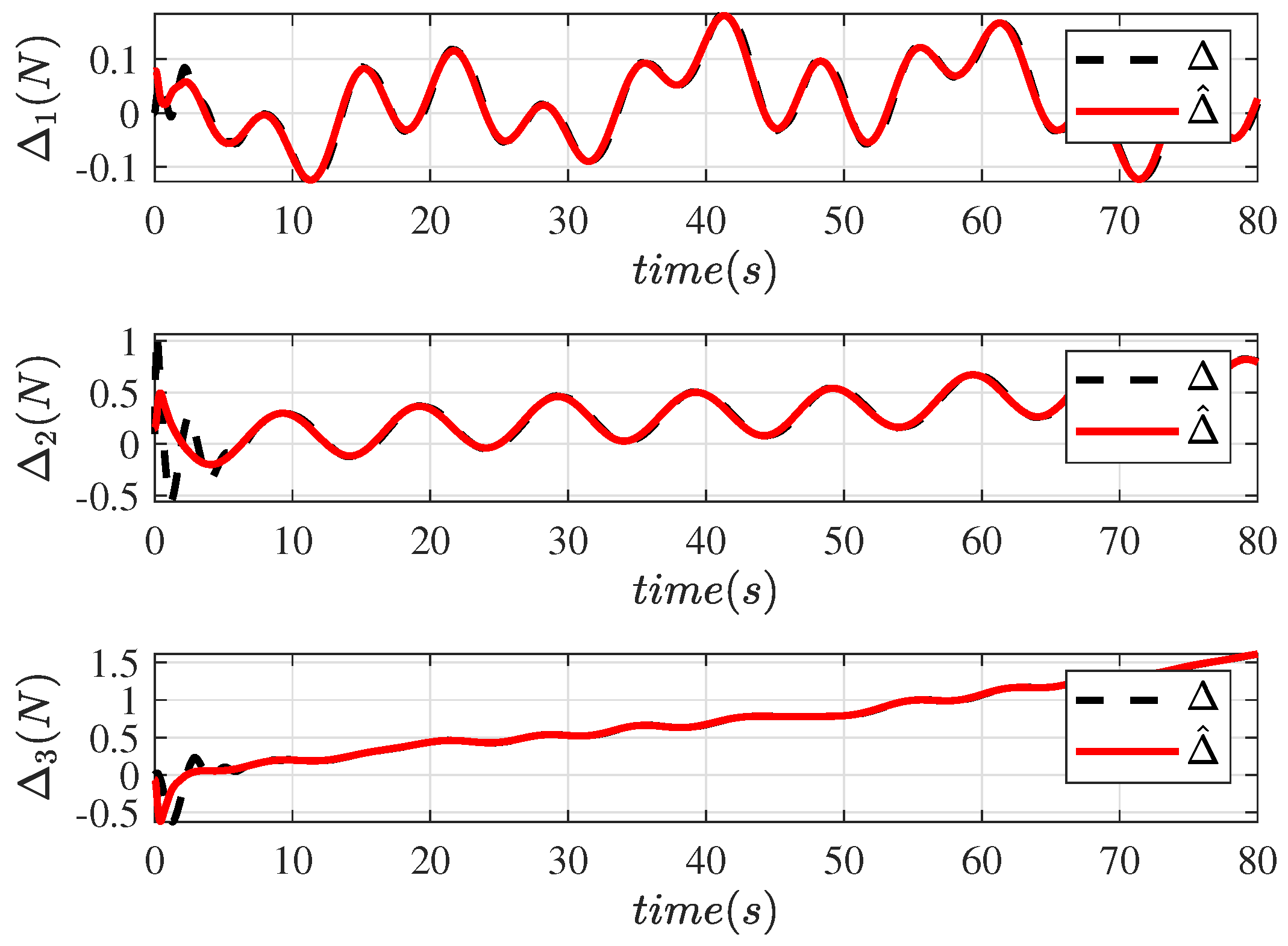
The specific results of the comparative simulation experiments are shown in Figure 3, Figure 4, Figure 5, Figure 6, Figure 7, Figure 8, Figure 9, Figure 10, Figure 11, Figure 12, Figure 13, Figure 14 and Figure 15. Figure 3, Figure 4, Figure 5 and Figure 6 show the disturbance observation performance of the proposed FT-DO, which demonstrated that the designed FT-DO could quickly and accurately handle the lumped uncertainty terms $\mathbf{\Delta }$ and ${\mathbf{\Delta }}_i$. Specifically, in Figure 3 and Figure 5, the black line represents the actual set disturbance curve, and the other line is the observation of the FT-DO, which clearly demonstrates that the designed FT-DO could stably identify disturbances in real time.

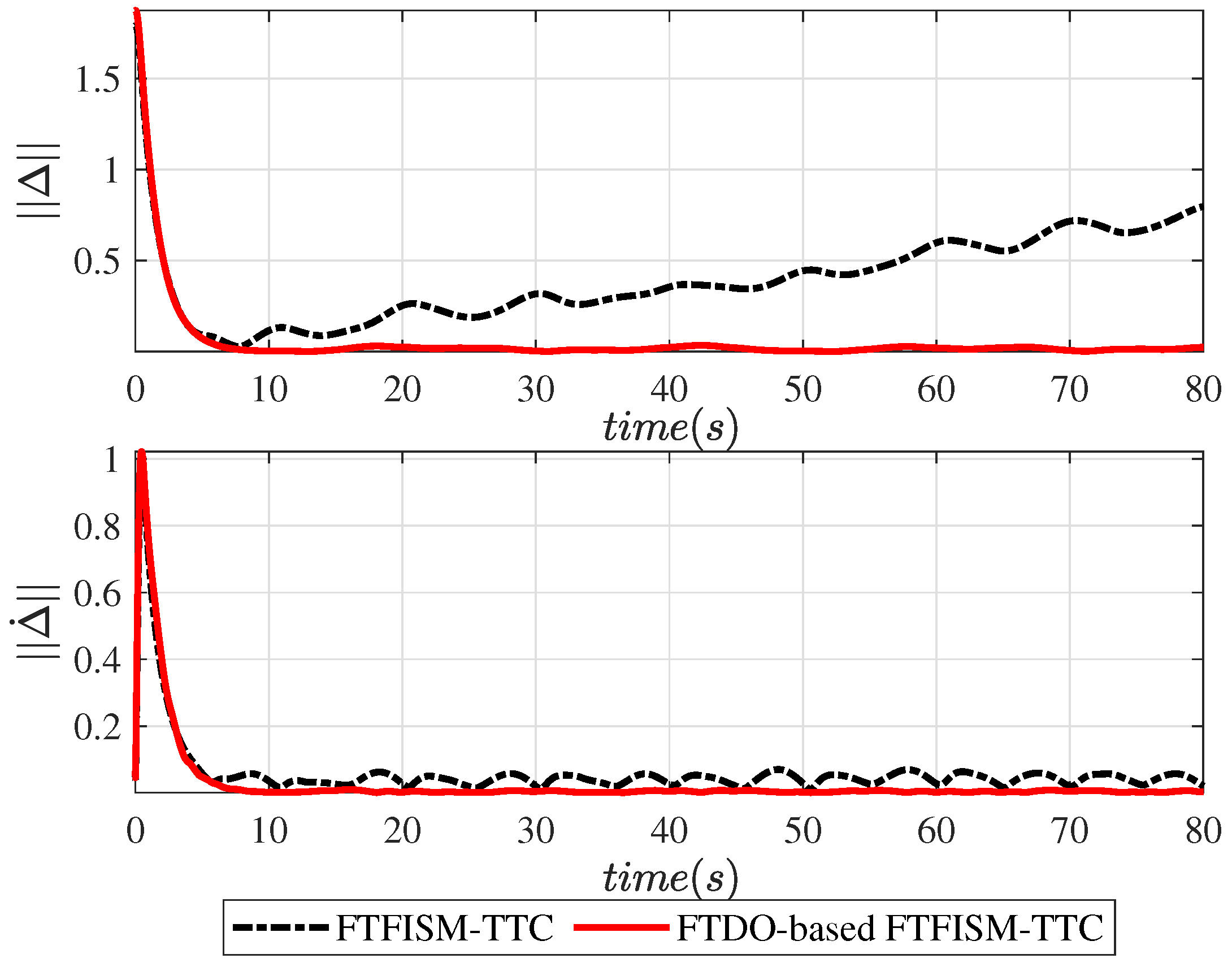
To further demonstrate the superiority of the designed disturbance observer, the norms of the disturbance identification errors are shown in Figure 4 and Figure 6. the black line represents the trajectory tracking error curve without disturbance processing, and the red line represents the tracking control effect after the disturbance was identified by FT-DO. The error level is shown in

Table 4. Observation error of the FT-DO.

T	10	20	30	40	50	60	70	80
$∥\mathbf{\Delta }∥$	0.1157	0.2548	0.3180	0.3547	0.4444	0.5966	0.7173	0.7962
${∥\mathbf{\Delta }∥}_{FTDO}$	$\mathbf{0}.\mathbf{0043}$	$\mathbf{0}.\mathbf{0260}$	$\mathbf{0}.\mathbf{0049}$	$\mathbf{0}.\mathbf{0240}$	$\mathbf{0}.\mathbf{0035}$	$\mathbf{0}.\mathbf{0211}$	$\mathbf{0}.\mathbf{0067}$	$\mathbf{0}.\mathbf{0244}$
$∥\dot{\mathbf{\Delta }}∥$	0.0360	0.0274	0.0194	0.0264	0.0279	0.0275	0.0195	0.0200
${∥\dot{\mathbf{\Delta }}∥}_{FTDO}$	$\mathbf{0}.\mathbf{0019}$	$\mathbf{0}.\mathbf{0018}$	$\mathbf{0}.\mathbf{0039}$	$\mathbf{0}.\mathbf{0045}$	$\mathbf{0}.\mathbf{0019}$	$\mathbf{0}.\mathbf{0018}$	$\mathbf{0}.\mathbf{0049}$	$\mathbf{0}.\mathbf{0028}$
$∥{\mathbf{\Delta }}_i∥$	0.0689	0.2221	0.0770	0.2174	0.0714	0.2192	0.0713	0.2370
${∥{\mathbf{\Delta }}_i∥}_{FTDO}$	$\mathbf{0}.\mathbf{0053}$	$\mathbf{0}.\mathbf{0158}$	$\mathbf{0}.\mathbf{0036}$	$\mathbf{0}.\mathbf{0128}$	$\mathbf{0}.\mathbf{0035}$	$\mathbf{0}.\mathbf{0100}$	$\mathbf{0}.\mathbf{0058}$	$\mathbf{0}.\mathbf{0126}$
$∥{\dot{\mathbf{\Delta }}}_i∥$	0.0392	0.0363	0.0400	0.0381	0.0372	0.0446	0.0392	0.0486
${∥{\dot{\mathbf{\Delta }}}_i∥}_{FTDO}$	$\mathbf{0}.\mathbf{0073}$	$\mathbf{0}.\mathbf{0067}$	$\mathbf{0}.\mathbf{0056}$	$\mathbf{0}.\mathbf{0070}$	$\mathbf{0}.\mathbf{0060}$	$\mathbf{0}.\mathbf{0062}$	$\mathbf{0}.\mathbf{0062}$	$\mathbf{0}.\mathbf{0080}$

, which further demonstrates the excellent disturbance identification ability of the proposed FT-DO.

In order to verify the excellent performance of the designed single-USV trajectory tracking controller (FTFISM-TTC), the initial states of the desired trajectories and the USV are shown in

Table 5. Initial states of the desired trajectory and the single tracking USV.

Parameters	Values	Parameters	Values
${\eta }_d\left(0\right)-$ Figure 7	${[0,-10,0]}^{\mathrm{T}}$	${\nu }_d\left(0\right)-$ Figure 7	${\left[0,0,0\right]}^{\mathrm{T}}$
${\eta }_{\mathrm{USV}}\left(0\right)-$ Figure 7	${\left[0,0,0\right]}^{\mathrm{T}}$	${\nu }_{\mathrm{USV}}\left(0\right)-$ Figure 7	${\left[0,0,0\right]}^{\mathrm{T}}$
${\eta }_d\left(0\right)-$ Figure 10	${\left[4,0,0\right]}^{\mathrm{T}}$	${\nu }_d\left(0\right)-$ Figure 10	${\left[0,0,0\right]}^{\mathrm{T}}$
${\eta }_{\mathrm{USV}}\left(0\right)-$ Figure 10	${\left[0,2,0\right]}^{\mathrm{T}}$	${\nu }_{\mathrm{USV}}\left(0\right)-$ Figure 10	${\left[0,0,0\right]}^{\mathrm{T}}$

, and the desired trajectories $T_{D,1}and{T}_{D,2}$ were set as follows:

$$\begin{array}{c}{T}_{D,1}={[6\times sin\left(0.05\times \pi \times t\right),-2\times cos\left(0.05\times \pi \times t\right),0.2\times t+2]}^{\mathrm{T}}\\ T_{D,2}={[sin\left(0.05\times \pi \times t\right)+0.15\times t,0.2\times t,0.2\times t]}^{\mathrm{T}}\end{array}$$

(47)

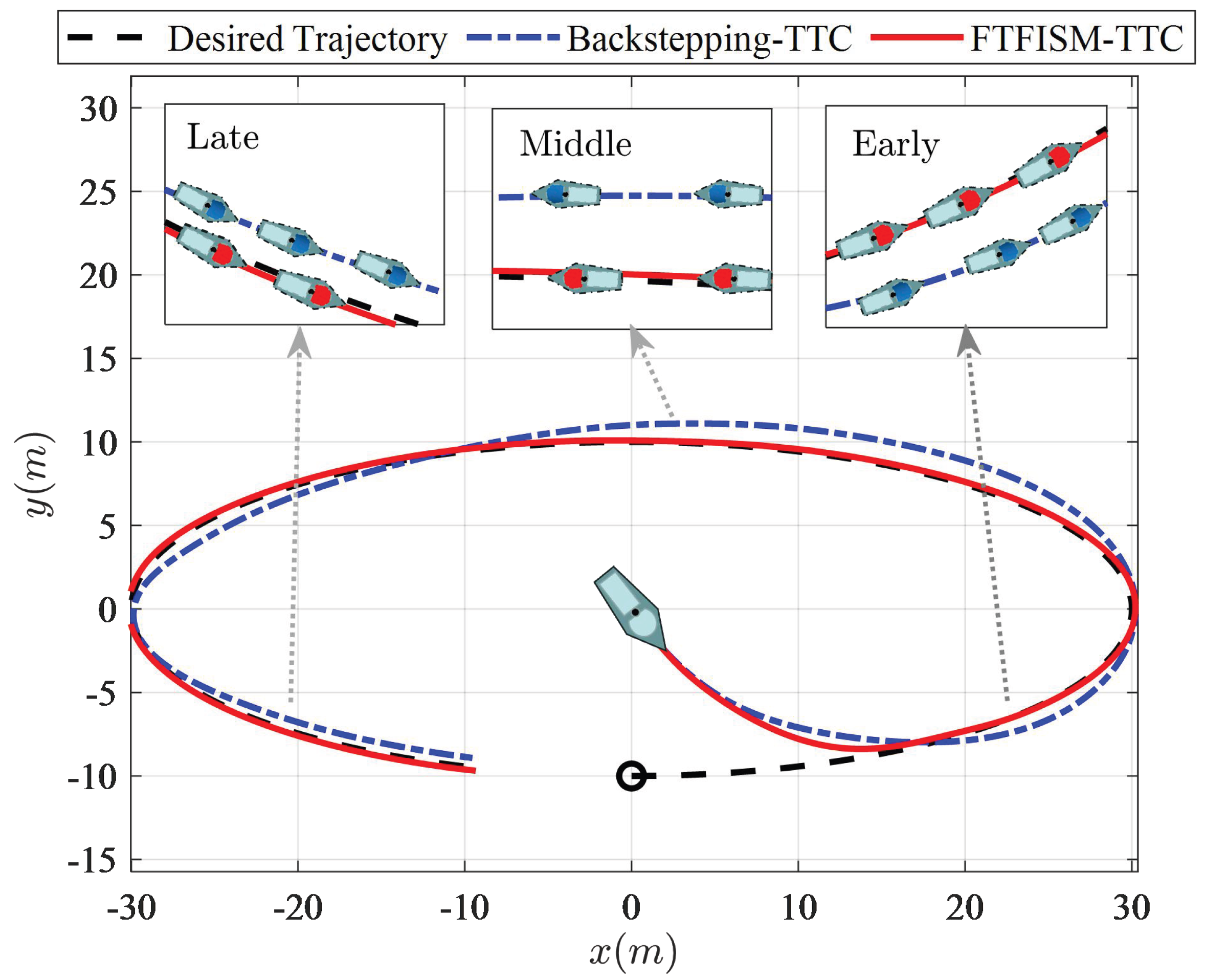
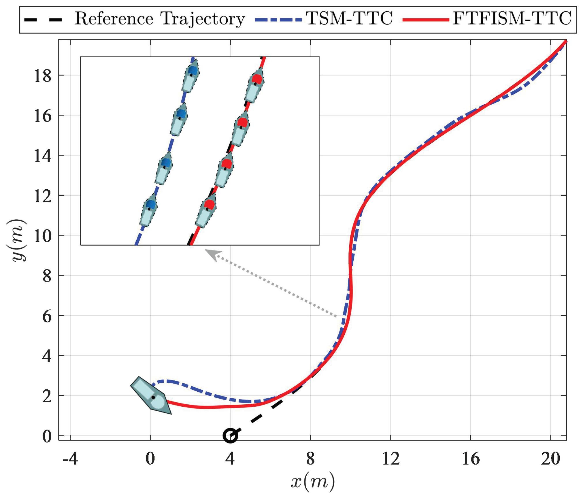
Figure 7, Figure 8, Figure 9, Figure 10, Figure 11 and Figure 12 show the comprehensive results of the simulation experiments on the FTFISM-TTC with the TSM-TTC and backstepping-TTC [25]. Specifically, in Figure 7 and Figure 10, the blue line is the tracking curve obtained with the TSM-TTC strategy and backstepping-TTC strategy, and the red line is the tracking curve obtained with the FTFISM-TTC strategy. The results show that backstepping strategy and the TSM-TTC strategy could not effectively track the expected trajectory in real time, and the proposed FTFISM-TTC had excellent tracking performance.

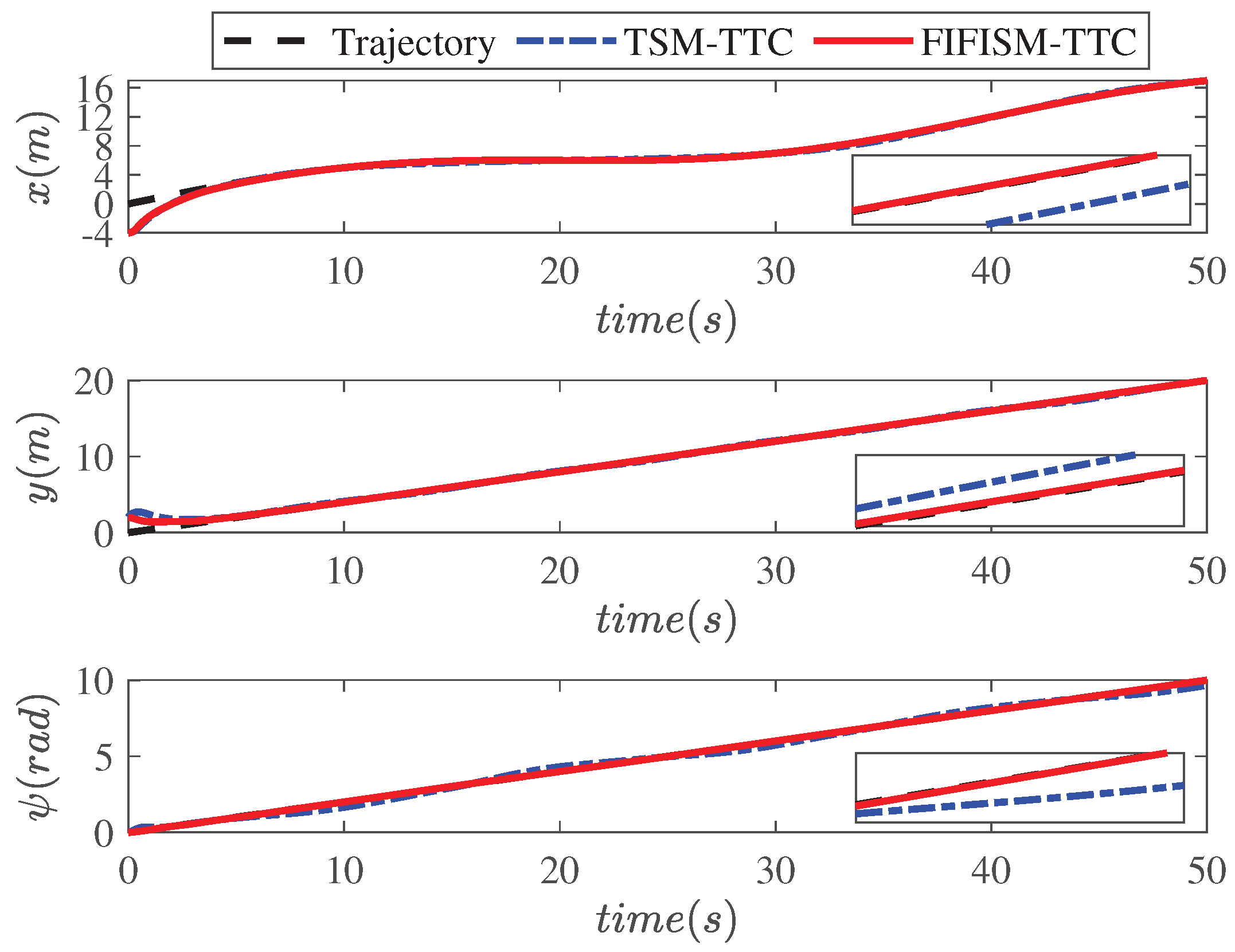
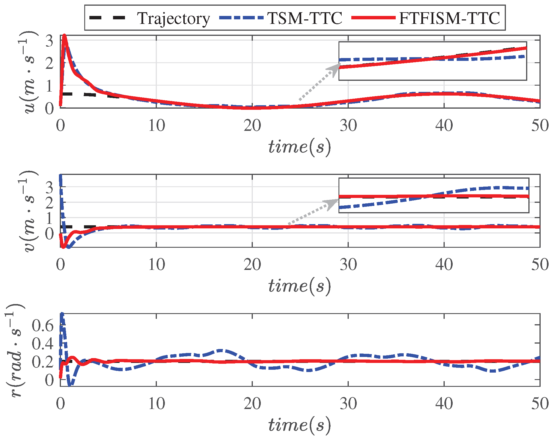
To clearly demonstrate the differences in the tracking performance of different tracking control algorithms in different dimensions, Figure 8Figure 9, Figure 11, and Figure 12 show the tracking effects on different tracking velocity and tracking position dimensions with the state-of-the-art methods and the proposed FTFISM-TTC strategy, clearly indicating that the FTFISM-TTC had more reliable tracking performance than that of TSM-TTC and backstepping-TTC.

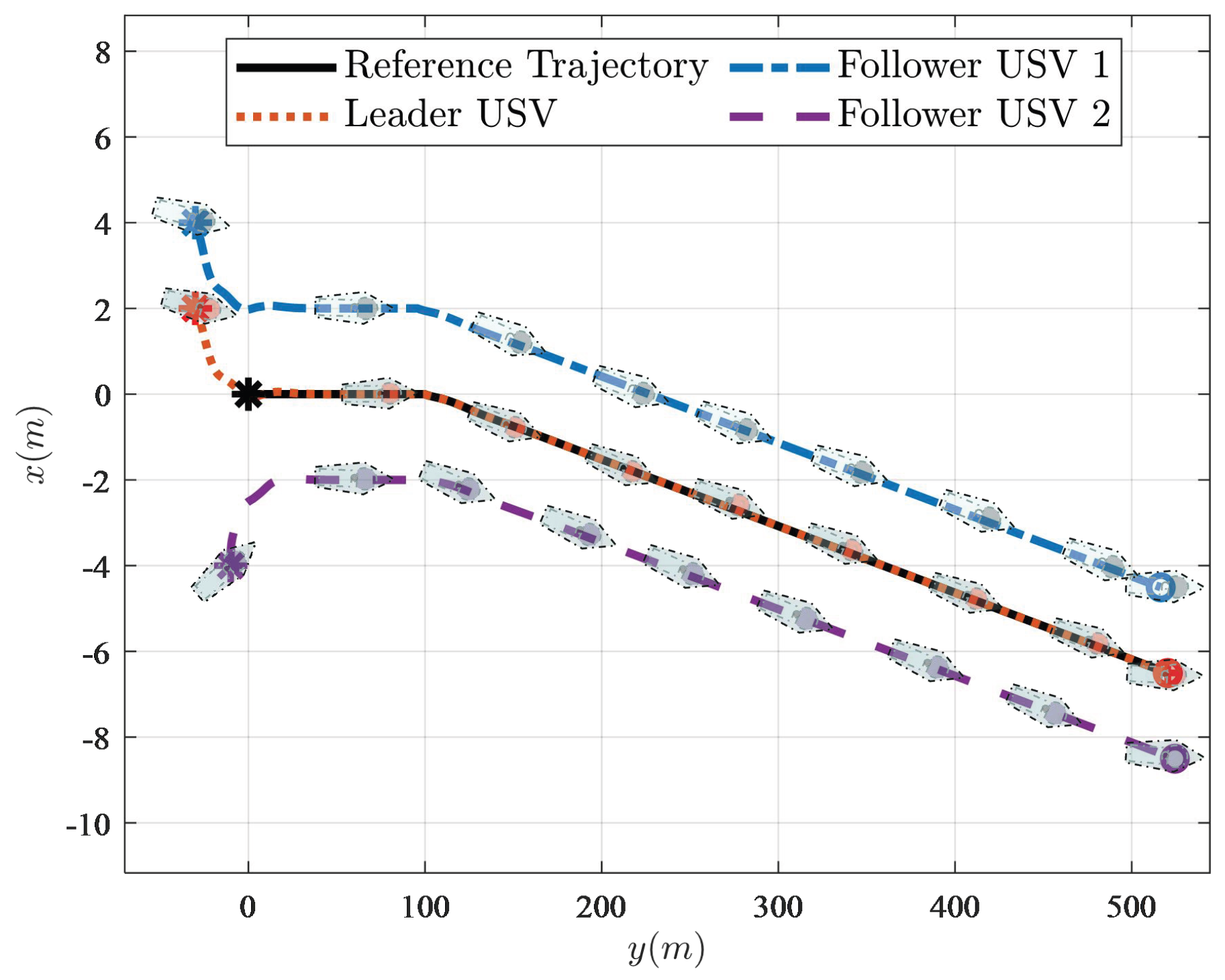
To further verify the scalability of the designed FTFISM-TTC, Figure 13 demonstrates that three USVs could continuously maintain the desired formation to achieve precise cooperative trajectory tracking. Specifically, after the leader USV navigated to the desired trajectory, the follower USVs quickly moved to the set position to ensure the desired triangular formation and steadily navigated along the desired trajectory, thus exhibiting the excellent cooperative trajectory tracking control performance of the proposed FTDO-based FTFISM-TTC strategy. The initial states of the desired trajectories and USVs are shown in

Table 6. Initial states of the three USVs.

Parameters	Values	Parameters	Values
${\eta }_d\left(0\right)$	${\left[0,0,1.5\right]}^{\mathrm{T}}$	${\nu }_d\left(0\right)$	${\left[3,0,0\right]}^{\mathrm{T}}$
${\eta }_{leaderUSV}\left(0\right)$	${\left[2,-30,0\right]}^{\mathrm{T}}$	${\nu }_{leaderUSV}\left(0\right)$	${\left[0,0,0\right]}^{\mathrm{T}}$
${\eta }_{followerUSV1}\left(0\right)$	${\left[4,-30,0.2\right]}^{\mathrm{T}}$	${\nu }_{followerUSV1}\left(0\right)$	${\left[0,0,0\right]}^{\mathrm{T}}$
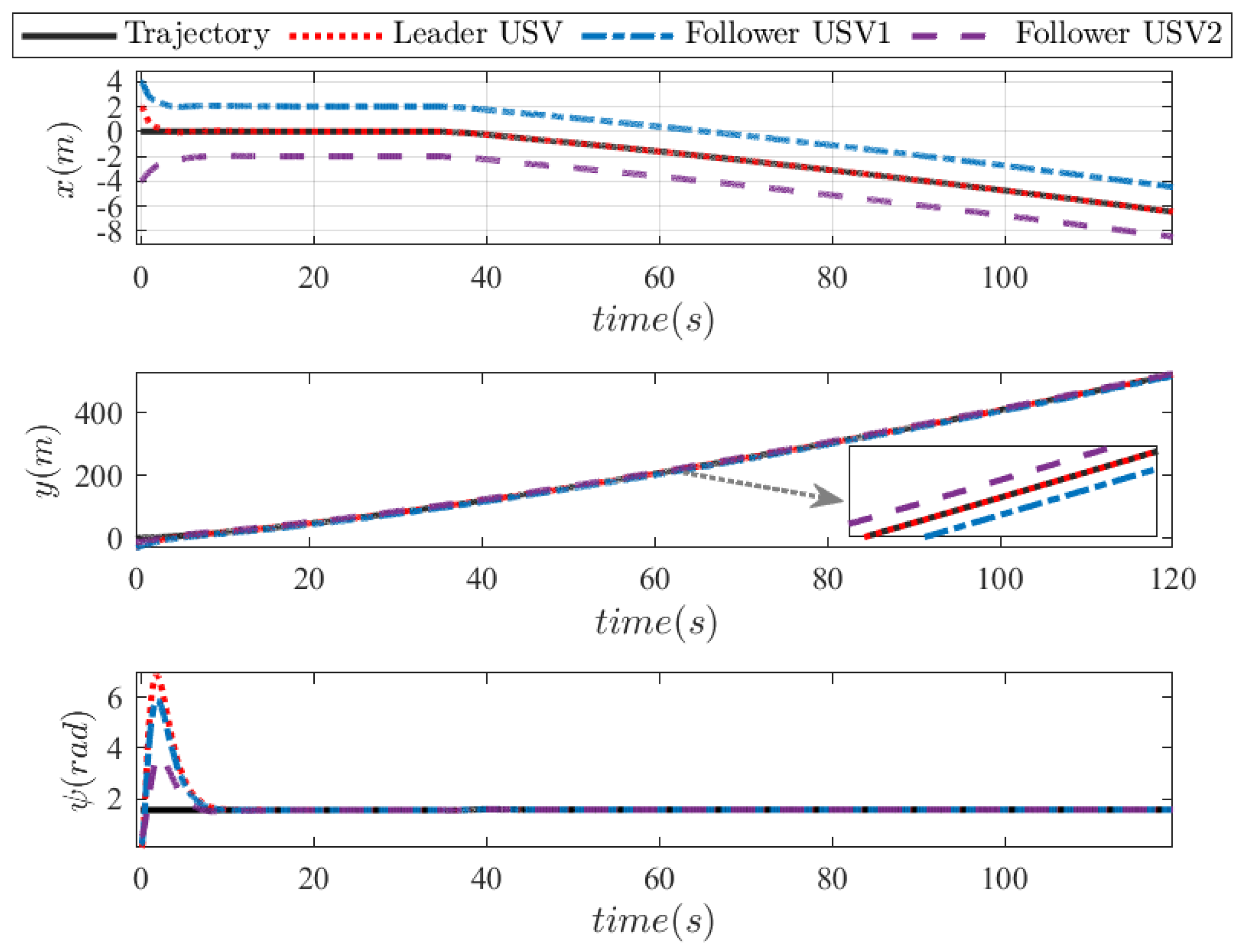
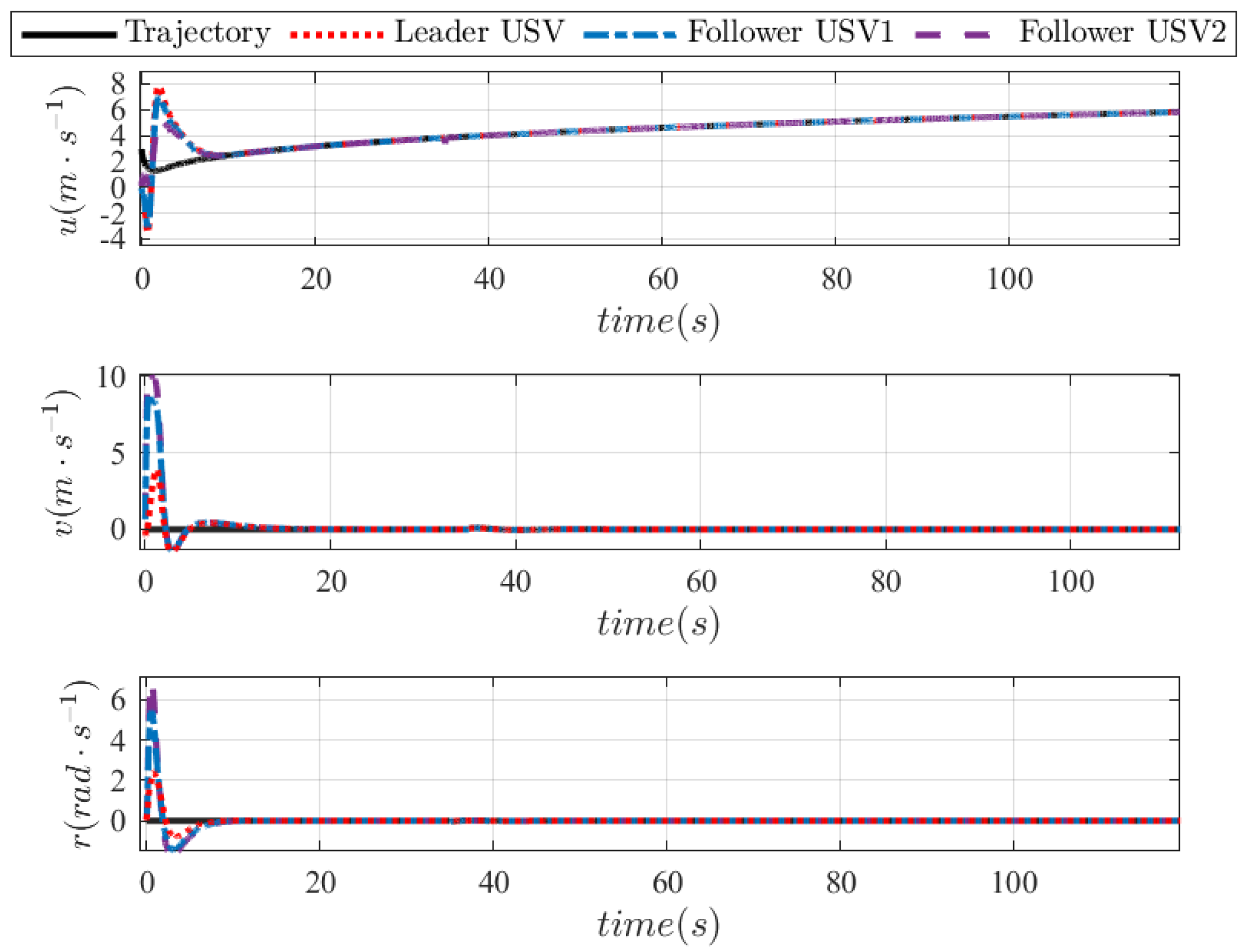
${\eta }_{followerUSV2}\left(0\right)$	${[-4,-10,0.5]}^{\mathrm{T}}$	${\nu }_{followerUSV2}\left(0\right)$	${\left[0,0,0\right]}^{\mathrm{T}}$

. For further analysis, Figure 14 and Figure 15 show the detailed position tracking curves and velocity tracking curves during cooperative trajectory tracking control, which effectively verified that the proposed FTDO-based FTFISM-TTC had strong robustness and could stably expand to the collaborative control of multiple USVs. It is worth emphasizing that the FT-DO and FTFISM-TTC proposed in this article have excellent disturbance identification ability and precise trajectory tracking performance, but still have the following limitations: due to the rigid structure limitations of the leader–follower cooperative trajectory tracking framework, the overall formation lacks flexibility, and the scalability of the algorithm needs to be further improved. Secondly, the disturbance settings in this article have certain limitations, as there are various static and dynamic obstacles that cannot be ignored in the actual marine environment, which seriously affect the safe navigation of the USV. This article provides a great research direction for precise trajectory tracking of USVs.

5. Conclusions

In motion trajectory tracking for USVs, internal model uncertainties and external environmental disturbances seriously affect the tracking accuracy. For multiple-USV cooperative trajectory tracking control with complex disturbances, a novel tracking controller was designed based on fixed-time theory and integral sliding-mode control. In the disturbance identification subsystem, a fixed-time convergent disturbance observer (FT-DO) was designed to achieve continuous and accurate observation of the lumped disturbance term and effectively eliminate the impact of initial disturbance observation errors on the observation accuracy. Then, a fixed-time-convergence fast integral sliding-mode trajectory tracking controller (FTFISM-TTC) was designed to ensure that the USV could quickly and stably track the desired trajectory and further optimize the convergence speed and tracking accuracy. Moreover, the extremely strong scalability of the proposed FTFISM-TTC was further demonstrated in multiple-USV cooperative trajectory tracking control. A rigorous stability analysis using the Lyapunov stability theory and comprehensive simulation experiments proved that the designed FT-DO and FTFISM-TTC could ensure convergence within a fixed time, and the controller’s performance was superior to that of state-of-the-art methods, such as TSM and backstepping.

Future research will focus on improving the disturbance identification accuracy and the avoidance of dynamic and static obstacles. After a rigorous theoretical demonstration and comprehensive verification through simulations, in the future, experiments with real USVs will be conducted if the experimental conditions allow.

References

1. Peng, Y.; Li, Y. Autonomous Trajectory Tracking Integrated Control of Unmanned Surface Vessel. J. Mar. Sci. Eng. 2023, 11, 568. [Google Scholar] [CrossRef]
2. Lee, J.-H.; Jeong, S.-K.; Ji, D.-H.; Park, H.-Y.; Kim, D.-Y.; Choo, K.-B.; Jung, D.-W.; Kim, M.-J.; Oh, M.-H.; Choi, H.-S. Unmanned Surface Vehicle Using a Leader–Follower Swarm Control Algorithm. Appl. Sci. 2023, 13, 3120. [Google Scholar] [CrossRef]
3. Xu, H.; Zhang, X.K. Tracking Control of Ship at Sea based on MPC with Virtual Ship Bunch under Frenet Frame. Ocean Eng. 2022, 247, 110737. [Google Scholar]
4. Yang, T.T.; Zhang, P.F.; Chen, H.Y. Distributed Prescribed-Time Leader–Follower Formation Control of Surface Vehicles with Unknowns and Input Saturation. Ocean Eng. 2023, 134, 16–27. [Google Scholar] [CrossRef]
5. Song, H.; Hu, S.; Jiang, W.; Guo, Q.; Zhu, M. Artificial Potential Field-Based Multi-UAV Formation Control and Target Tracking. Int. J. Aerosp. Eng. 2022, 2022, 4253558. [Google Scholar] [CrossRef]
6. Wen, J.B.; Yang, J.C.; Li, Y.; He, J.Y.; Li, Z.J.; Song, H.B. Behavior-Based Formation Control Digital Twin for Multi-AUG in Edge Computing. IEEE Trans. Netw. Sci. Eng. 2022, 1–11. [Google Scholar] [CrossRef]
7. Zhen, Q.Z.; Wan, L.; Li, Y.L.; Jiang, D.P. Formation Control of A Multi-AUVs System based on Virtual Structure and Artificial Potential Field on SE(3). Ocean Eng. 2022, 253, 111148. [Google Scholar] [CrossRef]
8. Pang, W.; Zhu, D.Q.; Liu, C.X.; Wang, L.L. The Multi-AUV Time-Varying Formation Reconfiguration Control based on Rigid-Graph Theory and Affine Transformation. Ocean Eng. 2023, 270, 113521. [Google Scholar] [CrossRef]
9. Wang, D.; Kong, M.; Zhang, G.; Liang, X. Adaptive Second-Order Fast Terminal Sliding-Mode Formation Control for Unmanned Surface Vehicles. J. Mar. Sci. Eng. 2022, 10, 1782. [Google Scholar] [CrossRef]
10. Liu, Z.; Cai, W.; Zhang, M.; Lv, S. Improved Integral Sliding Mode Control-Based Attitude Control Design and Experiment for High Maneuverable AUV. J. Mar. Sci. Eng. 2022, 10, 795. [Google Scholar] [CrossRef]
11. Nguyen, N.P.; Park, D.; Ngoc, D.N.; Xuan-Mung, N.; Huynh, T.T.; Nguyen, T.N.; Hong, S.K. Quadrotor Formation Control via Terminal Sliding Mode Approach: Theory and Experiment Results. Drones 2022, 6, 172. [Google Scholar] [CrossRef]
12. Souissi, S.; Boukattaya, M. Time-Varying Nonsingular Terminal Sliding Mode control of Autonomous Surface Vehicle with predefined convergence time. Ocean Eng. 2022, 263, 112264. [Google Scholar] [CrossRef]
13. Oliveira, T.R.; Melo, T.G.; Hsu, L.; Cunha, J.P.V.S. Monitoring Functions Applied to Adaptive Sliding Mode Control for Disturbance Rejection. IFAC Papers-OnLine 2017, 50, 2684–2689. [Google Scholar] [CrossRef]
14. Hsu, L.; Oliveira, T.R.; Cunha, J.P.V.; Yan, L. Adaptive Unit Vector Control of Multivariable Systems Using Monitoring Functions. Int. J. Robust Nonlinear Control 2019, 29, 583–600. [Google Scholar] [CrossRef]
15. Wang, N.; Deng, Z.C. Finite-time Fault Estimator based Fault-Tolerance Control for A Surface Vehicle with Input Saturations. IEEE Trans. Ind. Inform. 2020, 16, 1172–1181. [Google Scholar] [CrossRef]
16. Wang, N.; Karimi, H.R. Successive Waypoints Tracking of An Underactuated Surface Vehicle. IEEE Trans. Ind. Inform. 2020, 16, 898–908. [Google Scholar] [CrossRef]
17. Wang, N.; Su, S.F. Finite-time Unknown Observer-based Interactive Trajectory Tracking Control of Asymmetric Underactuated Surface Vehicles. IEEE Trans. Control Syst. Technol. 2021, 29, 794–803. [Google Scholar] [CrossRef]
18. Chen, D.; Zhang, J.; Li, Z. A Novel Fixed-Time Trajectory Tracking Strategy of Unmanned Surface Vessel Based on the Fractional Sliding Mode Control Method. Electronics 2022, 11, 726. [Google Scholar] [CrossRef]
19. Vo, A.T.; Truong, T.N.; Kang, H.J. A Novel Fixed-Time Control Algorithm for Trajectory Tracking Control of Uncertain Magnetic Levitation Systems. IEEE Access 2021, 9, 47698–47712. [Google Scholar] [CrossRef]
20. Polyakov, A. Nonlinear Feedback Design for Fixed-Time Stabilization of Linear Control Systems. IEEE Trans. Automat. Control 2012, 57, 2106–2110. [Google Scholar] [CrossRef] [Green Version]
21. Liu, W.; Ye, H.; Yang, X. Super-Twisting Sliding Mode Control for the Trajectory Tracking of Underactuated USVs with Disturbances. J. Mar. Sci. Eng. 2023, 11, 636. [Google Scholar] [CrossRef]
22. Gu, N.; Peng, Z.H.; Wang, D.; Liu, L.; Jiang, Y. Nonlinear Observer Design for A Robotic Unmanned Surface Vehicle with Experiment Results. Appl. Ocean. Res. 2020, 95, 102028. [Google Scholar] [CrossRef]
23. Wang, N.; Zhu, Z.; Qin, H.; Deng, Z.; Sun, Y. Finite-Time Extended State Observer-based Exact Tracking Control of An Unmanned Surface Vehicle. Int. J. Robust Nonlinear Control 2021, 31, 1704–1719. [Google Scholar] [CrossRef]
24. Wang, N.; Ki Ahn, C. Hyperbolic-Tangent LOS Guidance-Based Finite-Time Path Following of Underactuated Marine Vehicles. IEEE Trans. Ind. Electron. 2020, 67, 8566–8575. [Google Scholar] [CrossRef]
25. Lu, L.; Dan, W.; Peng, Z.H. Eso-based Line-of-Sight Guidance Law for Path Following of Underactuated Marine Surface Vehicles with Exact Sideslip Compensation. IEEE J. Ocean. Eng. 2017, 42, 477–487. [Google Scholar] [CrossRef]
26. Pinto, H.L.C.P.; Oliveira, T.R.; Hsu, L. Fault Reconstruction for Delay Systems via Least Squares and Time-Shifted Sliding Mode Observers. Asian J. Control 2019, 21, 52–69. [Google Scholar] [CrossRef]
27. Pinto, H.L.C.P.; Oliveira, T.R.; Hsu, L. Sliding Mode Observer for Fault Reconstruction of Time-Delay and Sampled-Output Systems-A Time Shift Approach. Automatica 2019, 106, 390–400. [Google Scholar] [CrossRef]
28. Wang, N.; He, L. Leader-Follower Formation Control of Surface Vehicles: A Fixed-Time Control Approach. ISA. Trans. 2022, 124, 356–364. [Google Scholar] [CrossRef]
29. Bhat, S.P.; Bernstein, D.S. Continuous Finite-Time Stabilization of The Translational and Rotational Double Integrators. IEEE Trans. Automat. Control 1998, 43, 678–682. [Google Scholar] [CrossRef] [Green Version]
30. Zuo, Z. Nonsingular Fixed-Time Consensus Tracking for Second-Order Multi-Agent Networks. Automatica 2015, 54, 305–309. [Google Scholar] [CrossRef]
31. Zuo, Z.; Tian, B.; Defoort, M. Fixed-Time Consensus Tracking for Multiagent Systems with High-Order Integrator Dynamics. IEEE Trans. Autom. Control 2017, 63, 563–570. [Google Scholar] [CrossRef] [Green Version]
32. Fiori, S. Model Formulation Over Lie Groups and Numerical Methods to Simulate the Motion of Gyrostats and Quadrotors. Mathematics 2019, 7, 935. [Google Scholar] [CrossRef] [Green Version]
33. Tarsi, A.; Fiori, S. Lie-Group Modeling and Numerical Simulation of a Helicopter. Mathematics 2021, 9, 2682. [Google Scholar] [CrossRef]
34. Skjetne, R.; Smogeli, Ø.; Fossen, T.I. Modeling, Identification, and Adaptive Maneuvering of Cybership II: A Complete Design with Experiments. IFAC Proc. 2004, 37, 203–208. [Google Scholar] [CrossRef]
Figure 1. (a) Cybership II USV model. (b) Earth-fixed coordinate system error and body-fixed relative coordinate system error of a USV.
Electronics 12 02896 g001
Figure 2. Cooperative trajectory tracking framework for multiple USVs.
Electronics 12 02896 g002
Figure 3. Observation results of the FTDO leader.
Electronics 12 02896 g003
Figure 4. Norm of the FTDO leader’s tracking errors and derivatives.
Electronics 12 02896 g004
Figure 5. Observation results of the FTDO follower.
Electronics 12 02896 g005
Figure 6. Norm of the FTDO follower’s tracking errors and derivatives.
Electronics 12 02896 g006
Figure 7. Trajectory tracking curve of backstepping-TTC and the FTFISM-TTC.
Electronics 12 02896 g007
Figure 8. Position tracking of backstepping-TTC and the FTFISM-TTC.
Electronics 12 02896 g008
Figure 9. Velocity tracking of backstepping-TTC and the FTFISM-TTC.
Electronics 12 02896 g009
Figure 10. Trajectory tracking curve of TSM-TTC and the FTFISM-TTC.
Electronics 12 02896 g010
Figure 11. Position tracking of TSM-TTC and the FTFISM-TTC.
Electronics 12 02896 g011
Figure 12. Velocity tracking of TSM-TTC and the FTFISM-TTC.
Electronics 12 02896 g012
Figure 13. Collaborative trajectory tracking curve of the three USVs.
Electronics 12 02896 g013
Figure 14. Position tracking of the three USVs.
Electronics 12 02896 g014
Figure 15. Velocity tracking of the three USVs.
Electronics 12 02896 g015