Investigation of the Distribution Problem in the Operating State of an Electromagnetic Railgun: Radio Fuse Disturbance, Field Characteristics, and Susceptible

Abstract

The purpose of this article is to analyze the front door coupling effect that may occur in the projectile receiver due to the discharge pulse radiation in electromagnetic railguns, and to simulate the discharge pulse interference. This phenomenon will have an impact on the launch of the projectile, causing its fuse to be disturbed, ultimately affecting the weapon performance of the electromagnetic railgun. Discharge refers to when the armature carrying the projectile is fired out of the chamber, and the armature connected between the two rails detaches, causing a circuit break in the electrical circuit during the operation of the electromagnetic railgun. The current flowing through the armature is disturbed, causing an instantaneous high voltage to penetrate the air gap between the two rails, generating nanosecond pulse width discharge voltage pulse radiation, with a spectrum of up to tens of megahertz. In this paper, we establish a receiving antenna model on the projectile, which is essentially a horn antenna, receiving electromagnetic pulses from the discharge process, and coupling the pulse interference through its front door. During the analysis and calculation, we established an antenna receiver model located in the C-band with a frequency of 6 GHz for simulation, analyzed and calculated the actual interference loaded on the projectile after front door coupling, and verified the correctness of the simulation settings and results by comparing with the literature. Finally, we found that because the main energy spectrum of the pulse is at MHz level, when the front door of the C-band horn antenna is coupled, the standing wave ratio of the antenna is very large and the gain is very small, so the pulse interference is filtered, which can make the interference finally loaded on the projectile insufficient to affect the normal operation of the projectile. At the same time, it is recommended to add an RF filter to the receiving channel to further enhance anti-interference ability, so as to ultimately enable the electromagnetic railgun to function properly.

1. Introduction

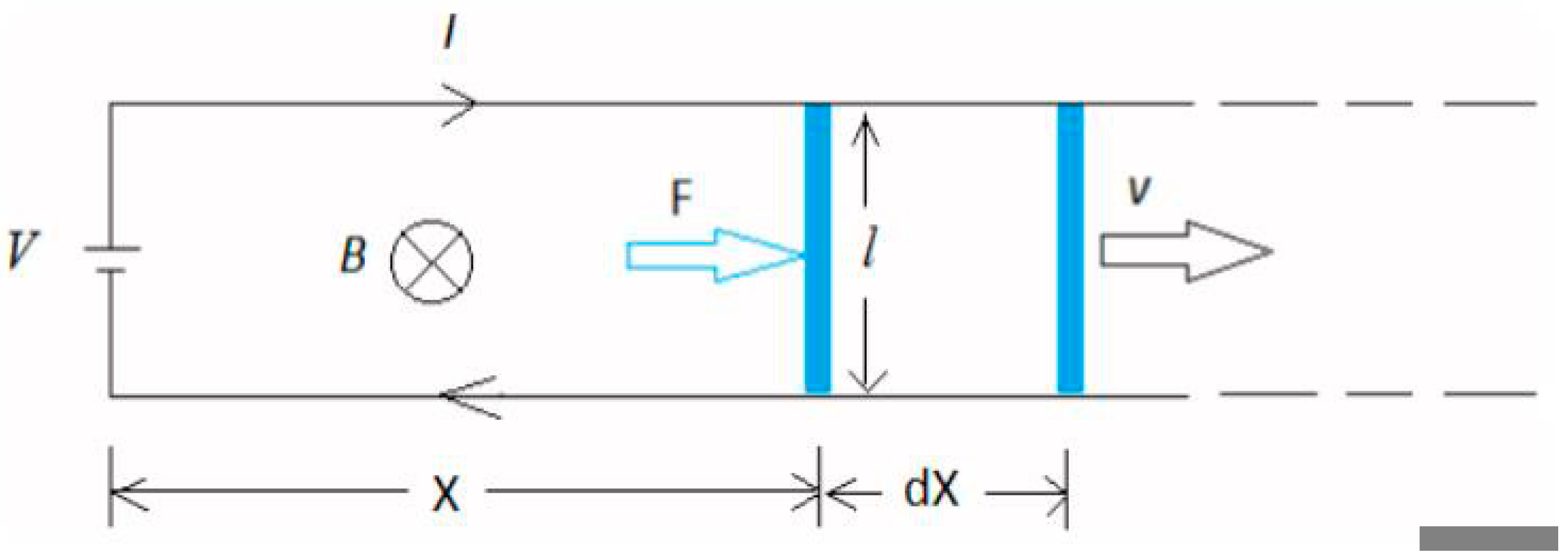
An electromagnetic railgun is a long-range, high-energy, and multitasking weapon with a high firing rate and long range, as shown in Figure 1. The electromagnetic railgun system is excited by electrical energy, with V representing the voltage of the pulse excitation source, generating a pulse current of size I that flows through the armature from one track and then back from the other track. According to the principle of electromagnetic induction, pulse current excites the magnetic field B inside the electromagnetic railgun, and under the action of the magnetic field, an ampere force F is generated on the armature with a length of l, where X represents the armature displacement and dX represents the displacement change. The arrows in Figure 1 represent the direction of Lorentz force and the direction of armature motion. The armature carrying the projectile is launched along the guide rail at a very high speed v, and finally, the electric fuse is manually controlled to cause the projectile to explode at the specified position, in order to achieve the goal of destroying the target object. However, electromagnetic artillery shells will generate electromagnetic pulse interference at the moment of firing from the muzzle, which will be coupled through the front door of the receiver on the projectile, thereby affecting the projectile fuse. If the interference intensity is too large, it will cause the projectile to explode in advance, making the electromagnetic railgun unable to function. Therefore, we need to design the receiver model reasonably and filter the received pulse interference excitation, so that the interference after coupling through the front door will not have a serious impact on the projectile and can enable the electromagnetic railgun to launch normally.

Our research objective was to simulate the electromagnetic pulse interference generated by the electromagnetic track railgun projectile at the time of firing out of the chamber. We used HFSS tool software to obtain the coupling results after passing through our designed receiving antenna. The intermediate results obtained in the simulation can be compared with existing literature to prove the correctness of our simulation.

Through the simulation of interference, we can specifically depict the physical phenomena that occur when electromagnetic railguns are fired, simulate interference from both qualitative and quantitative perspectives, and analyze the impact of interference. In the future, others can design specific devices or load other devices based on our results to reduce the impact of interference, so that electromagnetic railguns can function normally. Otherwise, this type of pulse interference not only causes electromagnetic compatibility issues with numerous electronic devices outside the electromagnetic railgun but also has an impact on the radio fuse of the projectile due to excessive electromagnetic pulse interference, causing it to detonate in advance, at the moment of firing, thereby failing to achieve the goal of the electromagnetic railgun detonating at a fixed point.

2. Literature Review

Many scholars have studied and discussed the electromagnetic pulse interference radiation phenomena that occur in an electromagnetic railgun at the moment when the projectile accelerates its discharge from the chamber. Shen et al. focused on the electromagnetic wave emitted by the electromagnetic railgun to study the interference caused by other electronic equipment on a naval vessel. The firing process and physical mechanism of the electromagnetic railgun projectile were analyzed in detail. The authors pointed out that when an electromagnetic railgun fires a projectile out of its chamber, it creates a conductive channel at the muzzle, which is considered to radiate electromagnetic interference outward from a virtual antenna. At the same time, they classified four cases according to different plasma morphologies and plasma characteristic frequencies, and calculated the far-field electromagnetic radiation mode and the near-field electric field intensity using the GEMS simulation tool based on the principle of finite-difference time-domain. Finally, through the analysis of simulation results, the study pointed out that plasma is not an effective radiator, and the electromagnetic radiation at the later stage of emission is not as strong as that during the process of emission. In another one of their articles, the authors listed the various electromagnetic excitations with different time-domain widths that exist during the operation of the electromagnetic railgun and identified the magnitude and spectrum widths under different discharge conditions. In this paper, four different models of electromagnetic railguns are built for the pulse excitation source, and the same index is calculated as in the previous one. The main purpose is to improve the previous analysis and simulation of various electromagnetic excitation sources in the electromagnetic railgun [1,2]. In order to estimate the radiation interference caused by the discharge, F. Canavero et al. established a model of the breakdown phenomenon between the two tracks of the electromagnetic railgun. Combining the model and the specific discharge process, the electric and magnetic fields were simulated at different locations around the model at different times after the start of discharge. The final result obtained the corresponding time-domain waveform and explained that the electromagnetic interference could be generated during the arc combustion phase of the railgun. However, the authors also point out that the numerical values used for this simulation are not representative and highly accurate, so a more accurate theoretical estimation of the numerical values used for simulation is an improved direction [3]. Dwyer et al. analyzed the feasibility of using the plasma generated by gas discharge as an antenna. From an experimental point of view, they observed how laser guidance and discharge produced plasma, which was then used as an antenna for transmission and reception. This paper describes specific experimental equipment and presents various data parameters of plasma generated by air discharge breakdown, which is helpful as a reference for our own simulation setup [4]. Parker et al. analyzed the electromagnetic interference caused by the armature emitted from the electromagnetic railgun muzzle. They did so by designing an inductive muzzle shunt and choosing an appropriate inductance value to make the current flowing through the armature equal to zero so that the current before and after the muzzle exit does not have the effect of breaking, thus reducing the influence of the muzzle arc on the structure of the electromagnetic railgun itself, the energy loss, and the launch track [5]. In order to solve the radiation interference caused by the muzzle, in addition to the muzzle inductance shunt method mentioned above, R.L. Fuller et al. constructed a reverse current compensation path by designing the muzzle shunt resistance to offset the current of the main circuit in order to minimize the total current [6]. Qiang et al. analyzed the electromagnetic field of the electromagnetic track railgun under dynamic conditions. They proposed a numerical calculation method. Using the measured dynamic experimental data, they calculated the current density values and the distribution characteristics of the electromagnetic field in some areas. By analyzing the data, they obtained some characteristics of the electromagnetic track railgun under dynamic conditions. At the same time, their research results on the electromagnetic fields of electromagnetic guns will be helpful for future applications in electromagnetic shielding design [7]. After understanding the basic physical processes of the generation of pulse interference, we turn our attention to the literature describing the process of the generation of the interference, which can help us to analyze the pulse interference qualitatively. Bernardes et al. studied the generation of pulses from the energy perspective of the overall electromagnetic railgun system. They pointed out that the PPS power supply charges the inductance, and the whole circuit has a large current flowing through it. When the current is interrupted, a very high amplitude muzzle voltage is added to both ends of the muzzle to break through the gap, resulting in pulse interference [8]. Yong et al. proposed that the muzzle arc would be generated when the electromagnetic track railgun fired from the muzzle, which was caused by the high voltage formed at both ends of the muzzle after the muzzle was released. The authors then studied how to eliminate this kind of muzzle arc to avoid its adverse effects [9]. L. Gharib et al. also pointed out that when the armature accelerates through the bore to the muzzle, it emits the bore. A high-pressure breakdown gap between the two tracks of the electromagnetic railgun creates a plasma gap between the two tracks, which also creates electromagnetic radiation interference. It can be seen here as a virtual antenna that releases the energy stored in the electromagnetic railgun. Electromagnetic interference affects the electromagnetic characteristics of the external equipment and causes adverse effects [10,11].

3. Methodology

In our study, the research goal was to simulate the electromagnetic pulse interference generated. The specific implementation method was to depict the pulse interference through a clear physical mechanism, and then compare the intermediate results used in HFSS simulation with existing literature simulation results to verify the correctness of our simulation results. Unlike existing literature, we highlight the analysis and simulation of electromagnetic pulse interference generated by discharge through the front door coupling effect of the designed antenna, rather than just analyzing the mechanism of electromagnetic pulse interference generated during the electromagnetic railgun firing process. Based on existing literature, the similarity lies in the analysis and research of the specific principle of electromagnetic pulse interference, that is, how to generate discharge during the firing process of electromagnetic guns, leading to the excitation of pulse interference. At the same time, the induction and organization of the types and magnitudes of electromagnetic excitation inside electromagnetic guns in the literature also provide us with assistance in a clearer understanding of various phenomena and their causes. The innovation of this article lies in starting from the performance of the electromagnetic railgun itself so that the electromagnetic railgun projectile can be launched normally. The pulse interference generated by the simulation is coupled through the design of the front door of the antenna, providing further assistance for others to think about how to reduce the impact of pulse interference and avoid interference in the future. So, our focus is on studying the electromagnetic pulse interference generated during the simulation of an electromagnetic railgun discharge. In the simulation tool HFSS, coupling occurs through the designed receiving antenna, and the intermediate results used in the simulation are compared with the literature to demonstrate the correctness of the simulation interference.

When the railgun head is powered by a pulse power supply (PPS), the generated current flows in from one rail of the electromagnetic railgun, passes through the conductive armature, and then flows back from the other rail, forming a basic electrical circuit. When there is a current flowing through the armature, it is known from the characteristics of the pulse power supply that a changing current can be generated. According to the law of electromagnetic induction, a magnetic field B is induced around it, and under the action of Ampere force, the armature can move in a directional direction toward the muzzle of the electromagnetic railgun. The schematic diagram of the rail gun principle is shown in Figure 2, where w represents the width of the rail and h represents the height of the rail. The red arrow in Figure 2 represents the direction of the current I and the black arrow represents the direction of the Lorentz force F.

When the armature carrying the projectile is fired out of the chamber, electromagnetic pulse interference will be generated, causing interference to the radio fuse on the projectile and affecting the function of the electromagnetic gun. The process of generating a disturbance source for a projectile radio fuse is as follows: after the pulse power supply starts to supply power, the armature moves toward the muzzle under the action of Ampere force F. When it moves to the muzzle, it is fired out, creating a high-voltage breakdown gap between the two tracks of the electromagnetic gun, establishing a plasma gap between the two tracks, and generating electromagnetic radiation interference [7,10,11]. This phenomenon can also be called muzzle flash. Subsequently, it can be seen as a virtual antenna that releases the energy stored in the electromagnetic gun, and electromagnetic interference can affect the electromagnetic characteristics of external devices, causing adverse effects. The planar schematic diagram of the movement and exit torque of the armature in the electromagnetic gun is shown in Figure 3, where s represents the distance between the guide rails, L₁ represents the armature displacement, and L₀ represents the change in armature displacement. The position marked in light color is the state of receiving Ampere force in the gun barrel and moving to the right end of the gun barrel, while the position of the dark armature is the critical state. At this point, it will be fired out of the gun, and the electrical circuit inside the electromagnetic gun will be cut off, generating high pressure and loading at both ends of the track.

From an energy perspective, the entire energy of the electromagnetic gun is initially stored in the capacitor bank of the PPS (pulse power supply). During the process before the armature is discharged, the capacitor bank will discharge, and it usually has multiple diodes to prevent reverse charging. Because during operation the electrical circuit is in good condition and there is a strong current flowing through the armature, a large portion of the initial energy of the electromagnetic gun will be stored in the inductance of the circuit. When the armature carrying the projectile exits the chamber, the large current that originally flowed through undergoes a process of making and breaking, leading to the application of extremely high amplitude muzzle voltage at both ends of the outlet muzzle, causing the air gap between the parallel guide rails to be broken down, resulting in discharge pulses [8].

From a quantitative perspective, based on the mechanism of the pulse discharge generated by the breakdown and the accompanying characteristic phenomena of pulse discharge described above, discharge at extremely high voltage belongs to the type of spark discharge [12], generating discharge voltage pulses with a width of ns. Based on the basic characteristics of spark discharge and the gap breakdown characteristics of high voltage [13,14,15,16,17], we have determined that the time-domain width of the generated nanosecond width discharge pulse is within tens of nanoseconds (20–60 ns), with a characteristic value of 40 ns. Spark discharge is based on the streamer theory. As the voltage at both ends of the gap increases, the number of electron avalanches between the air gaps increases. When the breakdown threshold is exceeded, streamer conduction is formed, and spark discharge begins [13]. The gap breakdown voltage of spark discharge is very high, around tens or hundreds of kilovolts. The theory of breakdown field strength and corresponding breakdown voltage of spark discharge is not particularly complete, and their values are related to the specific gap type and uniformity. In the electromagnetic gun environment studied in this article, the gap at the muzzle is a flat gap with a symmetrical structure. Therefore, it can be inferred from existing conclusions that the gap belongs to a uniform or slightly non-uniform type. The breakdown field strength of the air gap is 30 kv/cm, and the non-uniformity coefficient can be taken as 1.0. Therefore, the breakdown voltage threshold can be obtained by U = Ed (d is the gap distance). When the voltage at both ends reaches the breakdown voltage threshold, a spark discharge gap is broken down, forming a highly conductive channel, similar to a short circuit. There is a large amount of current passing through the channel, and then the voltage drops sharply [14]. At this point, a discharge radiation pulse will be generated, and the curve is considered to be in the form of a voltage pulse. Based on the principle of the breakdown process mentioned above, the voltage between the two rails reaches a peak value and then rapidly decreases, forming a pulse interference [18]. After a period of current retention at the discharge point of the muzzle, without an arc extinguishing device, the muzzle will transition from a very short initial spark discharge to an arc state.

Our main focus is on the interference caused by the initial nanosecond pulse radiation on the radio fuse in a very short period of time, and our work mainly consists of simulating the pulse radiation interference.

4. Simulation Settings

For the projectile receiver, we establish a simulation model in HFSS (high-frequency structure simulator) to analyze the coupling effect of specific antenna models on the generated discharge pulse radiation interference. The antenna model of the receiver was established in the specified frequency band, meeting the requirements of general traveling wave characteristics. At the same time, theoretical radiation interference excitation was added to obtain the coupling output result.

We utilize the transient solution mode of HFSS to directly express pulse interference in the time domain for simulation. Its disadvantage is that the solution mode of HFSS needs to be transformed, but the advantages are more obvious. By using the transient mode, the pulse interference form obtained through the theory described in the literature can be directly added to the excitation of the antenna, and it can display both time-domain and frequency-domain expressions, thus starting the simulation process and obtaining the final results.

For the implementation of the scheme, the first step is to convert the HFSS solution mode. When verifying the basic characteristics of the designed antenna, such as the S-parameter, it is necessary to perform in the driven modal solution mode, while to obtain coupling results in the subsequent simulation process, the transient solution mode should be used. The difficulty lies in the comparison and verification of the results. After determining the pulse to be added to the simulation, we need to compare the intermediate results used with the results in the literature to prove the reliability of the simulation. This involves carefully analyzing the model described in the reference literature, and even delving deeper into the circuit level to fully discuss and test the uncertain aspects in the description, so as to reproduce and analyze this model more completely. After sufficient discussion, the analysis results of the model described in the literature can be obtained. Finally, we analyze and compare the relatively complete results with the results presented in the literature to draw a conclusion.

Based on the research background and an introduction to the physical mechanism of the entire operation process of the electromagnetic gun, we needed to set up a suitable receiving antenna model on the projectile to couple the electromagnetic pulse radiation generated during the bore-out process, so that the final effect on the projectile electric fuse is of small amplitude and will not cause the fuse to detonate. The antenna is located on the projectile exiting the chamber, and the specific model position and process status are shown in Figure 4 below. The electromagnetic pulse interference generated at the moment of exit will enter through the front door of the receiving antenna we have designed.

When a large pulsed current flows from the current source into a guide rail, passes through the armature, and then flows back to the current source from another guide rail, a “current source guide rail armature” closed circuit is formed, as shown in Figure 4. According to Ampere’s loop law, the large pulsed current $I$ induces a transient strong magnetic field $B$ between the guide rail and the armature, and one obtains

$$\overrightarrow{B}=\frac{{\mu }_{0}I}{4\pi r_0}=\frac{{\mu }_0}{4\pi }\cdot {\displaystyle {\iiint }_V\left(\frac{\overrightarrow{J}({\overrightarrow{r}}^{\prime })\times (\overrightarrow{r}-{\overrightarrow{r}}^{\prime })}{{\left|\overrightarrow{r}-{\overrightarrow{r}}^{\prime }\right|}^2}\right)}dV$$

(1)

where $\overrightarrow{J}({\overrightarrow{r}}^{\prime })$ is the current density and ${\mu }_0$ is the vacuum magnetic permeability. At this point, the pulsed high current $I$ on the armature reacts with the magnetic field of the guide rail to generate an ampere force $\overrightarrow{F}$, as shown in Equation (2), pushing the armature and the projectile placed in front of the armature to accelerate along the guide rail, thereby achieving a high muzzle initial velocity for remote launch.

$$\overrightarrow{F}=m\frac{dv}{dt}={\displaystyle \underset{L}{\int }d\overrightarrow{F}={\displaystyle \underset{L}{\int }Id\overrightarrow{l}\times \overrightarrow{B}}}$$

(2)

According to Newton’s second law, it can be inferred that

$$\overrightarrow{s}(t)=\frac{1}{m}{\displaystyle \iint \overrightarrow{F}(t)d{t}^2}$$

(3)

$$\overrightarrow{v}(t)=\frac{1}{m}{\displaystyle {\int }_0^t\overrightarrow{F}(t)}dt$$

(4)

where $s$ is the armature displacement, $v$ is the armature velocity, and $m$ is the armature mass. For the transient problem of Maxwell 3D, the following method was used to add excitation sources:

$$\overrightarrow{\nabla }\times \overrightarrow{H}=\overrightarrow{J}$$

(5)

$$\overrightarrow{\nabla }\times \overrightarrow{E}=-\frac{\partial \overrightarrow{B}}{\partial t}$$

(6)

$$\overrightarrow{\nabla }\cdot \overrightarrow{B}=0$$

(7)

Based on the above three equations, it can be derived that

$$\overrightarrow{\nabla }\times \frac{1}{\sigma }\overrightarrow{\nabla }\times \overrightarrow{H}+\frac{\partial \overrightarrow{B}}{\partial t}=0$$

(8)

$$\overrightarrow{\nabla }\cdot \overrightarrow{B}=0$$

(9)

It can be seen that the final result is represented by the first-order edge elements of the vector field and the second-order nodes of the scalar field. Specifically, for solid and stranded conductors, the field equation is coupled with the circuit equation because the current is unknown when an external voltage is applied. For conductors with added voltage, the ohmic voltage drop ring on the i-th conductor can be written as

$$V_{R_i}={\displaystyle \underset{R_C\left(i\right)}{\int }{\displaystyle \iint J_{0i}\left(E+v\times B\right)}}dR$$

(10)

where $J_{0i}$ is the current density. The stranded conductor is considered to have no induced eddy currents, so it is placed in a non-conductive area. This means that in order to calculate the ohmic voltage drop, we cannot use the same steps as for solid conductors when calculating stranded conductors. At this point, we can use lumped parameters to represent the DC resistance of the winding. Since the total magnetic flux does not change, we obtain an induced voltage similar to the connection method of a solid conductor. In this way, we introduced a time-domain equation to solve the above problem, as follows:

$${\left\{\frac{dx}{dt}\right\}}^{t+\mathsf{\Delta }t}=\frac{\left\{x^{t+\mathsf{\Delta }t}\right\}-\left\{x^t\right\}}{\mathsf{\Delta }t}$$

(11)

The Maxwell equation can be written in another form as

$${\nabla }^{2}E-\mu \epsilon \frac{{\partial }^{2}E}{\partial t^2}-\mu \sigma \frac{\partial E}{\partial t}=0$$

(12)

$${\nabla }^{2}H-\mu \epsilon \frac{{\partial }^{2}H}{\partial t^2}-\mu \sigma \frac{\partial H}{\partial t}=0$$

(13)

So, in the process of using Maxwell 3D to solve transient problems, only one component can be solved. Therefore, when solving the rate of change of the magnetic field, the method shown in (11) needs to be introduced, and the rate of change of the magnetic field can be written as

$${\left\{\frac{\partial B}{\partial t}\right\}}^{t+\mathsf{\Delta }t}=\frac{\left\{B^{t+\mathsf{\Delta }t}\right\}-\left\{B^t\right\}}{\mathsf{\Delta }t}$$

(14)

When using ANSYS Maxwell3D software for simulation, Ampere force and current can be directly extracted. However, according to the software manual, the extracted Ampere force (Lorentz force) only includes DC and AC parts, so it is necessary to analyze the impact of the secondary induction field on the Ampere force and current generated at the original site. According to Faraday’s law of electromagnetic induction, when the magnetic flux that intersects the circuit changes, an induced electromotive force is generated in the circuit, namely:

$$\epsilon =-\frac{d\mathsf{\Phi }}{dt}$$

(15)

where $\epsilon$ is the induced electromotive force, $\mathsf{\Phi }$ is the magnetic flux of the circuit cross-link, and $t$ is the time. For a certain circuit $L$, if its area is $S$ and the magnetic induction intensity is $B$, then

$$\epsilon ={\displaystyle {\oint }_L\left(V\times B\right)}\cdot dl-{\displaystyle \int \frac{\partial B}{\partial t}}\cdot dS$$

(16)

By further rearranging the equations, one obtains

$${\displaystyle {\oint }_{L}E\cdot dl=-{\displaystyle \int \frac{\partial B}{\partial t}}}\cdot dS$$

(17)

Therefore, for electromagnetic railguns, the excitation source, armature, and guide rail form a circuit. When the armature moves at high speed between parallel guide rails, the magnetic flux of the circuit cross-link changes and the induced electric field (vortex electric field) is generated around it. An induced electromotive force or induced current is generated in the circuit, thereby forming a secondary induced field that affects the original field. It can be seen that the circuit area enclosed by the armature and excitation is $S$. The induced current flowing through the armature can be calculated using the following expression:

$$I={\displaystyle \underset{l}{\oint }Jdl}$$

(18)

So, based on the above, the current density can be integrated along the surface of the armature to obtain the total current. At this point, the scalar value that forms the induced current can be written as

$${\displaystyle \underset{l}{\oint }Edl}={\displaystyle \underset{S}{\int }\frac{\partial B}{\partial t}}dS$$

(19)

According to the expression of voltage, its voltage can be expressed as

$$E=\frac{{\displaystyle \sum _S\frac{\partial B}{\partial t}}}{l}$$

(20)

According to Faraday’s law of electromagnetic induction, it can be obtained that

$$I_F=\frac{\epsilon }{{\displaystyle \sum _S\frac{\partial B}{\partial t}}/\left({\displaystyle \underset{l}{\oint }Jdl}\right)}$$

(21)

According to Lenz’s law, the induced current has a direction where the magnetic field of the induced current always obstructs the change in magnetic flux that causes the induced current. The current of the excitation source minus the induced current is the true current in its circuit, which can be written as

$$I_{total}=I-I_F$$

(22)

When the armature detaches from the track, the input current in the parallel guide rail does not disappear instantly. The large input current will radiate into the air through the end of the parallel guide rail. If the air is not broken down, the parallel guide rail can be equivalent to the included angle α V-shaped dipole antenna at 0°, shown in Figure 5.

The specifically established receiving antenna simulation model is a horn antenna with a frequency in the C-band (4–8 GHz). The international standard WR-159 waveguide size is selected, and the operating frequency is between 4.64 GHz and 7.05 GHz. The opening angle of the horn antenna is 10 degrees. According to the established aperture and the far-field condition in Equation (23), the far-field condition is calculated to be about 4 mm, which means that any distance beyond this distance is considered to be located in the far-field area of the horn antenna. At the same time, the coaxial line feeding is established on the wide side of the rectangular waveguide, and the appropriate coaxial line size is set according to the coaxial line calculation in Equation (24) to ensure that the characteristic impedance of the coaxial line is 50 ohms.

$$d=\frac{2D^2}{\lambda }$$

(23)

$$R=\frac{60}{\sqrt{\epsilon }}\ln \frac{b}{a}$$

(24)

where $D$ is the aperture of the antenna, $b$ and $a$ are the coaxial inner wall and inner core radius, respectively. The dimension $D$ which is employed in such circumstances is the sum of emitting and receiving antenna sizes. The current of the antenna can be expressed as

$${\displaystyle {\int }_0^L\{I(l^{\prime })}[g(r_{+})-\cos \alpha g(r_{-})]+\frac{1}{k^2}\frac{dI(l)}{d{l}^{\prime }}\frac{\partial }{\partial l}[g(r_{+})-g(r_{-})]d{l}^{\prime }=-\frac{I(l)}{j\omega {\mu }_0}Z(l)+\frac{V_i}{j\omega {\mu }_0}\delta (l)$$

(25)

where $g(r_{\pm })=\exp (-jk{r}_{\pm })/(4\pi r_{\pm })$, $r_{+}=\sqrt{{(l-l^{\prime })}^2+a^2}$, $r_{-}=\sqrt{l^2+{l^{\prime }}^2-2l{l}^{\prime }\cos \alpha +a^2}$, and $k=\omega \sqrt{{\epsilon }_0{\mu }_0}$. The function of the coaxial line is to output interference signal voltage pulses obtained through coupling as a terminal. Therefore, it is not a simple coaxial device, but a waveguide coaxial converter [19,20] that needs to be designed. The converter has various forms, and we choose a more common probe-type converter, designed to probe the inner core of the coaxial line to a certain depth inside the waveguide and guide the signal inside the waveguide to the coaxial end face. The obvious advantages of probe-type converters are low insertion loss, low return loss, and large bandwidth. Meanwhile, the dot probe also shows the advantages of operating at low frequencies, within a frequency band ranging from MHz to GHz. Through the use of a probe, accurate field components can be obtained.

At the same time, the structure also appears compact. After the above model is established, the driver modal solution mode in HFSS is used to test the traveling wave characteristics of the horn antenna by changing the position of the coaxial feed end on the wide edge of the rectangular waveguide and the penetration depth of the coaxial core. The final requirement is that the S parameter index in the above frequency band should be less than −10 dB, indicating that the traveling wave characteristics of the horn antenna are good. The adjusted S parameter curve is shown in Figure 6.

Assuming that the distance between the two tracks of the electromagnetic gun used to launch the projectile is 10 cm, according to the theoretical explanation in the physical mechanism section, the excitation loaded into the horn antenna is the discharge pulse generated by the overvoltage breakdown of the armature carrying the projectile when it exits the chamber. Its form can be approximated as a smooth pulse, with an amplitude of 300 kV and a time-domain width of 40 ns. At the same time, since the far-field condition of the horn antenna has been calculated previously, combined with the position of the excitation and the projectile position in the actual process, we think that the far-field condition is met at this time, so we can use the plane wave approximation to carry out the above form of discharge pulse excitation. As shown in Figure 7, through the time-domain and frequency-domain dual representation of HFSS, we can set the appropriate plane wave approximate excitation forms, and obtain that its corresponding spectrum is in the range of tens of megahertz.

Due to the fact that excitation is a time-dependent curve and can be solved under time-domain conditions, we need to use the transient mode in HFSS for model simulation. HFSS Transient is the time-domain transient solver of HFSS, based on the discontinuous Galerkin time-domain finite element algorithm (DGTD), supporting conformal non-uniform tetrahedral grids and adaptive mesh encryption technology. In addition to using non-uniform grids in space, in terms of time, non-uniform grids are also used to partition and encrypt the time step, so it is possible to solve larger structures and wider frequency electromagnetic field problems with limited computer resources when dealing with transient simulation problems of electrically large size. In the new version, new algorithms have been introduced to improve the transient-solving tool. The final established overall model is shown in Figure 8.

As shown in Figure 8, the red arrow represents the electromagnetic pulse excitation entering from the front door of the antenna, where the polarization direction is along the y-axis and k represents the propagation direction. The overall antenna model consists of a waveguide section and an open horn section from left to right. A coaxial line is set in the waveguide section, and the electromagnetic pulse output through antenna coupling can be obtained from the upper-end face of the coaxial line. At the same time, a cylindrical probe converter extending into the waveguide can also be seen in the model.

5. Simulation Results and Discussion

5.1. Simulation of Equivalent Antenna Model

The excitation form of adding a horn antenna is a smooth pulse. By solving according to the default settings, it was found that the voltage signal at the antenna terminal cannot be fully expressed. Therefore, the custom waveform has a suitable duration in order to present the output time-domain pulse completely. At the same time, due to the limited time-domain width of the added excitation pulse, the output result will stabilize at zero after a long period of time, so the time scale will not be too large. The output results obtained from this simulation are shown in Figure 9.

Comparing the voltage pulse of the interference signal obtained by coupling the antenna with the added excitation signal, the peak value of the loaded excitation signal is 300 kV. Finally, the peak value of the voltage signal directly loaded onto the projectile through antenna coupling is 12.5 mV, which significantly reduces the electromagnetic interference of the projectile. This allows for reasonable control of the detonation of the projectile and prevents it from detonating prematurely due to excessive pulse interference, enabling the electromagnetic gun to function. By comparing the input and output pulse spectrum, it is found that the antenna designed to operate in the C-band has a large standing wave ratio and small gain within the main energy spectrum of the pulse, i.e., 100 MHz, which forms a filter for the electromagnetic pulse interference originally generated at the muzzle of the electromagnetic gun. The standing wave ratio of the antenna in the frequency band where the pulse excitation occurs is shown in Figure 10.

5.2. Comparative Analysis of Electromagnetic Pulse Excitation Settings

A preliminary ring antenna model has been established, as shown in Figure 11. The positive direction of the z-axis is the direction of the electromagnetic gun’s firing from the chamber, with two guide rails located above and below. In the model, the length and width dimensions of the upper and lower tracks serving as antenna arms can be determined, so the uncertainty set is the length along the z-axis. At the same time, the starting point is z = 0, and the endpoint is the opposite of the model along the z-axis direction and z = 0. The maximum interesting frequency works at 1 GHz. The entire FR-4 structure has the dimensions of $25\times 2\times 2$ cm in each direction. The middle of the structure is inserted with a vacuum cube with a length of 2 cm. Along the positive and negative sides of the y-direction, a vacuum cuboid is inserted with the dimensions of $3.5\times 2\times 2$ mm.

We mainly analyzed the various physical indicators of electromagnetic pulse interference, and the core of our comparison was selecting appropriate indicators to compare the corresponding results. Based on the ease of presentation and intuitive comparison of indicators, the far-field maximum gain indicator was selected, and the target result of the comparison was the change curve of gain in the frequency range of 0.1–1 GHz, shown in Figure 12.

There are two main uncertain parameters in the model. The first one is the length of the model along the z-axis, which corresponds to the space occupied by the antenna described in the literature. The other is the impedance (R, L, and C) loaded at the antenna terminal. In order to conduct a complete analysis process and comprehensively discuss the influence of parameters on the results curve, we use the method of controlling variables to modify the model to obtain corresponding curves for these uncertain parameters.

5.2.1. The Length of the Ring Antenna Model along the z-Axis

The overall range of the ring antenna is not large, that is, it simulates a small area around the electromagnetic gun muzzle, but does not quantitatively specify the length. Therefore, in the simulation of the model reproduced in the literature, we control variables for other parameters, keep the impedance set at 50 ohms and 5 nH, and explore the differences between the results presented when the length is 5 cm and 10 cm, respectively. The specific results are shown in Figure 12.

We can find that for the two curves with the length of the loop antenna along the z-axis as a variable, the overall trend of the curve is roughly the same, whose comparison is based on [20]. However, it is found that as the distance increases, the overall change amplitude from low frequency to high frequency slows down, and the curve is relatively flat, that is, the gain at low frequency is higher, and the gain at high frequency is lower. When compared with the literature, it was found that the more significant difference lies in the peak characteristics of the mid-frequency band. The results from the literature showed that the gain generated a peak at 500 MHz, while our overall trend was relatively flat and varied smoothly with frequency changes.

5.2.2. Composition of Terminal Load

The main result curve is that the gain changes with frequency, and the key points affecting frequency are the values of L and C. Therefore, in our discussion, the main focus is on studying the impact of changes in L and C values on the results, with R set to the 50-ohm constant.

Under the condition of controlling the length along the z-axis as a variable, the first step is to compare the differences in the resulting curves caused by different L values. Figure 13 shows the plots of the corresponding curves for L at 5 nH and 10 nH, respectively, whose comparison is based on [20].

According to the above comparison results, in the case of changes in L value, the main difference comes from the numerical values of each frequency point under comparison, and the shape and trend of the curve are almost consistent. Therefore, this indicates that in this case, the L value mainly affects the numerical value, and the degree of consistency of the curve trend is higher compared to the previous distance variable.

The second step is to compare the differences in the result curves caused by different C values. Figure 14 shows the plot the curve results of adding 3 pF capacitance to the zero capacitance and load components, respectively whose comparison is based on [20]. At low frequencies, it is found that the two almost overlap, while at high frequencies, there is a slight difference at certain frequency points. It can be seen that the influence of capacitance is mainly reflected in numerical values, and it is smaller compared to the influence of inductance value and does not have a significant impact on the overall trend of the curve.

5.2.3. Overall Intuitive Comparison of Uncertain Parameters

Based on the discussion results of each uncertain parameter using control variables, the overall discussion results are now plotted together in Figure 15 below for a more intuitive observation. The feature model parameters represented by each of the five curves in the above figure are annotated in a legend in the upper right corner. Although there were differences in specific values between the curves for a certain uncertain parameter in the previous discussion, the changes in parameters did not have a substantial impact on the shape and trend of the curve. From the above figure, it can be seen that the resulting curves presented after the discussion are relatively close to each other, and compared to the literature results shown in the black curve, there is a certain degree of consistency in the low-frequency and high-frequency regions. However, the difference is that there is no peak mutation in the mid-frequency band as shown in the literature results.

Parallel guide rails are equivalent to antennas, and the area where the armature pushes the projectile is used as the research object for near-field simulation, as shown in Figure 16. A large current of 333.75 kA (t = 3.32 ms) is input at the end of the track, as shown in Figure 16. Through simulation, the distribution of the electric field within the study area can be obtained, as well as the electric field radiation at the guide rail end, the near-field directional pattern, the electric field radiation at the guide rail end, and the current on the guide rail.

In the absence of air breakdown, as shown in Figure 16a, the strongest electric field intensity in the study area is approximately 1.36 when the projectile leaves the orbit × 10⁻¹ V/m, mainly concentrated at the tail of the projectile, while the RF circuit is generally located at the warhead of the projectile, and the corresponding electric field intensity in the study area is about 6.35 × At 10 to 5 V/m. Thus, the electromagnetic environment in which the radio frequency circuit of the fuse is located is not a strong electromagnetic environment and is not prone to interference.

When the armature detaches from the track, the strong current that was originally conducting is instantly blocked, resulting in a strong voltage difference at the end of the track, as shown in Figure 17. At this point, the air is ionized and excited to generate electromagnetic pulses. Compared to the case where the air is not broken down, electromagnetic pulses can be regarded as a source of secondary fields.

High-intensity electromagnetic pulses often contain a wider spectrum, and the reference waveform of the electromagnetic pulse is a double exponential or smooth pulse with a similar unimodal shape.

This article sets the pulse width to 40 ns and the breakdown field strength of air to 30 kV/cm. The specific pulse form and corresponding spectrum are shown in Figure 18.

Considering that the breakdown and ionization of air generate a pulse electromagnetic wave secondary field source, a smooth pulse with a peak level of 30 kV is added at the end of the guide rail to excite the secondary field source, as shown in Figure 18. Through simulation, it can be observed that when the air at the muzzle position is penetrated, the electric field distribution in the observation area is as shown in Figure 19.

Compared to the case where the air is not broken down, the strong electromagnetic pulse generated when air is broken down generates a strong radiation field, and the electric field value (peak) in the observation area increases from 0.01 V/m to 103 V/m. At this point, a new strong current path will be formed between the guide rail, armature, and air medium, as shown in Figure 20.

When the radio frequency circuit (microstrip structure) of the fuse is exposed to external electromagnetic waves in space, external electromagnetic energy will couple to the microstrip line to generate electromagnetic interference. However, due to the fact that the RF board inside the fuse is inside the metal shielding cavity (fuse body, RF shielding body), it is possible to affect the internal circuit by coupling the RF field inside the shell cavity through the holes. In order to obtain the RF field entering the cavity, CST software is used to simulate the response signal inside the cavity. When the armature moves to the muzzle and the armature is about to separate from the guide rail, the air is broken down to form a new current path. Therefore, this current path can be equivalent to a current port, which is loaded with pulse waves, as shown in Figure 21a. Considering the possible locations of gaps, as shown in Figure 21b, a simplified model of the shell hole gap is established.

The distribution of electric and magnetic fields under the radiation of the pulse current source can be obtained through simulation, as shown in Figure 19. In order to study the influence of the internal RF board under different states, simulation analysis was conducted on the signal response of the circuit installation position inside the projectile at f = 2 GHz. (Note: Due to the fact that high-strength electromagnetic pulses often contain a wider spectrum, considering the complex electromagnetic environment where multiple signals may exist, pulse signal frequencies closer to the operating frequency of the RF board were selected for analysis.)

6. Conclusions

In this article, we simulated the phenomenon of electromagnetic pulse radiation interference caused by an electromagnetic gun firing out of the chamber and conducted a detailed analysis based on the simulation results, as well as a comprehensive discussion in comparison with relevant references.

In other literature that also studies the process and corresponding phenomena of electromagnetic gun firing out of the chamber, only the characteristics of pulse interference have been analyzed, and the relevant characteristic parameters of pulse interference have been presented in detail, such as the far-field pattern, gain, and so on. The novelty of our work lies in combining the actual use of electromagnetic guns, designing a receiving antenna model on the projectile to process and simulate electromagnetic pulses that may interfere with the projectile’s electric fuse, ultimately reducing the magnitude of the actual loaded electromagnetic pulse and ensuring the normal operation of the electromagnetic gun.

In our two major studies, we first obtained the amplitude and time-domain width of the generated pulse interference from the literature where a detailed analysis of the electromagnetic gun firing process was conducted and determined the basic form of pulse interference. Then, we designed a model with a receiving antenna as a horn antenna to couple the electromagnetic pulse interference and obtain the signal output from the coaxial line. Comparing the interference signal voltage pulse obtained by coupling the antenna with the added excitation signal, it was found that the electromagnetic interference generated by the projectile after passing through the antenna is significantly reduced, which can enable reasonable control of the detonation of the projectile and prevent premature detonation due to excessive pulse interference, enabling the electromagnetic gun to function effectively. By comparing the input and output pulse spectra, it was also found that filtering was formed for the electromagnetic pulse interference originally generated at the electromagnetic gun muzzle. In response to these results, we recommend adding RF filters to the receiving channel to further enhance anti-interference capabilities. On the other hand, we replicated the model as described in the literature, compared the results obtained under the same indicators with the results presented in the literature, and analyzed and discussed the possible reasons for any discrepancies.

In summary, we specifically simulated electromagnetic pulse interference by designing a receiving antenna model coupling, and also conducted a detailed analysis and discussion of reference literature on the same issue, drawing some conclusions. In future work, we can consider making appropriate changes to the antenna model and the frequency band of antenna operation, and observe the impact on the coupling results. Another issue that can be further discussed is whether there is a deeper reason for the difference in the peak resonance point between our results and those in the literature.

In the future, the proposed experimental method can be further developed for investigation and validation.