

Automatic Labeling of Natural Landmarks for Wheelchair Motion Planning


Faculty of Electrical and Electronics Engineering, Ho Chi Minh City University of Technology and Education, Ho Chi Minh City 700000, Vietnam
*
Author to whom correspondence should be addressed.
Electronics 2023, 12(14), 3093; https://doi.org/10.3390/electronics12143093
Submission received: 26 May 2023
/
Revised: 2 July 2023
/
Accepted: 13 July 2023
/
Published: 17 July 2023
(This article belongs to the Special Issue Pattern Recognition and Sensor Fusion Solutions in Intelligent Sensor Systems)
Abstract
:Labeling landmarks for the mobile plan of the automatic electric wheelchair is essential, because it can assist disabled people. In particular, labeled landmark images will help the wheelchairs to locate landmarks and move more accurately and safely. Here, we propose an automatic detection of natural landmarks in RGBD images for navigation of mobile platforms in an indoor environment. This method can reduce the time for manually collecting and creating a dataset of landmarks. The wheelchair, equipped with a camera system, is allowed to move along corridors to detect and label natural landmarks automatically. These landmarks contain the camera and wheelchair positions with the 3D coordinates when storing the labeled landmark. The feature density method is comprised of Oriented FAST and Rotated BRIEF (ORB) feature extractors. Moreover, the central coordinates of the marked points in the obtained RGB images will be mapped to the images with the depth axis for determining the position of the RGB-D camera system in the spatial domain. An encoder and kinematics equations are applied to determine the position during movement. As expected, the system shows good results, such as a high IoU value of over 0.8 at a distance of less than 2 m and a fast time of 41.66 ms for object detection. This means that our technique is very effective for the automatic movement of the wheelchair.
1. Introduction
Nowadays, robotics has appeared and has become a central part of a wide range of different fields. One of the critical requirements in robotic studies is how to determine its position in realistic applications. Placing in a static environment with a known map will be much easier than in a dynamic environment with an unknown map [1]. To verify the position, the robot can use many different sensing techniques, such as the technique of wheel odometry using encoders [2], laser odometry [3,4,5], inertial navigation systems using gyroscopes and accelerometers [6], visual odometry using cameras [7], the global positioning systems (GPS) [8], and Sonar, Ultrasonic [9]. Each approach has its strengths and weaknesses. For example, lasers provide long-range depth information but not visual context, cameras achieve visual contextual information but not depth, and the GPS does not work in an indoor environment. In addition, some systems will use multisensors to increase the detecting position’s accuracy. One famous localization technique is data fusion from a 3D laser and monocular camera system [1]. Tsotsos et al. [10] presented another technique to use data collected from the IMU and the monocular camera. In [11], the method of obstacle avoidance, global, and local path tracking for wheelchairs is based on multisensor information fusion, in which the Dijkstra algorithm was combined with the fuzzy control algorithm.
Image processing and computer vision algorithms have often been applied for localization and path planning in real-time applications [12]. There are two types of landmarks, including natural and artificial landmarks. From geometric characteristics, the target images can be distinguished from the natural landmarks, and then its current location is calculated [13,14]. This method performs poorly in dynamic environments, and the processing could be more time-consuming. So, it is difficult to achieve a reliable localization. Some studies apply artificial landmarks [15,16] to improve the above issue. It is obvious that the artificial landmark-based approach can take small computations, making extracting the landmarks from original images easier. However, this method also has a disadvantage: it must use many artificial landmarks to improve accuracy.
Humans and animals can determine positions or roads for movement based on different landmarks [17]. A robot can move indoors based on the places that are determined from distinct objects and pictures. In the mobile robot field, some critical features are color, texture, brightness, and object size. These features can be extracted by door, stair, wall, ceiling, or floor marks [18,19,20]. In research [20], artificial landmarks were used instead of the natural landmarks. Especially, the mobile robot is designed to move in natural environments, where the landmarks are lights on the ceiling [21,22]. In [23], an Advanced Driver Assistance System (ADAS) was developed for an intelligent electric wheelchair. This wheelchair improves the movement of people with disabilities based on landmark detection, depth estimation, positioning, or detecting objects such as doors and doorknobs. In several environments, such as offices, hospitals, or universities, there are many natural landmarks, and mobile robots can be designed to position movement automatically based on 3D data [13,24,25]. Chai et al. proposed a natural landmark-based localization method by recognizing straight lines and uniform colors in a typical natural environment [26].
Deep learning algorithms have become popular recently because of their outstanding performance and flexibility. Convolutional Neural Networks (CNNs) and Faster R-CNN are very useful for image or video datasets [27,28]. Deep learning-based object detection methods also have been applied for localizing mobile robots. Image-based robot localization can be similar to how humans or animals determine the moving position and direction. Following this trend, combining image-based landmarks and CNNs will be a potential solution for locating robots [29]. The training process of CNNs will use a large number of landmark images. From that, the CNN models can recognize landmarks and produce positions on the map with high performance [30,31]. One significant difficulty for CNNs is the large amount of labeled data. All image data used for training CNNs must be big and labeled; this can take a great deal of time. Besides, manipulating thousands of data samples is a slowdown and error-prone. Therefore, adding object labeling automation to a machine learning or deep learning project solves this problem [32,33,34,35]. Automatically labeling the objects reduces costs, minimizes errors, eliminates the need to hire labor, and ensures faster processing times.
This paper proposes a method of automatically labeling natural landmarks in the indoor environment, in which the natural landmarks will be detected in real time. Their positions are determined based on the wheelchair position and the distance from the wheelchair to the landmarks. Here, landmark detection is very important. Using an RGB-D camera system, this detection is worked out from the density of feature points in a dynamic indoor environment. For a complex environment with many different types of objects, the wheelchair being able to accurately detect its position during its motion is a considerable challenge. Our solution is ORB detectors that can extract features of all objects in the image [36]. These detectors offer good invariance to changes in viewing angle and illumination for real-time tasks without using a GPU [37]. This research only focused on objects with a highlight or particular point compared to the rest of the marks. The automatic detector will detect a special object in the image and consider it a landmark without training. We observed that the detection time is short, and its recognition performance is high.
Our proposed method consists of two stages. The first stage is applying the ORB feature detectors and calculating the best feature frames for detecting landmarks. In this stage, after determining the frame, the located camera on the wheelchair is also determined, including the positions in 2D space and the deflection angle. In the second stage, the encoder on the wheels will define the wheelchair’s position. Finally, the landmark position will be determined from two components: the location of the wheelchair and the location of the landmark with respect to the camera. The landmark in the image is automatically labeled and saved for a landmark-location database. This database can be used to plan and locate the movement of the wheelchair.
2. Related Work
2.1. Object Detection
Many object detection algorithms in images have been applied in recent years. In particular, an algorithm can be applied to detect objects in images captured from a camera system to produce the labeled output images with nearly all objects. In addition, the object detection algorithm can provide information such as coordinates (x, y), width, and height of the object to indicate the position of that object in the image. To localize the detected object, one can select the subregions, called patches, of the image, and then the object detection algorithm is employed for detecting these regions. Therefore, the positions of the objects are those of the patches, in which the probability of them being returned is very high.
The sliding window method is a simple way to create smaller patches in an image [38,39]. In this method, a window is sliding over an image to select a patch and then classify each patch covered by this window using an object detection model. The method allows the detection of all possible objects in the image. Furthermore, the method can provide all possible positions of not only the object, but also at different scales in the image. For detecting these positions, the object detection models are often trained at a specific scale or the range of scales, and this can lead to the classification of tens of thousands of patches. It is obvious that the sliding window method will take a long time to calculate when detecting objects with different scales in the image.
The region proposal method can be applied to improve the limitation of the sliding window method [40,41]. In particular, this region proposal method is utilized to process an image with objects to be able to produce bounding boxes corresponding to patches in that image. However, this region proposal method can create problems such as noise, overlapping objects, or it cannot contain any object, but it can propose another object close to the actual object in the image. It means that the proposed regions will have high probability points as the locations of the objects. Therefore, the region proposals will identify potential objects in an image using image segmentation that provides similar contiguous regions which are grouped based on some criteria such as color and texture. Obviously, the sliding window method is to find objects at all pixel positions and at all scales during the region proposals and group pixels into smaller segmentations. Therefore, the last proposed objects using the region proposal method are many times less than that of the sliding window method.
In practice, many region proposal methods were proposed for finding objects such as Objectness [41], Constrained Parametric Min-Cuts for Automatic Object Segmentation [40], Category-Independent Object Proposals [42], Randomized Prim [39], and Selective Search [43]. A Selective Search is often used in these regional proposals, because it produces fast and highly accurate results. Furthermore, this method divides groups with similar regions based on characteristics such as color, texture, size, and shape. In particular, the Selective Search begins by oversegmenting the image based on the intensities of pixels using the histogram-based segmentation method of Felzenszwalb and Huttenlocher [44]. Therefore, the Selective Search uses these segments as initial inputs for performing the following steps:
Step 1: Add all bounding boxes corresponding to the segmented parts to the list of the regional proposals.
Step 2: Group adjacent segments based on similarity.
Step 3: Go back to step 1.
At each iteration, larger segmentations are formed and added to the list of the regional proposals. The segmentation process is based on different similarity scores, considered in the order: Color Similarity, Texture Similarity, Size Similarity, Fill Similarity. The last similarity between the two regions is defined as the linear combination of the above four similarities and is described as follows:
where ri and rj are two regions or segments in the image, and the value ai ≤ ∈ {0, 1} represents the weights of particular scores.
2.2. Feature Detector
Feature-based image matching is an important algorithm and has been widely used in problems such as object recognition, images stitching, structure from motion, and 3D stereo reconstruction [45,46,47]. In the actual application of these problems, a real time of a system is always required. Furthermore, the algorithms such as Harris operator [48] and FAST [49] are interest point or corner detectors. Other algorithms are the SIFT operator [50], which includes both a detector and a descriptor, and SURF [51], which is a fast approximation of SIFT. With BRISK [52], its feature extraction is similar to that of SIFT or SURF, consisting of a corner detector and a descriptor. In particular, a binary string is used to represent the signs of the difference between certain pairs of pixels around the interest point.
The ORB detector relies on the FAST angle detector [49] to find the features with some improvements to obtain the best features. In particular, FAST does not produce a measure of corners, and the corner points have large responses along edges. Therefore, the Harris corner measure [53] is used to sort the feature points obtained after applying FAST. For the required number of N feature points, the FAST corner detector is first used to obtain more than N points by setting a sufficiently low threshold. Specifically, a pixel circle will be tested around each corner point candidate. This candidate is considered a corner point if the intensity of the adjacent pixels around the central pixel is above or below the intensity threshold of the central pixel. Therefore, the extracted pixels are usually located in the special and high-contrast regions of the image. Finally, once the features were obtained, the Harris corner measure was used to order the FAST feature points. The Harris score is calculated by selecting a 7 × 7 window around each feature point and calculating the gradient in that region. When the score of each feature point is calculated and ordered, the best N feature points are selected.
3. Method
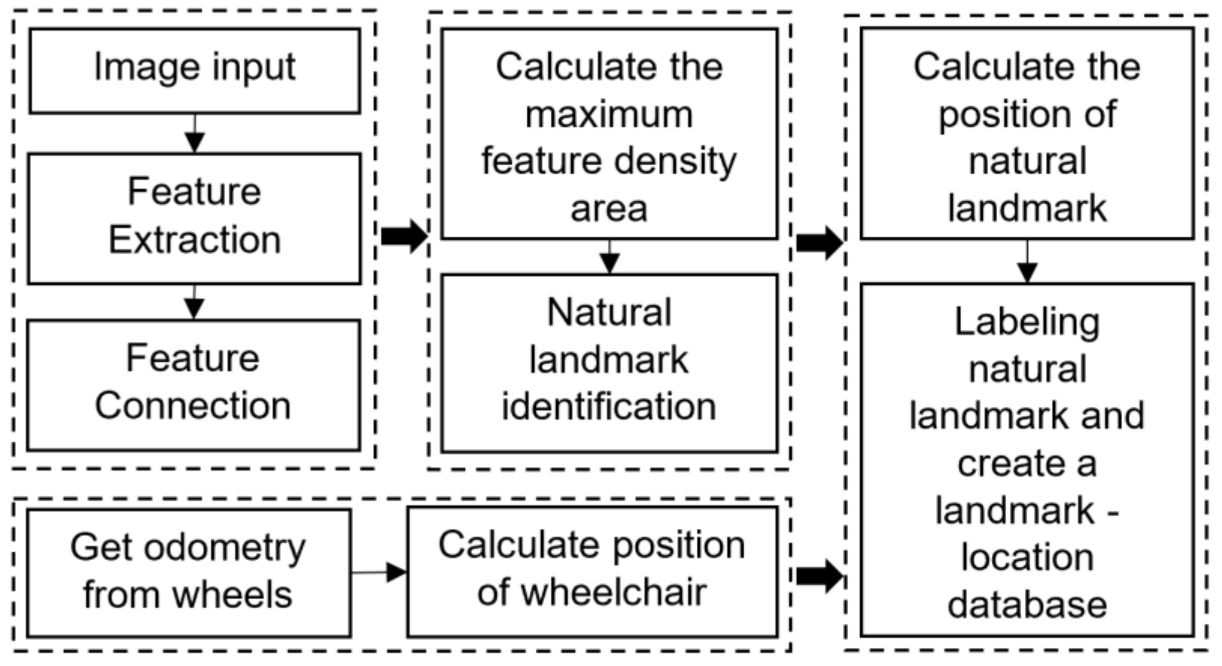
For automatic labeling of natural landmarks in an image, the feature’s detection of objects in the image can be divided into the following three groups: converting RGB image to gray image; feature detection; and searching the maximum feature density area, as shown in Figure 1. First, the features of the objects are extracted using the ORB detector [36]. Next, the dilation technique is applied to create a link between the key points of the object and then draw the bounding boxes. With the bounding boxes already obtained, the key points’ density will be calculated for these bounding boxes. Finally, the bounding boxes contain the most key points for detecting the landmark. For automatic labeling of natural landmarks, the position of landmarks is calculated based on their 3D information and the position of the wheelchair.
3.1. Extraction and Connection of Features in an Object
Feature extraction to detect landmarks in the environment plays an important role. To detect feature points, ORB detectors are applied to speed up feature extraction, because the process of detecting and determining the location of landmarks needs to be performed in real time [36]. After the feature extraction process, the retention of the key points is performed, and all other pixels without the key points are removed. Therefore, the binary image A only contains the key points (foreground) or the non-key point (background). We connect the features of the object in the image by dilating them. In particular, the dilation of a binary image A with a structuring element K as a kernel is performed, in which the centre of K is chosen to be an anchor point. Therefore, the dilated image D can be calculated as follows:
where means taking the reflection of K from its origin and shifting by Z. Hence, the dilation of A with K is a set of all displacements, Z, such that and A overlap by at least one element [54].
To better understand the idea and avoid possible confusion, we can invert an original image so that the object in white represents the key points. For connecting broken parts of an object, the dilation makes the object appear whiter and is also the dual of erosion, in which dilating foreground pixels is equivalent to eroding the background pixels. Therefore, to perform the dilation, a cross-structuring element of size K is used, described as follows:
3.2. Natural Landmark Detection
After performing the connection of the key points characteristic of the object in the image, the object is separated using the technique of finding the contours of the object. The contour refers to a curve connecting all continuous points along the boundary based on the same color or intensity. Therefore, if we find a contour in a binary image, the boundary of an object in an image is found. It is obvious that the contour is a useful tool for shape analysis and object detection. Therefore, the object should be white, and its background should be black in the binary image.
A natural landmark is defined as an object that contains many features in an image. Therefore, the detected objects with the distinctive features, which are compared to other objects in the image, are chosen to determine the object with the most features. In particular, the dilated image D with a size of r × c is processed to just contain 2 values (0,1), and the sum of the white pixels of D is determined as follows:
In similarity, the sum of the white pixels in objects of the subimage Oi with a size of hi × wi (i = 1, 2, …, n, with n being the number of objects in image D) after drawing contours is calculated as follows:
From Equations (4) and (5), the probability coefficient of key points on an object compared to the total number of key points of the original image is determined. In particular, the largest coefficient of the object defined as a natural landmark in the original image is calculated as follows:
3.3. Position of the Wheelchair in the Environment
The kinetic equation is the description of the relationship between the Oxy coordinate in the Cartesian coordinate system of the wheelchair and the velocity of two wheels, as described in Figure 2.
The wheelchair model as shown in Figure 2 can move and orient with two wheels and change its direction based on changing the velocity of the left wheel vl(t) and the right wheel vr(t). The wheelchair will move along a curvilinear trajectory around this point with the angular velocity ω(t). L is the distance between the two wheels. O(x,y) is the coordinate of the midpoint of the two wheels’ axis. θ is the angle formed by the axis of the chassis and the horizontal axis. All variables in the dynamic model of the wheelchair are considered at the instantaneous time t. In particular, the coordinates x(t), y(t) and the orientation angle θ(t) at time t are related to the angular velocity ω(t) and the velocity v(t) of the wheelchair, as in the following formula:
The coordinate of the wheelchair at time t = k + 1 is described as follows:
where dr(k + 1) and dl(k + 1) are the distances of the right and left wheels, respectively, from the time of k to (k + 1). Equation (8) shows that the coordinates of the wheelchair at time (k + 1) are determined based on the moving distances of the left and right wheels from the time of k to (k + 1) and the coordinates of the wheelchair at time k. Therefore, by reading the encoder pulses and using the kinetic equations of two wheels, we can determine the position of the wheelchair during its movement.
3.4. Automatic Labeling of Natural Landmarks
In this planning, the location of landmarks will be detected and labeled whenever the wheelchair is close to the landmarks. After detecting a natural landmark, the center of the landmark will be determined by mapping to the 3D spatial domain of the RGB-D camera, and the coordinate of the landmark center (xLM, yLM) will be determined, in which the deviation xLM of the center of the landmark from the center of the camera will be less than 0 if it is to the right of the camera and greater than 0 if the landmark is to the left of the camera. Figure 3 depicts the position of the wheelchair, and the landmark in the spatial domain, in which the wheelchair coordinates in the 2D environment are (xW, yW), and that of the landmark in the camera spatial domain are (xLM, yLM).
From Figure 3, the landmark coordinate in the 2D environment is calculated for the wheelchair coordinate as follows:
in which θ is the angle of the moving wheelchair using Equations (7) and (8). The object angle α calculated from the distance d of the detected landmark to the camera position is described as follows:
After determining the landmark position, the order number and coordinate of the landmark in the image are labeled in a format as “Name_Order_XLMG_YLMG_βLMG.JPG”.
4. Results and Discussion
In this research, a total of eight experiments were performed to demonstrate their success. For the experiments, the electric wheelchair which has an RGB-D camera and two encoders is set up to verify and validate our approach, as shown in Figure 4. We use an object in the classroom as a natural landmark in the experiments. We performed tests with different states of landmarks, including fewer landmarks, many landmarks, mobile angle, and distance to landmarks.
4.1. Natural Landmark Detection
An input image with a white wall and different objects, including information and instruction boards and switch panels, is shown in Figure 5a. In Figure 5b, the small green circles on the objects are features extracted from the input objects using the ORB detector. In addition, these features have the most distinct colors or outstanding objects compared to others. Therefore, these main features are used to detect landmarks and applied for localization and planning for mobile wheelchairs.
For the input frames of the object recognition system in real time, features need to be extracted using different methods. Table 1 shows the performance of SIFT, SURF, and ORB corner detectors in the PC environment when performing feature extraction for Figure 5a. In addition, the overall performance of the feature detector and descriptor algorithms is dependent on descriptor generation, as shown in Table 1. These SIFT, SURF, and ORB algorithms differently took time to determine the location of the initial key points, in which the feature extraction rate of one key point using the SIFT and SURF algorithms is set up to be nearly similar to and slower than ORB.
For processing dilation of images, the 3 × 3 kernel K with the common structuring element was applied if a kernel with the structure of more or fewer elements often affects dilation results. Figure 6 shows the connection of the main features of the objects, as shown in Figure 5, where the dilation of the main features is performed in different iterations. With different repetitions, the main features of the object will be dilated and then show connectivity problems, such as main features at discrete or overlapping positions. In particular, with one repeat, Figure 6a shows the discrete main features of the object, while with the number of the different increasing repetitions, the overlap of the main features will appear, as shown in Figure 6b–d. As a result of the repetition of feature point dilations, the number of features found based on the lengths of the contours also changes. In particular, Figure 6a,b show that four bounding boxes are detected and assigned symbols (from #1 to #4), while only three bounding boxes are detected for a feature frame as shown in Figure 6c,d (from #1 to #3). It can be seen that when the number of iterations is one, the objects are incorrectly defined and incomplete. In particular, the algorithm could not detect the switch panels, while the dark blue bulletin board could recognize two objects. In the case of a large number of iterations (10 or 15 iterations), the number of detected objects is still wrong, in which the switch panels and the indicator panels are overlapped to be an object. Therefore, with five iterations, the objects in the image are exactly detected, as shown in Figure 6. It means that the five iterations are most suitable for detecting objects, and it is a basis for selecting a typical landmark based on feature density.
In this article, during wheelchair movement, images with natural objects were captured at different distances from an RGB-D camera system. In Figure 7, an environmental image with five objects and the wall was captured at the distance of 2 m from the camera to the wall, in which the five objects show different feature densities. In particular, the object with a white instruction bulletin board has the largest density of using Equation (6), so the recognition system will choose this instruction bulletin board to be the landmark. Figure 8 shows that the system recognizes the image with two objects at a distance of 1 m from the camera to the wall. Figure 8c shows that the second object is chosen to be the landmark corresponding to the largest density of compared to the remaining object.
Another experiment for testing the accuracy of the detection algorithm of natural landmarks was worked out by measuring the Intersection over Union (IoU) between two boxes, in which one box contains real objects and another one containing a landmark is selected using the proposed algorithm [55]. Moreover, the larger the overlap, the larger the IoU. This indicates that the ability to select the object as a landmark is really correct. Therefore, the predictive results could be good if the IoU exceeds 0.5. Assuming that box 1 is represented by [x1, y1, x2, y2] and box 2 is [x3, y3, x4, y4], as shown in Figure 9a, the IoU is calculated as shown in Figure 9b.
Table 2 shows the IoU values in case of similarly performing at five different distances and 10 times. The average IoU value of 10 times of experiments with the five different distances is greater than 0.5, in which the experiments to detect landmarks at distances of 1 m and 2 m have the same IoU value, which is the largest with more than 0.86. In particular, in 10 experiments for each distance of 1 m and 2 m, the IoU value was between 0.8 and 0.92, while the IoU value was between 0.53 and 0.72 at the distance of 3 m. For the 4 m and 5 m distances, the average IoU values were low with 0.56 and 0.52, respectively. This means that, at different distances, the algorithm still provides good detection results, but with close distances less than 2 m, the detection results have the highest accuracy.
Table 3 describes the experiment for detecting landmarks with different lighting conditions and at different distances. From this table, it can be seen that, at the distance of 1 m and 2 m, the IoU value is greater than 0.8. This means that the recognition results are good, and the features extracted using the ORB detector have good invariance to changes in illuminance. In addition, when the distance from the landmark to the camera is more than 2 m, the IoU values are less than 0.8 and are reduced with light intensity. Figure 10 depicts two natural landmarks detected in the experimental environment described in Table 3.
Experiments with different angles between the camera position and objects, such as the right wall of the laboratory, were performed as shown in Figure 11, Figure 12 and Figure 13. In particular, these object images were taken at the angles of 0°, 35°, and 45°, respectively. The results show that the proposed algorithm correctly recognizes the same object with different shooting angles, which will be selected as a landmark. In addition, Figure 11d, Figure 12d, and Figure 13d show that the bounding box in which the proposed algorithm predicts the landmark (red rectangle) overlaps most of the ground-truth bounding box, called the actual landmark (green rectangle). The IoU value in all three cases is greater than 0.8, indicating that the accuracy is very high.
The results of recognizing natural landmarks in indoor environments are shown in Figure 14. In particular, images from the left to right and the recognized objects in each pair of these images were contoured by the blue-color rectangles, and the most prominent objects were chosen to be the landmarks marked by the red-color contours. Moreover, the average time for processing each step is shown in Table 4, in which it takes the most time for the calculation to determine a landmark by calculating the feature density of the object. With an average total time of 41.66 ms for recognizing a landmark, the recognition system may be considered the fast processing speed with real time.
In the indoor environment, the prominent landmarks can be chosen using the proposed method and various landmarks of the doors, stairs [13], and the areas with uniform color were recognized [26]. Therefore, the motioned wheelchair can easily recognize these landmarks in complex natural environments. Our approach and studies [13,26] both aim to perform online without pretraining steps when detecting landmarks. Specifically, the study [13] has proposed a robust method for detecting natural landmarks using 3D point cloud data with over 90% accuracy when recognizing doors and stairs. In addition, a fast vision-based object segmentation technique has been proposed by research [26] to detect natural landmarks for mobile robots in indoor environments. This method can detect walls, doors, floors, and ceilings by finding straight lines and then generating convex polygons, with the whole process of the method losing less than 80 ms. The difference between these studies is that our method mainly focuses on detecting objects in the natural environment with a variety of landmarks. Moreover, compared with the object detection methods in the articles [42,43], our proposed method is based on the density of feature points of the regions in the proposed objects, so it shows fewer objects in the image. As a result, the processing time of object detection in the image for selection and collection of landmarks will be faster and has the potential for real-time applications.
4.2. Results of Locating Landmarks
In this article, we performed distance measurements from the camera’s center to landmarks using the RealSense D435 camera and then compared them with the true distances of those landmarks in the lab environment. Figure 15 represents the relative error between the average measuring distance and the distances of the actual landmarks, in which each position is measured 100 times. It is obvious that the relative distance error has a change of 0.01% to 0.07%. When the detection algorithm makes a landmark prediction with a low IoU value, the average depth value may be out of the object. Therefore, this is true for small objects, and they are noted at the peaks of 3.5 m and 5.0 m, as shown in Figure 15.
The next experiment is that the position error of the wheelchair in the 2D space is checked using the encoder data. In this experiment, the wheelchair was moved along a reference line (red line), and then the position data of the wheelchair were recorded (blue line), as shown in Figure 16. As shown in Figure 16a, the wheelchair moved to the position x = 2 m, y = 5 m in the 2D space following a pre-established line. Assuming that the initial coordinates of the wheelchair are x = 0, y = 0, as shown in Figure 16b, the wheelchair moved to the position x = 2 m, y = 2 m. In Figure 16c, the wheelchair moved to the position x = 2 m, y = 10 m. Therefore, the trajectory of the wheelchair moving to the position x = 2 m, y = 5 m with the perpendicular corner points is described in Figure 16d.
The position error of the wheelchair in three experiments (Figure 16a–c) is shown in Table 5. In particular, the calculated wheelchair position has an error of less than or equal to 4.0 cm on the x-axis and less than or equal to 2.0 cm on the y-axis. This error of the wheelchair is due to the change in directions during movement, causing the position error due to the inertia of the wheelchair. Figure 16d depicts the real path (blue line) and reference path (red line) of the wheelchair. When moving from A to B and B to C, the average position error of the wheelchair is less than 1 cm. After that, when moving from C to D, the wheelchair position has an error of about 4 cm along the x-axis. Finally, at the end point E, the actual position of the wheelchair has an error of 1.5 cm from the ground-truth position on the x-axis and 2.0 cm on the y-axis.
Table 6 describes the results of determining landmark positions with different experiments. In particular, the wheelchair collected landmark positions during movement to other places. Therefore, the landmark positions are calculated based on the proposed method, and then the computed positions are compared with their real positions in the environment. From Table 6, it can be seen that with the distance from the camera to the landmark object less than 200 cm, the landmark position has an error of less than 3.0 cm on the x-axis and less than 2.0 cm on the y-axis. If the distance from the camera to the landmark is larger than 200 cm, the error can increase, particularly about 15.0 cm on the x-axis and 7.0 cm on the y-axis. This can mean that it should collect and label landmarks with a distance of less than 200 cm in the environment so that the collected landmarks achieve high accuracy.
The results from the experiments have shown that the proposed automatic labeling system for landmarks in the environment may be applied to real wheelchairs or robots in indoor environments. This study contributed to an automatic location labeling tool for landmarks in indoor environments, which may be applied to different fields. Table 7 lists the research works on automatic labeling of objects in images. In particular, one study [32] proposed a new automatic AR-based annotation tool for detecting and labeling prominent objects such as tables, chairs, and low ceilings for indoor navigation applications. This study employed the YOLOv3 algorithm for object detection, longitude and latitude positioning, and object labeling in the database. Different from this study, our study applied the method of detecting natural landmarks in the indoor environment based on their maximum feature density. With our approach, it required a fast processing time without pretraining. Moreover, using the object position according to longitude and latitude, as in [32], is suitable for a large environment. However, with a small environment and higher accuracy requirement, our proposed method for locating landmarks in 2D space would be more appropriate.
In relation to previous studies [33,34,35], our study has shown the process of on automatically performing object collection and labeling. The time to finish this process is substantially reduced compared to the manual labeling process. With the relation in previous studies, the study [33] presented a new approach with the automatic process of collecting and annotating data on a six-degrees-of-freedom (6-DoF) posture of objects in the image. With this approach, the process reduced execution time; particularly, it only takes 40 s instead of about 4.5 h. This is essential for many applications in the existing systems, such as robotics, autonomous driving and vision-based navigation, artificial intelligence, and autonomous driving for unmanned aircraft systems (UAS). In [34], the research indicates that previous methods used manual annotation and spent much time collecting eye-tracking data, so this research proposed a system combined with an object detection algorithm using Mask R-based deep CNN and frame-by-frame gaze coordinates measured by eye-tracking equipment. This research allowed them to detect and annotate eye activities without any manual requirements. In addition, a fast vision-based object segmentation technique [26] was applied for natural landmark detection on the indoor mobile robot method, and the whole execution time of the object detection is about 75 ms, compared to 41.66 ms using our proposed method.
Data collection from automated devices may be inaccurate depending on the nature of the application, sensor type, complexity of the data, and the process of evaluating the information collected [56]. This raises an ethical issue of the machine giving incorrect information that could lead to serious action, such as a wheelchair going astray or a collision. Automated information sharing and collection in wheelchair systems can be useful in some situations, e.g., a hospital or nursing home consisting of multiple autonomous wheelchairs sharing the same database will save operating costs. However, if a database of landmarks is collected within an individual residence, this raises ethical concerns that the data collection system captures more detail than information is provided. In particular, this video intrusion could cause a significant breach of privacy and risk exposing users’ lives through viewing their private spaces and personal behaviors. Therefore, the ethical and social implications of using camera systems for wheelchair navigation and motion planning need to be given special attention when applied to practical applications.
5. Conclusions
This paper has proposed a method to automatically detect natural landmarks labeled for defining the location in the lab environment. In particular, we used the density of feature points extracted from the ORB to detect the natural landmarks. The depth of the RGB-D camera and encoders on two wheels showed the position information. In the experiments, the detected landmarks achieve high accuracy by calculating the IoU values. These IoU values are over 0.8 at a distance of less than 2 m from the camera to the landmark, gaining the best performance. The defined positions from this system have a slight error compared to their actual places. Besides, the system’s processing speed is suitable for real-time applications. In the field of computer vision, pattern recognition and machine learning can recognize objects in images or videos such as faces, objects, people, or animals with high accuracy and fast processing time [57]. Pattern recognition and machine learning models learn from data and therefore need to be fed a complete database of objects. This is different from our proposed method, which does not require pretraining for the recognition. The obtained results demonstrate the effectiveness of the proposed method. Therefore, the automatic labeling of natural landmarks is a potential solution for mobile wheelchairs or robots in complex environments.
Author Contributions
Conceptualization, B.-V.N., T.-H.N. and C.C.V.; Methodology, B.-V.N., T.-H.N. and C.C.V.; Software, B.-V.N. and T.-H.N.; Validation, B.-V.N., T.-H.N. and C.C.V.; Formal analysis, B.-V.N. and T.-H.N.; Investigation, B.-V.N. and T.-H.N.; Resources, B.-V.N. and T.-H.N.; Data curation, B.-V.N. and T.-H.N.; Writing—original draft, B.-V.N., T.-H.N. and C.C.V.; Writing—review & editing, B.-V.N., T.-H.N. and C.C.V.; Visualization, B.-V.N. and T.-H.N.; Supervision, B.-V.N. and T.-H.N.; Project administration, B.-V.N. and T.-H.N.; Funding acquisition, B.-V.N., T.-H.N. and C.C.V. All authors have read and agreed to the published version of the manuscript.
Funding
This research received no external funding.
Data Availability Statement
The datasets generated and/or analyzed during the current study are available from the corresponding author on reasonable request.
Acknowledgments
We would like to thank the Ho Chi Minh City University of Technology and Education (HCMUTE), Vietnam.
Conflicts of Interest
The authors declare no conflict of interest.
References
- Zhang, J.; Singh, S. Visual-lidar odometry and mapping: Low-drift, robust, and fast. In Proceedings of the 2015 IEEE International Conference on Robotics and Automation (ICRA), Seattle, WA, USA, 26–30 May 2015; pp. 2174–2181. [Google Scholar]
- Hai, T.; Nguyen, V.B.N.; Hai, T. Quach. Optimization of Transformation Matrix for 3D Cloud Mapping Using Sensor Fusion. Am. J. Signal Process. 2018, 8, 9–19. [Google Scholar] [CrossRef]
- Liu, T.; Wang, Y.; Niu, X.; Chang, L.; Zhang, T.; Liu, J. LiDAR Odometry by Deep Learning-Based Feature Points with Two-Step Pose Estimation. Remote Sens. 2022, 14, 17. [Google Scholar] [CrossRef]
- Kuo, B.-W.; Chang, H.-H.; Chen, Y.-C.; Huang, S.-Y. A Light-and-Fast SLAM Algorithm for Robots in Indoor Environments Using Line Segment Map. J. Robot. 2011, 2011, 257852. [Google Scholar] [CrossRef] [Green Version]
- Beyer, L.; Hermans, A.; Leibe, B. DROW: Real-Time Deep Learning-Based Wheelchair Detection in 2-D Range Data. IEEE Robot. Autom. Lett. 2017, 2, 585–592. [Google Scholar] [CrossRef] [Green Version]
- Alatise, M.B.; Hancke, G.P. Pose Estimation of a Mobile Robot Based on Fusion of IMU Data and Vision Data Using an Extended Kalman Filter. Sensors 2017, 17, 22. [Google Scholar] [CrossRef] [Green Version]
- McConville, A.; Bose, L.; Clarke, R.; Mayol-Cuevas, W.; Chen, J.; Greatwood, C.; Carey, S.; Dudek, P.; Richardson, T. Visual Odometry Using Pixel Processor Arrays for Unmanned Aerial Systems in GPS Denied Environments. Front. Robot. AI 2020, 7, 126. [Google Scholar] [CrossRef]
- Yang, H.; Bao, X.; Zhang, S.; Wang, X. A Multi-Robot Formation Platform based on an Indoor Global Positioning System. Appl. Sci. 2019, 9, 16. [Google Scholar] [CrossRef] [Green Version]
- Marques, T.P.; Hamano, F. Autonomous robot for mapping using ultrasonic sensors. In Proceedings of the 2017 IEEE Green Energy and Smart Systems Conference (IGESSC), Long Beach, CA, USA, 6–7 November 2017; pp. 1–6. [Google Scholar]
- Tsotsos, K.; Chiuso, A.; Soatto, S. Robust inference for visual-inertial sensor fusion. In Proceedings of the 2015 IEEE International Conference on Robotics and Automation (ICRA), Seattle, WA, USA, 26–30 May 2015; pp. 5203–5210. [Google Scholar]
- Fang, W.; Zhang, J.G.; Song, H.Y. Global and Local Path Planning on Robotic Wheelchair Based on Multi-Sensor Information Fusion. Adv. Mater. Res. 2013, 655–657, 1145–1148. [Google Scholar] [CrossRef]
- Li, A.; Ruan, X.; Huang, J.; Zhu, X.; Wang, F. Review of vision-based Simultaneous Localization and Mapping. In Proceedings of the 2019 IEEE 3rd Information Technology, Networking, Electronic and Automation Control Conference (ITNEC), Chengdu, China, 15–17 March 2019; pp. 117–123. [Google Scholar]
- Souto, L.A.V.; Castro, A.; Gonçalves, L.M.G.; Nascimento, T.P. Stairs and Doors Recognition as Natural Landmarks Based on Clouds of 3D Edge-Points from RGB-D Sensors for Mobile Robot Localization. Sensors 2017, 17, 16. [Google Scholar] [CrossRef] [Green Version]
- Vidal, J.; Lin, C. Simple and robust localization system using ceiling landmarks and infrared light. In Proceedings of the 2016 12th IEEE International Conference on Control and Automation (ICCA), Kathmandu, Nepal, 1–3 June 2016; pp. 583–587. [Google Scholar]
- Kartashov, D.; Huletski, A.; Krinkin, K. Fast artificial landmark detection for indoor mobile robots. In Proceedings of the 2015 Federated Conference on Computer Science and Information Systems (FedCSIS), Lodz, Poland, 13–16 September 2015; pp. 209–214. [Google Scholar]
- Xu, Y.; Liu, C.; Gu, J.; Zhang, J.; Hua, L.; Dai, Q.; Gu, H.; Xu, Z.; Xu, Y.; Gu, J.; et al. Design and recognition of monocular visual artificial landmark based on arc angle information coding. In Proceedings of the 2018 33rd Youth Academic Annual Conference of Chinese Association of Automation (YAC), Nanjing, China, 18–20 May 2018; pp. 722–727. [Google Scholar]
- Epstein, R.A.; Vass, L.K. Neural systems for landmark-based wayfinding in humans. Philos. Trans. R. Soc. Lond B Biol. Sci. 2014, 369, 7. [Google Scholar] [CrossRef]
- Viet, N.B.; Hai, N.T.; Hung, N.V. Tracking landmarks for control of an electric wheelchair using a stereoscopic camera system. In Proceedings of the 2013 International Conference on Advanced Technologies for Communications (ATC 2013), Ho Chi Minh, Vietnam, 16–18 October 2013; pp. 339–344. [Google Scholar]
- Yu, T.; Shen, Y. Asymptotic Performance Analysis for Landmark Learning in Indoor Localization. IEEE Commun. Lett. 2018, 22, 740–743. [Google Scholar] [CrossRef]
- Zhong, X.; Zhou, Y.; Liu, H. Design and recognition of artificial landmarks for reliable indoor self-localization of mobile robots. Int. J. Adv. Robot. Syst. 2017, 14, 1729881417693489. [Google Scholar] [CrossRef] [Green Version]
- Lan, G.; Wang, J.; Chen, W. An improved indoor localization system for mobile robots based on landmarks on the ceiling. In Proceedings of the 2016 IEEE International Conference on Robotics and Biomimetics (ROBIO), Qingdao, China, 3–7 December 2016; pp. 1395–1400. [Google Scholar]
- Shih, C.-L.; Ku, Y.-T. Image-Based Mobile Robot Guidance System by Using Artificial Ceiling Landmarks. J. Comput. Commun. 2016, 4, 1–14. [Google Scholar] [CrossRef]
- Lecrosnier, L.; Khemmar, R.; Ragot, N.; Decoux, B.; Rossi, R.; Kefi, N.; Ertaud, J.-Y. Deep Learning-Based Object Detection, Localisation and Tracking for Smart Wheelchair Healthcare Mobility. Int. J. Environ. Res. Public Health 2021, 18, 91. [Google Scholar] [CrossRef]
- Hong, W.; Xia, H.; An, X.; Liu, X. Natural landmarks based localization algorithm for indoor robot with binocular vision. In Proceedings of the 2017 29th Chinese Control and Decision Conference (CCDC), Chongqing, China, 28–30 May 2017; pp. 3313–3318. [Google Scholar]
- Zhang, X.; Zhu, S.; Wang, Z.; Li, Y. Hybrid visual natural landmark–based localization for indoor mobile robots. Int. J. Adv. Robot. Syst. 2018, 15, 1729881418810143. [Google Scholar] [CrossRef] [Green Version]
- Chai, X.; Wen, F.; Yuan, K. Fast vision-based object segmentation for natural landmark detection on Indoor Mobile Robot. In Proceedings of the 2011 IEEE International Conference on Mechatronics and Automation, Beijing, China, 7–10 August 2011; pp. 2232–2237. [Google Scholar]
- Bayar, B.; Stamm, M.C. Design Principles of Convolutional Neural Networks for Multimedia Forensics. In Proceedings of the Media Watermarking, Security, and Forensics, Burlingame, CA, USA, 29 January–2 February 2017. [Google Scholar]
- Ren, S.; He, K.; Girshick, R.; Sun, J. Faster R-CNN: Towards real-time object detection with region proposal networks. In Proceedings of the 28th International Conference on Neural Information Processing Systems—Volume 1, Montreal, QC, Canada, 7–12 December 2015; pp. 91–99. [Google Scholar]
- Nilwong, S.; Hossain, D.; Kaneko, S.-I.; Capi, G. Deep Learning-Based Landmark Detection for Mobile Robot Outdoor Localization. Machines 2019, 7, 25. [Google Scholar] [CrossRef] [Green Version]
- Wang, R.; You, Y.; Zhang, Y.; Zhou, W.; Liu, J. Ship detection in foggy remote sensing image via scene classification R-CNN. In Proceedings of the 2018 International Conference on Network Infrastructure and Digital Content (IC-NIDC), Guiyang, China, 22–24 August 2018; pp. 81–85. [Google Scholar]
- Jiang, S.; Kong, Y.; Fu, Y. Deep Geo-Constrained Auto-Encoder for Non-Landmark GPS Estimation. IEEE Trans. Big Data 2019, 5, 120–133. [Google Scholar] [CrossRef]
- Du, P.; Bulusu, N. An automated AR-based annotation tool for indoor navigation for visually impaired people. In Proceedings of the 23rd International ACM SIGACCESS Conference on Computers and Accessibility, Virtual Event, 18–22 October 2021; pp. 1–4. [Google Scholar]
- Apud Baca, J.G.; Jantos, T.; Theuermann, M.; Hamdad, M.A.; Steinbrener, J.; Weiss, S.; Almer, A.; Perko, R. Automated Data Annotation for 6-DoF AI-Based Navigation Algorithm Development. J. Imaging 2021, 7, 236. [Google Scholar] [CrossRef]
- Deane, O.; Toth, E.; Yeo, S.-H. Deep-SAGA: A deep-learning-based system for automatic gaze annotation from eye-tracking data. Behav. Res. Methods 2022, 55, 1372–1391. [Google Scholar] [CrossRef]
- García-Aguilar, I.; García-González, J.; Luque-Baena, R.M.; López-Rubio, E. Automated labeling of training data for improved object detection in traffic videos by fine-tuned deep convolutional neural networks. Pattern Recognit. Lett. 2023, 167, 45–52. [Google Scholar] [CrossRef]
- Rublee, E.; Rabaud, V.; Konolige, K.; Bradski, G. ORB: An efficient alternative to SIFT or SURF. In Proceedings of the 2011 International Conference on Computer Vision, Barcelona, Spain, 6–13 November 2011; pp. 2564–2571. [Google Scholar]
- Mur-Artal, R.; Montiel, J.M.M.; Tardós, J.D. ORB-SLAM: A Versatile and Accurate Monocular SLAM System. IEEE Trans. Robot. 2015, 31, 1147–1163. [Google Scholar] [CrossRef] [Green Version]
- Lampert, C.H.; Blaschko, M.B.; Hofmann, T. Beyond sliding windows: Object localization by efficient subwindow search. In Proceedings of the 2008 IEEE Conference on Computer Vision and Pattern Recognition, Anchorage, Alaska, 23–28 June 2008; pp. 1–8. [Google Scholar]
- Manen, S.; Guillaumin, M.; Gool, L.V. Prime Object Proposals with Randomized Prim’s Algorithm. In Proceedings of the 2013 IEEE International Conference on Computer Vision, Sydney, Australia, 1–8 December 2013; pp. 2536–2543. [Google Scholar]
- Carreira, J.; Sminchisescu, C. CPMC: Automatic Object Segmentation Using Constrained Parametric Min-Cuts. IEEE Trans. Pattern Anal. Mach. Intell. 2012, 34, 1312–1328. [Google Scholar] [CrossRef] [PubMed]
- Alexe, B.; Deselaers, T.; Ferrari, V. Measuring the Objectness of Image Windows. IEEE Trans. Pattern Anal. Mach. Intell. 2012, 34, 2189–2202. [Google Scholar] [CrossRef] [Green Version]
- Endres, I.; Hoiem, D. Category-Independent Object Proposals with Diverse Ranking. IEEE Trans. Pattern Anal. Mach. Intell. 2014, 36, 222–234. [Google Scholar] [CrossRef]
- Uijlings, J.R.R.; van de Sande, K.E.A.; Gevers, T.; Smeulders, A.W.M. Selective Search for Object Recognition. Int. J. Comput. Vis. 2013, 104, 154–171. [Google Scholar] [CrossRef] [Green Version]
- Felzenszwalb, P.F.; Huttenlocher, D.P. Efficient Graph-Based Image Segmentation. Int. J. Comput. Vis. 2004, 59, 167–181. [Google Scholar] [CrossRef]
- Jiang, Y.; Xu, Y.; Liu, Y. Performance evaluation of feature detection and matching in stereo visual odometry. Neurocomputing 2013, 120, 380–390. [Google Scholar] [CrossRef]
- Lyu, W.; Zhou, Z.; Chen, L.; Zhou, Y. A survey on image and video stitching. Virtual Real. Intell. Hardw. 2019, 1, 55–83. [Google Scholar] [CrossRef]
- Xie, H.; Yao, H.; Zhou, S.; Zhang, S.; Tong, X.; Sun, W. Toward 3D object reconstruction from stereo images. Neurocomputing 2021, 463, 444–453. [Google Scholar] [CrossRef]
- Elliott, J.; Khandare, S.; Butt, A.A.; Smallcomb, M.; Vidt, M.E.; Simon, J.C. Automated Tissue Strain Calculations Using Harris Corner Detection. Ann. Biomed. Eng. 2022, 50, 564–574. [Google Scholar] [CrossRef]
- Rosten, E.; Drummond, T. Machine Learning for High-Speed Corner Detection. In Proceedings of the Computer Vision—ECCV 2006, Berlin, Heidelberg, 7–13 May 2006; pp. 430–443. [Google Scholar]
- Lowe, D.G. Distinctive Image Features from Scale-Invariant Keypoints. Int. J. Comput. Vis. 2004, 60, 91–110. [Google Scholar] [CrossRef]
- Bay, H.; Tuytelaars, T.; Van Gool, L. SURF: Speeded Up Robust Features. In Proceedings of the Computer Vision—ECCV 2006, Graz, Austria, 7–13 May 2006; pp. 404–417. [Google Scholar]
- Liu, Y.; Zhang, H.; Guo, H.; Xiong, N.N. A FAST-BRISK Feature Detector with Depth Information. Sensors 2018, 18, 3908. [Google Scholar] [CrossRef] [PubMed] [Green Version]
- Gueguen, L.; Pesaresi, M. Multi scale Harris corner detector based on Differential Morphological Decomposition. Pattern Recognit. Lett. 2011, 32, 1714–1719. [Google Scholar] [CrossRef]
- Richard, E.; Woods, P.A.W. Digital Image Processing, 4th ed.; Pearson India: Noida, India, 2019. [Google Scholar]
- Salau, J.; Krieter, J. Instance Segmentation with Mask R-CNN Applied to Loose-Housed Dairy Cows in a Multi-Camera Setting. Animals 2020, 10, 2402. [Google Scholar] [CrossRef] [PubMed]
- Stojmenovic, I. Fog computing: A cloud to the ground support for smart things and machine-to-machine networks. In Proceedings of the 2014 Australasian Telecommunication Networks and Applications Conference (ATNAC), Melbourne, Australia, 26–28 November 2014; pp. 117–122. [Google Scholar]
- Bishop, C.M. Pattern Recognition and Machine Learning; Springer: New York, NY, USA, 2006. [Google Scholar]
Figure 1.
Structure of the automatic landmark map generation procedure.

Figure 2.
Dynamic model of the wheelchair with four wheels.

Figure 3.
Estimation of the predicted landmark position.

Figure 4.
Wheelchair with the RGB-D camera, encoder, and PC.

Figure 5.
Objects with corner feature: (a) RGB image; (b) image with key points.

Figure 6.
Object contours and feature frames: (a) one iteration; (b) five iterations; (c) ten iterations; (d) fifteen iterations.
Figure 6.
Object contours and feature frames: (a) one iteration; (b) five iterations; (c) ten iterations; (d) fifteen iterations.

Figure 7.
Representation of the process for the landmark recognition in the natural lab environment at the distance of 2 m from the camera to objects: (a) image with key points; (b) dilated image; (c) feature frames image; (d) objects image; (e) landmark image.
Figure 7.
Representation of the process for the landmark recognition in the natural lab environment at the distance of 2 m from the camera to objects: (a) image with key points; (b) dilated image; (c) feature frames image; (d) objects image; (e) landmark image.

Figure 8.
Representation of the process for the landmark recognition in the natural lab environment at the distance of 1 m from the camera to objects: (a) image with key points; (b) dilated image; (c) feature frames image; (d) objects image; (e) landmark image.
Figure 8.
Representation of the process for the landmark recognition in the natural lab environment at the distance of 1 m from the camera to objects: (a) image with key points; (b) dilated image; (c) feature frames image; (d) objects image; (e) landmark image.

Figure 9.
IoU for bounding boxes: (a) intersection of two boxes; (b) representation of the formula to calculate IoU.
Figure 9.
IoU for bounding boxes: (a) intersection of two boxes; (b) representation of the formula to calculate IoU.

Figure 10.
Recognition of the natural landmark in the lab environment with different lighting conditions: (a) images with landmark 1; (b) images with landmark 2.
Figure 10.
Recognition of the natural landmark in the lab environment with different lighting conditions: (a) images with landmark 1; (b) images with landmark 2.


Figure 11.
Recognition of the natural landmark in the lab environment at the angle of 0°: (a) image with main points; (b) objects image; (c) landmark image; (d) ground-truth bounding box and landmark bounding box image.
Figure 11.
Recognition of the natural landmark in the lab environment at the angle of 0°: (a) image with main points; (b) objects image; (c) landmark image; (d) ground-truth bounding box and landmark bounding box image.

Figure 12.
Recognition of the natural landmark in the lab environment at the angle of 45°: (a) image with main points; (b) objects image; (c) landmark image; (d) ground-truth bounding box and landmark bounding box image.
Figure 12.
Recognition of the natural landmark in the lab environment at the angle of 45°: (a) image with main points; (b) objects image; (c) landmark image; (d) ground-truth bounding box and landmark bounding box image.

Figure 13.
Recognition of the natural landmark in the lab environment at the angle of 30°: (a) image with main points; (b) objects image; (c) landmark image; (d) ground-truth bounding box and landmark bounding box image.
Figure 13.
Recognition of the natural landmark in the lab environment at the angle of 30°: (a) image with main points; (b) objects image; (c) landmark image; (d) ground-truth bounding box and landmark bounding box image.

Figure 14.
Natural landmarks detected from different areas: (a) image frames on the wall in the corridor; (b) recognized landmark on the wall in the corridor; (c) image frames on another wall in the corridor; (d) recognized landmark on another wall in the corridor; (e) image frames on the wall of the lab room; (f) recognized landmark on the wall of the lab room; (g) image frames on another wall of the lab room; (h) recognized landmark on another wall of the lab room.

Figure 15.
The relative distance of the detected landmarks measurement error.

Figure 16.
Representation of the wheelchair movement trajectory to the preset positions: (a) Experiment-1; (b) Experiment-2; (c) Experiment-3; (d) Experiment-4.
Figure 16.
Representation of the wheelchair movement trajectory to the preset positions: (a) Experiment-1; (b) Experiment-2; (c) Experiment-3; (d) Experiment-4.


Table 1.
Real-time feature extraction results using different detectors.
| Detector | Time Per Frame (ms) | Time Per Key Point (ms) | Number of Key Points in Frame |
|---|---|---|---|
| SIFT [50] | 31.08 | 0.07 | 426 |
| SURF [51] | 17.55 | 0.08 | 230 |
| ORB [36] | 3.74 | 0.002 | 1850 |
Table 2.
IoU with different distances.
| No. | Distance 1 m | Distance 2 m | Distance 3 m | Distance 4 m | Distance 5 m |
|---|---|---|---|---|---|
| 1 | 0.86 | 0.83 | 0.72 | 0.56 | 0.68 |
| 2 | 0.9 | 0.92 | 0.57 | 0.61 | 0.5 |
| 3 | 0.91 | 0.83 | 0.53 | 0.55 | 0.48 |
| 4 | 0.86 | 0.85 | 0.56 | 0.54 | 0.47 |
| 5 | 0.89 | 0.91 | 0.55 | 0.63 | 0.6 |
| 6 | 0.8 | 0.9 | 0.55 | 0.58 | 0.28 |
| 7 | 0.8 | 0.8 | 0.57 | 0.49 | 0.56 |
| 8 | 0.88 | 0.83 | 0.55 | 0.47 | 0.48 |
| 9 | 0.86 | 0.86 | 0.55 | 0.55 | 0.6 |
| 10 | 0.8 | 0.85 | 0.63 | 0.62 | 0.56 |
| Average | 0.86 | 0.86 | 0.58 | 0.56 | 0.52 |
Table 3.
IoU with different lighting conditions.
| Distance | Standard Lighting | Low Lighting | Lowest Lighting | |||
|---|---|---|---|---|---|---|
| Landmark 1 | Landmark 2 | Landmark 1 | Landmark 2 | Landmark 1 | Landmark 2 | |
| 1 m | 0.84 | 0.86 | 0.82 | 0.85 | 0.84 | 0.86 |
| 2 m | 0.84 | 0.82 | 0.90 | 0.80 | 0.90 | 0.82 |
| 3 m | 0.77 | 0.59 | 0.70 | 0.50 | 0.51 | 0.45 |
Table 4.
Processing time for landmark recognition of the proposed method.
| Stages of Implementation | Figure 14a | Figure 14c | Figure 14e | Figure 14g |
|---|---|---|---|---|
| Feature extraction [ms] | 2.90 | 3.77 | 2.89 | 4.77 |
| Object detection and landmark recognition [ms] | 37.10 | 37.93 | 36.12 | 41.16 |
| Total [ms] | 40.00 | 41.70 | 39.01 | 45.93 |
Table 5.
Evaluation of the position error of the wheelchair—Unit: cm.
| No. | Ground Truth | Actual Position | |Δx| | |Δy| |
|---|---|---|---|---|
| 1 | (200.0, 500.0) | (203.0, 502.0) | 3.0 | 2.0 |
| 2 | (200.0, 200.0) | (204.0, 201.0) | 4.0 | 1.0 |
| 3 | (200.0, 100.0) | (201.0, 99.0) | 1.0 | 1.0 |
Table 6.
Results of locating landmarks based on the wheelchair position—Unit: cm.
| Wheelchair Position (xw, yw, θw) | Distance to Landmark d | Position of Actual Landmark | Landmark Position Calculated Using the Proposed Method | |Δx| | |Δy| |
|---|---|---|---|---|---|
| (30.0, 30.0, 90) | 96.8 | (60.6, 121.1) | (63.1, 120.9) | 2.5 | 0.2 |
| (30.0, 30.0, 45) | 85.9 | (90.7, 90.7) | (92.2, 89.2) | 1.5 | 1.5 |
| (40.0, 40.0, 60) | 112.7 | (120.0, 120.0) | (119.5, 119.9) | 0.5 | 0.1 |
| (40.0, 40.0, 30) | 111.0 | (120.0, 120.0) | (128.6, 106.9) | 8.6 | 13.1 |
| (80.0, 40.0, 120) | 89.1 | (40.0, 120.0) | (38.7, 119.0) | 1.3 | 1.0 |
| (60.5, 60.5, 90) | 94.4 | (85.0, 151.4) | (82.4, 152.3) | 2.6 | 0.9 |
| (324.8, 116.6, 45) | 207.0 | (495.2, 124.2) | (511.1, 206.9) | 15.9 | 7.3 |
Table 7.
Automatic labeling system for objects overview.
| Works | Objects | Object Detection Technique | Dataset for Pretraining | Processing Time | Description of the Collected Dataset |
|---|---|---|---|---|---|
| [26] | Doors, walls, ceilings, and floor | Object segmentation | Do not use | 75 ms | Landmarks in an indoor environment |
| [32] | Tables, chairs, and low ceilings | YOLOv3 | Millar Library | - | Objects with their longitude and latitude |
| [33] | Toys | CNNs | MS COCO | 40 s | A six-degrees-of-freedom (6-DoF) posture of objects |
| [34] | Mobile eye-tracking data | Mask R-CNN | MS COCO | 1500 ms | Gaze coordinates |
| [35] | Vehicles | EfficientDet D4 | COCO | - | Objects with their coordinates in image |
| Proposed Method | Natural landmark | Maximum feature density | Do not use | 41.66 ms | Landmarks and their position in indoor environment |
Disclaimer/Publisher’s Note: The statements, opinions and data contained in all publications are solely those of the individual author(s) and contributor(s) and not of MDPI and/or the editor(s). MDPI and/or the editor(s) disclaim responsibility for any injury to people or property resulting from any ideas, methods, instructions or products referred to in the content. |
© 2023 by the authors. Licensee MDPI, Basel, Switzerland. This article is an open access article distributed under the terms and conditions of the Creative Commons Attribution (CC BY) license (https://creativecommons.org/licenses/by/4.0/).
Share and Cite
MDPI and ACS Style
Ngo, B.-V.; Nguyen, T.-H.; Vu, C.C. Automatic Labeling of Natural Landmarks for Wheelchair Motion Planning. Electronics 2023, 12, 3093. https://doi.org/10.3390/electronics12143093
AMA Style
Ngo B-V, Nguyen T-H, Vu CC. Automatic Labeling of Natural Landmarks for Wheelchair Motion Planning. Electronics. 2023; 12(14):3093. https://doi.org/10.3390/electronics12143093
Chicago/Turabian StyleNgo, Ba-Viet, Thanh-Hai Nguyen, and Chi Cuong Vu. 2023. "Automatic Labeling of Natural Landmarks for Wheelchair Motion Planning" Electronics 12, no. 14: 3093. https://doi.org/10.3390/electronics12143093
Note that from the first issue of 2016, this journal uses article numbers instead of page numbers. See further details here.