Controlling the Crawling Speed of the Snake Robot along a Cable Based on the Hopf Oscillator

Abstract

To make the snake robot crawl quickly along the high-voltage cable, this paper employs the Simulated Annealing Algorithm (SAA) to find the optimal step size for the spiral-winding gait of the snake robot and improve its crawling speed along the high-voltage cable. First, a spiral-winding gait for the robot is designed based on the configuration of the snake robot and the crawling environment along the cable. Next, the double-chain Hopf oscillator is used to generate the spiral-winding gait for the snake-like robot. After that, based on the snake robot’s position, the SAA is employed to improve the crawling speed of the snake robot by finding the optimal step size of the spiral-winding gait. Finally, CoppeliaSim 4.0.0 software is used to analyze the optimization effect of the speed of the snake robot crawling along the cable. The results highlight that the maximum crawling speeds of the snake robot are 0.8868 cm/s, 0.8843 cm/s, 0.8598 cm/s, and 0.7971 cm/s, which are 18.01%, 8.16%, 11.01%, and 12.16% lower than the maximum speed obtained using the sampling fit method when the cable friction coefficients are 0.3, 0.4, 0.5, and 0.6. These simulation results verify the effectiveness of the optimized control algorithm.

1. Introduction

In nature, snakes can adapt to various terrains, move through narrow passages, and climb on the rough ground [1]. The snake robot is designed based on a biological snake’s structure, has an elongated body and multiple degrees of freedom [2], and is suitable for post-disaster search and rescue or pipeline inspection [3,4]. Compared to the wheeled robot, the snake robot has wider adaptability [5]. In recent years, the snake robot has been extensively studied, and researchers have controlled the movement of the snake robot by studying the gait of the biological snake [6].

The motion posture of the snake robot is flexible and difficult to control. However, with the intensive research on the mechanism of motor control in animals in nature, the central pattern generator (CPG) was proposed [7]. The CPG is present in the spinal cord of vertebrates and is used to control rhythmic movements of animals, such as breathing, gastric peristalsis, and walking [8]. In the robot control field, the CPG model can output multiple mutually coupled control signals by controlling only a few parameters [9]. When the controller parameters change, the output of the CPG also changes smoothly, which is very suitable for the gait control of the snake robot [10].

In recent years, researchers have made many contributions in the field of CPG control. Soichiro Fujiki et al. [11] used a phase oscillator-based CPG control system to control a bipedal robot and explored the mechanism of phase resetting in adaptive motion; Hiroshi Kimura [12] controlled the gait of a quadruped robot based on a neural oscillator, which uses the data collected by sensors to adjust the parameters of the controller and achieve an adaptive robot walking on irregular ground; Auke Jan Ijspeert et al. [13] used a CPG network to implement gait switching between swimming and walking in an amphibious salamander robot. These studies demonstrate the wide range of applications of CPG controllers in the field of bionic robotics.

In the field of snake robotics, Xiaodong Wu and Shugen Ma [14] proposed a new CPG network with feedback connection, which can generate a stable control signal by the action of feedback; Zhengcai Cao et al. [15] used cuckoo search (CS) to optimize the parameters of the Hopf–CPG controller to improve the motion efficiency of the robot in different environments; Norzalilah Mohamad Nor and Shugen Ma [9] added an activation function to the CPG model to achieve a smooth transition in the body shape of the snake robot; Sajjad Manzoor and Youngjin Choi [16] used the Kuramoto phase neural oscillator to implement the meandering gait and straight-line gait of the snake robot. In summary, the current research focuses on the gait, motion efficiency, and speed control of the snake robot on the plane, while less research has been conducted on controlling the speed of a snake robot in special environments, such as along electric cable. Therefore, this paper investigates the speed control of a snake robot crawling along the cable.

The four common gait patterns of the snake robot are meandering gait, side-winding gait, straight-line gait, and accordion gait. However, these gaits cannot realize crawling along the cable. Therefore, this paper designs a spiral-winding gait based on the configuration of the snake robot and the operating environment along the cable. First, the angle of each joint of the snake robot is found by using the mapping relationship between the isometric helix and the joint position of the snake robot; then, by analyzing the coupling relationship between the joints of the snake robot during the motion, the phase difference of the control signal between each joint is obtained, and the phase difference and angle of each joint are fed into the double-chain Hopf oscillator to generate the joint control signal for the spiral-winding gait; finally, based on the position information of the snake robot, the SAA (Simulated Annealing Algorithm) [17,18] is used to search for the optimal step length of the spiral-winding gait of the snake robot and improve its crawling speed along the cable. Through simulation experiments, the effectiveness of the spiral-winding gait is verified and demonstrates the optimization of the double-chain Hopf oscillator combined with the SAA on the crawling speed of a snake robot along the cable.

In this paper, a spiral winding gait is designed for a snake robot to crawl along the cable, and the required gait control signal is generated by the double-chain Hopf oscillator, and the SAA (Simulated Annealing Algorithm) is then used to optimize the parameters of the double-chain Hopf oscillator to improve the crawling speed of the snake robot along the cable. The structure of this paper is as follows: Section 2 presents the calculation of joint motion angles for the spiral-winding gait of the snake robot; Section 3 describes the structure of the double-chain Hopf oscillator; Section 4 shows the optimization effect of the SAA on the crawling speed of the snake robot along the cable; and Section 5 gives conclusions and describes future work.

2. Introduction to Snake Robot Gait

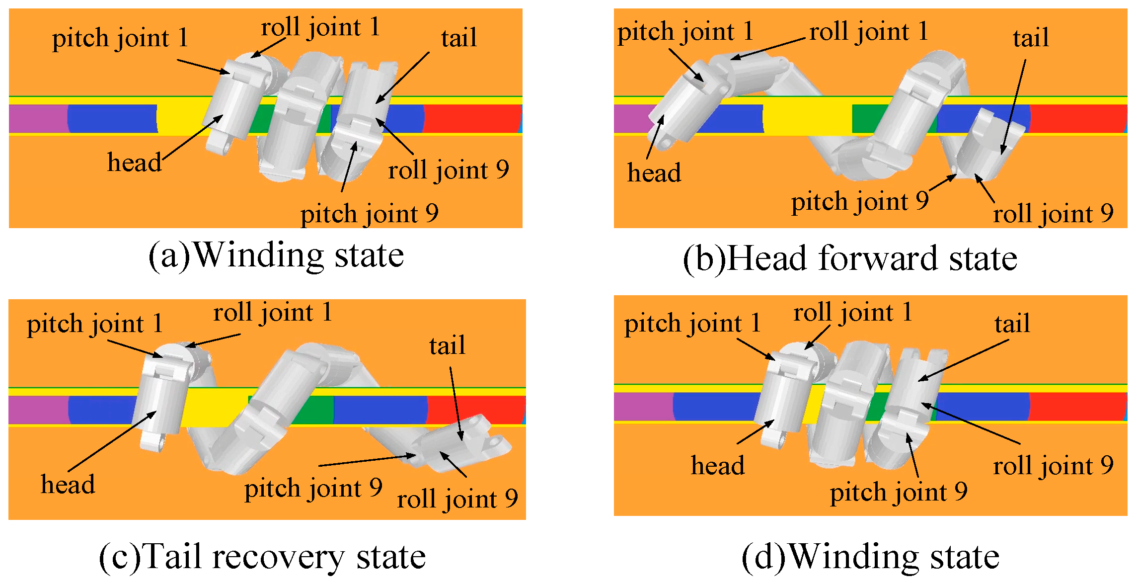
2.1. Conformation and Gait Analysis of the Snake Robot

Figure 1 presents a snake robot model comprising 10 units in series, with each having a pitch joint and a roll joint.

Table 1. Snake robot model parameters.

Parameter	Value
Number of snake robot units $N_s$	10
Length of each unit $l_{link}$	105 mm
Radius of each unit $r_s$	31.5 mm
Pitch joint mass	1 kg
Roll joint mass	0.5 kg

lists the dimensions of the snake robot.

Take the pitch joint as an example to analyze, and the same for the roll joint. From Figure 2 and Figure 3, it can be concluded that at the $t_0$ moment, all pitch joint angles are ${init}_{\mathrm{P}}$ (the initial value of the pitch joint angle) and the snake robot is wrapped around the cable in a winding state (Figure 3a); at the $t_1$ moment, the angle of pitch joint 1 turns to ${min}_{\mathrm{P}}$ (minimum value of the pitch joint angle), the pitch joint 9 angle is still ${init}_{\mathrm{P}}$, and the snake robot’s body reaches as far as it can (Figure 3b); at the $t_2$ moment, the pitch joint 1 angle returns to ${init}_{\mathrm{P}}$, the pitch joint 9 angle turns to ${min}_{\mathrm{P}}$, and the snake robot is in the tail recovery state (Figure 3c); at the $t_3$ moment, all pitch joint angles are ${init}_{\mathrm{P}}$ and the snake robot returns to the winding state (Figure 3d).

2.2. Confirmation of the Joint Angle of the Snake Robot

Establish the coordinate system according to the configuration of the snake robot, as shown in Figure 4. To ease processing the calculation results, a unit is added to the head of the snake robot as a base.

The node is at the connection of two unit sections. Considering the base of the snake robot as the reference, the position of node $w$ is $L_w$:

$$L_w=\frac{w{L}_s}{N_s}$$

(1)

where $N_s$ is the number of body units of the snake robot and $L_s$ is the total length of the snake robot.

The steps to calculate the angle of each joint during the crawling of the snake robot along the cable are as follows:

Step 1: Model the kinematics of the snake robot. According to the coordinate system in Figure 4, the rotation transformation matrix is:

$$\left\{\begin{array}{c}{}_1{}^{h}R=\left[\begin{array}{ccc}cos{\alpha }_i& -sin{\alpha }_i& 0\\ sin{\alpha }_i& cos{\alpha }_i& 0\\ 0& 0& 1\end{array}\right]\\ {}_{j+1}{}^{j}R=\left[\begin{array}{ccc}cos{\alpha }_i& -sin{\alpha }_i& 0\\ 0& 0& -1\\ sin{\alpha }_i& cos{\alpha }_i& 0\end{array}\right]\\ {}_{j+2}{}^{j+1}R=\left[\begin{array}{ccc}cos{\alpha }_i& -sin{\alpha }_i& 0\\ 0& 0& 1\\ -sin{\alpha }_i& -cos{\alpha }_i& 0\end{array}\right]\end{array}\right.$$

(2)

where $j=1, 3, 5, 7\dots \dots {,\alpha }_i$ is the angle of joint $i$. The equation for converting the coordinates of a point $p$ on the snake robot between the joint coordinate system i and the reference coordinate system (coordinate system h) is:

$$p^h={}_i{}^{h}R\times p^i$$

(3)

When $p^i={\left(\begin{array}{ccc}0& 1& 0\end{array}\right)}^T$ ($i$ is an even number), $p^h$ can be considered as the pose of the snake robot unit with respect to the reference coordinate system.

Step 2: Analyze the equation of a cylindrical helix, given by:

$$\left\{\begin{array}{c}x=rcoq\\ y=rsinq\\ z=\frac{h}{2\pi }q\\ h=\frac{\sqrt{{L_s}^2-{\left(r{\theta }_c\right)}^2}}{T_s}\\ {\theta }_c=2\pi T_s \\ r=\frac{r_t+r_s}{cos(\frac{{\theta }_c}{2N_s})}\end{array}\right.$$

(4)

where $r$ is the radius of the helix;$r_t$ is the cable radius; $r_s$ is the unit radius of the snake robot; $h$ is the lead of the helix; $q$ is the radian of point Q on the helix;$L_s$ is the length of the helix and also the full length of the snake robot;${\theta }_c$ is the spiral radian of the helix and also the winding radian of the snake robot; and ${ T}_s$ is the number of winding turns. The helix is illustrated in Figure 5.

Taking the derivative of equations x, y, and z in Equation (4) concerning q, we obtain:

$$\left\{\begin{array}{c}{x}^{\prime }=-rsinq\\ y^{\prime }=rcosq \\ z^{\prime }=\frac{h}{2\pi } \end{array}\right.$$

(5)

A vector can be obtained from Equation (5). This vector is the body pose of the snake robot at the point Q with respect to the reference coordinate system.

Step 3: Find the pose of each unit of the snake robot. The radian $q_w$ corresponding to node $w$ is:

$$q_w=L_w{\theta }_c/L_{s}v$$

(6)

Then, by placing $q_w$, $r_t$, $r_s$, $L_s$, and the winding radian of the snake robot ${\theta }_{init}$ into Equation (5), the corresponding pose of the unit at this node can be obtained as:

$$G_w=\left[\begin{array}{c}{x}^{\prime }\\ y^{\prime }\\ z^{\prime }\end{array}\right]=\left[\begin{array}{c}-rsin{q}_w\\ rcos{q}_w\\ \frac{h}{2\pi }\end{array}\right]$$

(7)

Step 4: Find the initial value of the pitch joint angle ${init}_{\mathrm{P}}$ and the initial value of the roll joint angle ${init}_{\mathrm{R}}$. From Equations (3) and (7), the system of equations is as follows, with $f$ being a scale factor.

$$\left\{\begin{array}{c}{G}_w=f{}_i{}^{h}R\times p^i \\ f>0 \\ i=2w+2\\ p^i={\left(\begin{array}{ccc}0& 1& 0\end{array} \right)}^T\end{array}\right.$$

(8)

According to the limitation of the joint rotation angle, a set of suitable schemes is obtained from Equation (8) as the initial values of pitch joint angle ${init}_{\mathrm{P}}$ and roll joint angle ${init}_{\mathrm{R}}$.

Step 5: Determine the minimum value of the pitch joint angle ${min}_{\mathrm{P}}$ and the maximum value of the roll joint ${max}_{\mathrm{R}}$. Replace ${\theta }_{init}$ with ${\theta }_c;$ repeat steps 3 and 4.

${\theta }_c$ is less than ${\theta }_{init}$, because the length of the helix is equal to the length of the snake robot; when ${\theta }_c$ is smaller than ${\theta }_{init}$, it causes the lead $h$ of the helix to become larger and the helix to elongate. This allows the snake robot to extend its body and crawl along the cable. The larger the difference between ${\theta }_c$ and ${\theta }_{init}$, the longer the step length of the spiral-winding gait of the snake robot.

3. Mathematical Model of Double-Chain Hopf Oscillator

3.1. Mathematical Model of Hopf Oscillator

The Hopf oscillator equation is given by:

$$\left(\begin{array}{c}\dot{u}\\ \dot{v}\end{array}\right)=\left(\begin{array}{c}\mu \left(\rho -r^2\right)u-\omega kv\\ \mu \left(\rho -r^2\right)v+\omega ku\end{array}\right)+\left(\begin{array}{c}{p}_u\\ p_v\end{array}\right)$$

(9)

$$k=\left\{\begin{array}{c}0 \mathrm{Timer} \mathrm{is} \mathrm{working}\\ 1 \mathrm{Timer} \mathrm{is} \mathrm{not} \mathrm{working}\end{array}\right.$$

(10)

Equivalently,

$$\dot{x}=f\left(x;\mu ,\rho ,\omega ,k\right)=\mathrm{F}\left(x\right),x={\left(\begin{array}{cc}u& v\end{array}\right)}^T$$

(11)

where $\sqrt{\rho }$ is the amplitude; $\mu$ is the attraction rate; $\omega$ is the frequency; $u$ and $v$ are the output of the oscillator; $p_u$ and $p_v$ are the coupling terms; and $k$ is the pause enable parameter. This paper uses a timer to change the value of $k$ to make the oscillator pause, with the control logic presented in Figure 6. When the output $v$ of the oscillator equals 1, the timer starts timing, $k$ turns into 0, and the oscillator pauses; when the timer time equals $t_s$ ($t_s$ is the duration of oscillator pause), the timer stops working, the timer is reset, $k$ transforms to 1, and the oscillator continues to move.

The parameters for Equation (9) are set as $\rho$ = 1, $\omega =\pi /4$, and $\mu$ = 100. Additionally, $t_s$ is set as 4 s. During a cycle, the signal value in Figure 7a first decreases, then increases, and finally remains constant; this is the same pattern as the change in pitch joint angle of the snake robot in Figure 2a. Similarly, the pattern of the oscillator output $-v$ change in Figure 7b is the same as the angle change of the roll joint of the snake robot in Figure 2b.

3.2. Structure of the Double-Chain Hopf Controller

The double-chain Hopf oscillator is selected according to the snake robot configuration (Figure 1). The structure of the double-chain Hopf oscillator is depicted in Figure 8.

In the double-chain model, the oscillator of the left chain generates the pitch joint control signal and the oscillator of the right chain generates the roll joint control signal. Bi-directional coupling is used between the oscillators, because when changing the parameters of the oscillator, the bi-directional coupling reaches stability faster than the unidirectional coupling.

The math model of the left chain oscillator is:

$$\left\{\begin{array}{c}{\dot{x}}_{\mathrm{L}i}=\mathrm{F}\left(x_{\mathrm{L}i}\right)-\gamma b_{\mathrm{L}i}\left(x_{\mathrm{L}i}-T_{\mathrm{L}i}^{-1}{x}_{\mathrm{L}i+1}\right)-h\left(x_{\mathrm{R}i}\right), i=1\\ \begin{array}{c}{\dot{x}}_{\mathrm{L}i}=\mathrm{F}\left(x_{\mathrm{L}i}\right)-\gamma a_{\mathrm{L}i-1}\left(x_{\mathrm{L}i}-T_{\mathrm{L}i-1}{x}_{\mathrm{L}i-1}\right)-h\left(x_{\mathrm{R}i}\right),i=n\\ {\dot{x}}_{\mathrm{L}i}=\mathrm{F}\left(x_{\mathrm{L}i}\right)-\gamma \left[b_{\mathrm{L}i}\left(x_{\mathrm{L}i}-T_{\mathrm{L}i}^{-1}{x}_{\mathrm{L}i+1}\right)+a_{\mathrm{L}i-1}\left(x_{\mathrm{L}i}-T_{\mathrm{L}i-1}{x}_{\mathrm{L}i-1}\right)\right]\\ -h\left(x_{\mathrm{R}i}\right),1<i<n\end{array}\end{array}\right.$$

(12)

where $\mathrm{L}i$ is the number of the left side oscillator; $T_{\mathrm{L}i}=\frac{\sqrt{{\rho }_{\mathrm{L}i+1}}}{\sqrt{{\rho }_{\mathrm{L}i}}}\left(\begin{array}{cc}cos{\phi }_{\mathrm{L}}& -sin{\phi }_{\mathrm{L}}\\ sin{\phi }_{\mathrm{L}}& cos{\phi }_{\mathrm{L}}\end{array}\right)$, $\mathrm{w}\mathrm{i}\mathrm{t}\mathrm{h} {\phi }_{\mathrm{L}}$ the phase difference between two adjacent oscillators on the left side; $\mathsf{\gamma }$ is the overall coupling gain; $a_{\mathrm{L}i}$ is the left side oscillator’s coupling strength in the rostral direction, $\mathrm{w}\mathrm{i}\mathrm{t}\mathrm{h} a_{\mathrm{L}i}=\left\{\begin{array}{c}1 k_{\mathrm{L}i}+k_{\mathrm{L}i-1}=2\\ 0 k_{\mathrm{L}i}+k_{\mathrm{L}i-1}<2\end{array}\right.$; $b_{\mathrm{L}i}$ is the left side oscillator’s coupling strength in the caudal direction,${\mathrm{w}\mathrm{i}\mathrm{t}\mathrm{h} b}_{\mathrm{L}i}=\left\{\begin{array}{c}1 k_{\mathrm{L}i}+k_{\mathrm{L}i+1}=2\\ 0 k_{\mathrm{L}i}+k_{\mathrm{L}i+1}<2\end{array}\right.$; $h\left(x_{\mathrm{R}i}\right)$ is the right-hand side coupling term, $\mathrm{w}\mathrm{i}\mathrm{t}\mathrm{h} h\left(x_{\mathrm{R}i}\right)=e_i\left(x_{\mathrm{L}i}-T_{\mathrm{m}i}^{-1}{x}_{\mathrm{R}i}\right)$,$T_{\mathrm{m}i}=\frac{\sqrt{{\rho }_{\mathrm{R}i}}}{\sqrt{{\rho }_{\mathrm{L}i}}}\left(\begin{array}{cc}cos{\phi }_{\mathrm{m}}& -sin{\phi }_{\mathrm{m}}\\ sin{\phi }_{\mathrm{m}}& cos{\phi }_{\mathrm{m}}\end{array}\right)$, ${\mathrm{a}\mathrm{n}\mathrm{d} \phi }_{\mathrm{m}}$ is the phase difference between oscillator $\mathrm{L}i$ and $\mathrm{R}i$; $e_i$ is the coupling strength in the right direction, with $e_i=\left\{\begin{array}{c}1 k_{\mathrm{L}i}+k_{\mathrm{R}i}=2\\ 0 k_{\mathrm{L}i}+k_{\mathrm{R}i}<2\end{array}\right.$; ${\mathrm{a}\mathrm{n}\mathrm{d} k}_{\mathrm{L}i}$ and $k_{\mathrm{R}i}$ are the pause enable parameters of oscillator $\mathrm{L}i$ and oscillator $\mathrm{R}i$.

The right side equations are omitted since they are obvious due to the (L R) symmetry. The structure diagram of the double-chain model is shown in Figure 9.

Combining the joint angles of the snake robot obtained from the Equation (8) calculation, the output of the double-chain Hopf oscillator is:

$$\left\{\begin{array}{c}{y}_{\mathrm{L}i}=\frac{v_{\mathrm{L}i}\left({init}_P-{min}_P\right)}{2}+\frac{\left({init}_P+{min}_P\right)}{2}\\ y_{\mathrm{R}i}=\frac{v_{\mathrm{R}i}\left({max}_R-{init}_R\right)}{-2}+\frac{\left({init}_R+{max}_R\right)}{2}\end{array}\right.$$

(13)

where $v_{\mathrm{L}i}$ is the output of the left side in the double-chain Hopf oscillator and $v_{\mathrm{R}i}$ is the output of the right side in the double-chain Hopf oscillator.

Setting the parameters of the double-chain Hopf oscillator ${init}_P=90°$, ${init}_R=45°$, ${min}_P=45°$, ${max}_R=90°$; the phase difference between adjacent oscillators is ${\phi }_{\mathrm{L}}{=\phi }_{\mathrm{R}}=\pi /4$; the oscillator frequency is $\omega =\pi /2$; the trigger condition for the timer in all Hopf oscillators is that the oscillator output $v_{Li}=v_{Ri}=1$; and oscillator pause oscillation time $t_s=2\hspace{0.17em}\mathrm{s}$. The output signal is shown in Figure 10. The output signal of the oscillator right chain is consistent with the variation law of the roll joint angle of the snake robot, as shown in Figure 10a; the output signal of the oscillator left chain is consistent with the variation law of the pitch joint angle of the snake robot, as shown in Figure 10b. The phase difference between the same numbered oscillators in the left chain and the right chain is 0; for example, the phase difference between oscillator R₁ and oscillator L₁ is 0; this also satisfies the characteristic that the time difference between the pitch joint and the roll joint motion of the same snake robot unit is 0.

4. Simulation

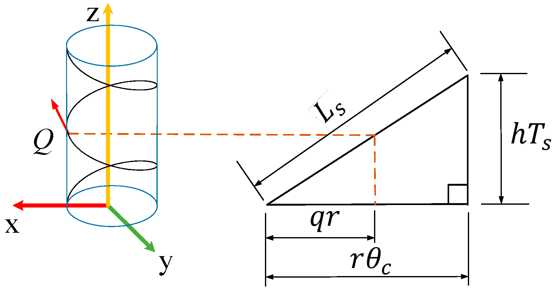
4.1. Spiral-Winding Gait

From the snake robot gait analysis in Figure 2, the phase difference between the head joint and the tail joint of the snake robot is $\pi ;$ therefore, the phase difference between adjacent oscillators on the same side is $\pi /(N_s-2)$, the phase difference between the left and right oscillators is 0, and the oscillator pause time $t_s=\pi /\omega$ seconds. The trigger condition for the timer in all Hopf oscillators is that the oscillator unit output $v_{Li}=v_{Ri}=1$. The detailed parameters of the dual-chain Hopf oscillator are shown in

Table 2. Oscillator parameters.

Parameter	Value
Opposite-side phase difference ${\phi }_{\mathrm{m}}$	0
Same-side phase difference ${\phi }_{\mathrm{L}}$ and ${\phi }_R$	$\pi /8$
Overall coupling gain $\gamma$	1
Amplitude $\sqrt{\rho }$	1
Attraction rate $\mu$	100
Frequency of the oscillator $\omega$	$\pi /4$
Duration of oscillator pause $t_s$	4 s

.

The controller can change the step length of the snake robot by changing the crawling angle of its joint. The cable radius $r_t=25.5\mathrm{mm}$ and the dimensions of the snake robot are shown in Table 1. Bring the winding radius ${\theta }_{init}=14.8 \mathrm{r}\mathrm{a}\mathrm{d}$ into Equation (8), then ${init}_R$(initial angle of roll joint) is 18.21° and ${init}_P$(initial angle of pitch joint) is 83.02°. During the first gait cycle, bring the winding radius ${\theta }_{c1}=13.2 \mathrm{r}\mathrm{a}\mathrm{d}$ into Equation (8), ${\mathrm{t}\mathrm{h}\mathrm{e}\mathrm{n} max}_R$(maximum value of roll joint) is 40.49° and ${min}_P$(minimum value of pitch joint) is 65.25°. During the second gait cycle, bring the winding radius ${\theta }_{c2}=12.6 \mathrm{r}\mathrm{a}\mathrm{d}$ into Equation (8), ${\mathrm{t}\mathrm{h}\mathrm{e}\mathrm{n} max}_R$ is 43.3° and ${min}_P$ is 59.02°. Figure 11 shows the motion process of the snake robot with variable step lengths. Figure 12 shows the angular variation of the snake robot joints.

In Figure 12, some of the joint angles appear to be fluctuating. The reason is that this paper makes an approximation of the calculation of the motion angle of the snake robot joints, causing the spiral winding radius of the snake robot to be slightly larger than the cable radius. During the motion process, there is an angle between the axis of spiral winding of the snake robot and the cable axis, which leads to a deviation of the winding attitude of the snake robot and makes some of the joints’ motion restricted, together with the influence of the front joint movement, causing some of the joint angles to appear to be fluctuating.

As shown in Figure 12, the winding radian ${\theta }_{init}$ of the snake robot is used to find the ${init}_R$ (initial angle of roll joint) and the ${init}_P$ (initial angle of pitch joint). The winding arc ${\theta }_c$ is used to find the ${max}_R$ (maximum value of roll joint) and the ${min}_P$ (minimum value of pitch joint) of the snake robot. ${\theta }_c$ is smaller than ${\theta }_{init};$ the larger the difference between ${\theta }_{init}$ and ${\theta }_c$, the longer the step length of the spiral-winding gait of the snake robot, and the faster the crawling speed of the snake robot along the cable.

In this paper, the crawling speed of the snake robot along the cable with different friction coefficients will be measured by varying the value of ${\theta }_c$. Setting ${\theta }_{init}=14.8 \mathrm{r}\mathrm{a}\mathrm{d}$, and taking ${\theta }_c$ as $12.2 \mathrm{r}\mathrm{a}\mathrm{d}$, $12.4 \mathrm{r}\mathrm{a}\mathrm{d},12.6 \mathrm{r}\mathrm{a}\mathrm{d},12.8 \mathrm{r}\mathrm{a}\mathrm{d},13 \mathrm{r}\mathrm{a}\mathrm{d}$, $\mathrm{a}\mathrm{n}\mathrm{d} 13.2 \mathrm{r}\mathrm{a}\mathrm{d}$, the parameters of the double-chain Hopf oscillator are listed in Table 2, but the frequency $\omega$ is changed to $\pi /2$ and the oscillator pause duration $t_s$ is changed to 2 s. The speed of the snake robot crawling along the cable is measured at friction coefficients of 0.3, 0.4, 0.5, and 0.6, respectively. The relationship between the winding arc ${\theta }_c$ of the snake robot and the crawling speed is obtained by polynomial fitting, as shown in Figure 13.

In Figure 13, the maximum speeds of the snake robot crawling along the cable at the cable friction coefficients of 0.3, 0.4, 0.5, and 0.6 are 1.0465 cm/s; 0.9565 cm/s, 0.9534 cm/s, and 0.894 cm/s, respectively. It can also be observed from Figure 13 that the larger the cable friction coefficient, the smaller the crawling speed of the snake robot along the cable; this is because the higher the coefficient friction of the cable, the larger the resistance to the movement of the snake robot unit, and the slower the robot crawls.

Furthermore, the larger the value of ${\theta }_{init}-{\theta }_c$, the longer the motion step length and the faster the crawling speed of the snake robot. But when the value of ${\theta }_{init}-{\theta }_c$ is large to a certain extent, and if continuing to reduce the value of ${\theta }_c$, the increase in the crawling speed of the snake robot is smaller and the larger ${\theta }_{init}-{\theta }_c$ is, the longer the snake robot motion step is and the easier it is for the robot to slip off the cable.

Therefore, in this paper, the SAA (Simulated Annealing Algorithm) is used to find the optimal step length of the spiral-winding gait of the snake robot by adjusting the winding arc ${\theta }_c$ to improve the crawling speed of the snake robot along the cable.

4.2. Optimization of the Crawling Speed of the Snake Robot

With ${\theta }_{init}$ held constant, the SAA (Simulated Annealing Algorithm) is used to find the appropriate ${\theta }_c$ by comparing the increase of the robot’s crawling speed. Therefore, in this paper, the judgment condition of the SAA is set according to the increment of crawling speed, and the purpose is to make the optimized snake robot crawling speed close to the maximum speed in Figure 13, and not make the step length too long. The flowchart of the SAA is illustrated in Figure 14 and involves the following process:

Step 1: Given the winding arc ${\theta }_{init}$ and ${\theta }_{c1}$, the crawling distance $Y_0$ is obtained after the snake robot runs for three gait cycles based on position information.

Step 2: The winding radian ${\theta }_{c2}$ is obtained by ${\theta }_{c2}=z{\theta }_{c1}$, where $z$ is the decay parameter. After the snake robot runs for three gait cycles of time, the distance $Y_1$ of crawling is obtained based on the position information.

Step 3. Determine whether to accept the winding radian ${\theta }_{c2}$. Since the gait period is constant, the distance of crawling can also reflect the speed of crawling. The judgment condition is $Y_1-Y_0=0.225Y_0$. If this condition is satisfied, the winding radian ${\theta }_{c2}$ is accepted, the number of iterations $I$ is cleared to zero, and step 5 is executed. If the condition is not satisfied, step 4 is executed.

Step 4: Follow the Metropolis criterion to decide whether to accept the winding radian ${\theta }_{c2}$. If the criterion is satisfied, the winding radian ${\theta }_{c2}$ is accepted, the iterations $I$ is cleared, and step 5 is executed. If not, add one to the original number of iterations $I$ and execute step 5.

Step 5. Determine whether the number of iterations $I$ is higher than 4. If $I$ is higher than 4, end the annealing process and output the final crawling speed. Otherwise, execute step 2.

The parameters of the double-chain Hopf oscillator are listed in Table 2, but the frequency $\omega$ is changed to $\pi /2$ and the oscillator pause duration $t_s$ is changed to 2 s. The parameters of the SAA are shown in

Table 3. SAA parameters.

Parameter	Value
Winding arc ${\theta }_{init}$	$14.8 \mathrm{r}\mathrm{a}\mathrm{d}$
Winding arc ${\theta }_c$	$13.2 \mathrm{r}\mathrm{a}\mathrm{d}$
Decay parameter $z$	0.99

. The optimization effect of the snake robot’s crawling speed is depicted in Figure 15.

The maximum crawling speeds obtained using the SAA at cable friction coefficients of 0.3, 0.4, 0.5, and 0.6 are 0.8868 cm/s, 0.8843 cm/s, 0.8598 cm/s, and 0.7971 cm/s, respectively. The differences from the maximum velocity in Figure 13 are 18.01%, 8.16%, 11.01%, and 12.16%, respectively. The deviations produced are small and close to the maximum velocity in Figure 13.

In Figure 15, with cable friction coefficients of 0.3, 0.4, 0.5, and 0.6, the ${\theta }_c$ for the snake robot to reach the maximum crawling speed are 12.303 rad, 12.680 rad, 12.428 rad, and 12.533 rad, respectively. These ${\theta }_c$ values are all larger than 12.2 rad, which is the value of ${\theta }_c$ corresponding to the maximum velocity in Figure 13. This means that the snake robot has a smaller step length.

This paper tests the effectiveness of optimizing the snake robot crawling speed with the SAA when the cable tilt angle is 5° or −5°. The friction coefficient of the cable is 0.5.

Setting ${\theta }_{init}=14.8 \mathrm{r}\mathrm{a}\mathrm{d}$ and taking ${\theta }_c$ as $12.2 \mathrm{r}\mathrm{a}\mathrm{d}$, $12.4 \mathrm{r}\mathrm{a}\mathrm{d}$, $12.6 \mathrm{r}\mathrm{a}\mathrm{d}$, $12.8 \mathrm{r}\mathrm{a}\mathrm{d}$, $13 \mathrm{r}\mathrm{a}\mathrm{d}$, $\mathrm{a}\mathrm{n}\mathrm{d} 13.2 \mathrm{r}\mathrm{a}\mathrm{d}$, the parameters of the double-chain Hopf oscillator are listed in Table 2, but the frequency $\omega$ is changed to $\pi /2$ and the oscillator pause duration $t_s$ is changed to 2 s. The speed of a snake robot crawling along a cable with an inclination of 5° or −5° is shown in Figure 16.

The maximum crawling speed of the snake robot is 0.453 cm/s and 1.241 cm/s when the cable inclination angle is 5° and −5°, respectively. The smaller the inclination of the cable, the faster the snake robot crawls.

The parameters of the SAA are shown in Table 3. The optimization effect of the snake robot’s crawling speed is depicted in Figure 17.

When the inclination angle of the cable is 5° and −5°, the speed of the snake robot crawling along the cable after optimization with the SAA is 0.421 cm/s and 1.124 cm/s, respectively, and the winding arcs are $12.81 \mathrm{r}\mathrm{a}\mathrm{d}$ and $12.55 \mathrm{r}\mathrm{a}\mathrm{d},$ respectively. The differences from the maximum velocity in Figure 16 are 7.6% and 10.4%, respectively, and the snake robot has a smaller step length.

This paper also conducts simulation experiments for another size of cable to verify the effectiveness of the method proposed in this paper, where the radius of the cable is 20.5 cm.

As the radius of the cable changes, the winding arc of the snake robot also changes. Setting ${\theta }_{init}=15.7 \mathrm{r}\mathrm{a}\mathrm{d}$ and taking ${\theta }_c$ as $15 \mathrm{r}\mathrm{a}\mathrm{d}$, $14.5 \mathrm{r}\mathrm{a}\mathrm{d}$, $14 \mathrm{r}\mathrm{a}\mathrm{d}$, $13.5 \mathrm{r}\mathrm{a}\mathrm{d}$, $13 \mathrm{r}\mathrm{a}\mathrm{d}$, $12.5 \mathrm{r}\mathrm{a}\mathrm{d}$, $\mathrm{a}\mathrm{n}\mathrm{d} 12 \mathrm{r}\mathrm{a}\mathrm{d}$, the parameters of the double-chain Hopf oscillator are listed in Table 2, but the frequency $\omega$ is changed to $\pi /2$ and the oscillator pause duration $t_s$ is changed to 2 s. The crawling speed of the snake robot along the cable is shown in Figure 18.

In Figure 18, the maximum speeds of the snake robot crawling along the cable at the cable friction coefficients of 0.3, 0.4, 0.5, and 0.6 are 0.8946 cm/s, 0.8269 cm/s, 0.7956 cm/s, and 0.7336 cm/s, respectively.

The parameters of the SAA are shown in Table 3. The optimization effect of the snake robot’s crawling speed is depicted in Figure 19.

The maximum crawling speeds obtained using the SAA at cable friction coefficients of 0.3, 0.4, 0.5, and 0.6 are 0.8046 cm/s, 0.7592 cm/s, 0.7004 cm/s, and 0.6891 cm/s, respectively. The differences from the maximum velocity in Figure 18 are 11.18%, 8.9%, 13.59%, and 6.45%, respectively. The deviations produced are small and close to the maximum velocity in Figure 18.

In Figure 18, with cable friction coefficients of 0.3, 0.4, 0.5, and 0.6, the ${\theta }_c$ for the snake robot to reach the maximum crawling speed are 13.43 rad, 13.56 rad, 13.70 rad, and 13.16 rad, respectively. These ${\theta }_c$ values are all larger than 12 rad, which is the value of ${\theta }_c$ corresponding to the maximum velocity in Figure 18.

All of the above experiments demonstrate that using the SAA (Simulated Annealing Algorithm) can help find an optimal step length that allows the snake robot to have a high crawling speed and not slip easily from the cable.

5. Discussion

In this paper, a spiral-winding gait is designed for the cable inspection task of the snake robot which is composed of P-R units, and according to the motion characteristics of this gait, a double-chain Hopf oscillator is proposed as a gait controller for the robot. By adjusting the parameters of the dual-chain Hopf oscillator, a “ change–maintain–change …… “ periodic signal can be output to control the snake robot to crawl along the cable. This paper investigates the effects of the cable friction coefficient and cable tilt angle on the crawling speed of the snake robot, with the simulation results showing that when the motion step length of the snake robot is fixed, the larger the cable friction coefficient and cable tilt angle, the slower the crawling speed of the snake robot. The simulation results also show that when the cable friction coefficient, cable tilt angle, and cable diameter are fixed, the longer the step length of the spiral-winding gait of the snake robot, the faster the robot crawls;, in addition, the smaller the increase in robot crawling speed, also the longer the motion step of the snake robot, the easier it is for the snake robot to slip off the cable. Therefore, in order to make the snake robot have both high crawling speed and for it to be difficult to slip off the cable, this paper takes the speed increase as the determination basis and uses the SAA to search for the optimal step length of the spiral-winding gait of the snake robot, with the simulation result showing that using the SAA to search for the optimal step length of the spiral-winding gait of the snake robot is effective.

But these jobs do not yet allow the snake robot to patrol along the cable. There are also many obstacles on the cable, and the current gait controller is not accurate enough to control the crawling speed of the snake robot. Therefore, the next research task is to design crossing gaits for various obstacles on the cable and to design a set of feedback control networks for the dual-chain Hopf oscillator to improve the accuracy of crawling speed control for the snake robot.

References

1. Liljebäck, P.; Pettersen, K.Y.; Stavdahl, Ø.; Gravdahl, J.T. A review on modelling, implementation, and control of snake robots. Robot. Auton. Syst. 2012, 60, 29–40. [Google Scholar] [CrossRef] [Green Version]
2. Stamper, S.A.; Sefati, S.; Cowan, N.J. Snake robot uncovers secrets to sidewinders’ maneuverability. Proc. Natl. Acad. Sci. USA 2015, 112, 5870–5871. [Google Scholar] [CrossRef] [PubMed]
3. Girma, A.; Bahadori, N.; Sarkar, M.; Tadewos, T.G.; Behnia, M.R.; Mahmoud, M.N.; Karimoddini, A.; Homaifar, A. IoT-Enabled Autonomous System Collaboration for Disaster-Area Management. IEEE/CAA J. Autom. Sin. 2020, 7, 1249–1262. [Google Scholar] [CrossRef]
4. Yang, L.; Li, B.; Li, W.; Brand, H.; Jiang, B.; Xiao, J. Concrete defects inspection and 3D mapping using CityFlyer quadrotor robot. IEEE/CAA J. Autom. Sin. 2020, 7, 991–1002. [Google Scholar] [CrossRef]
5. Cao, Z.; Zhang, D.; Zhou, M. Direction Control and Adaptive Path Following of 3-D Snake-Like Robot Motion. IEEE Trans. Cybern. 2021, 52, 10980–10987. [Google Scholar] [CrossRef] [PubMed]
6. Ariizumi, R.; Matsuno, F. Dynamic Analysis of Three Snake Robot Gaits. IEEE Trans. Robot. 2017, 33, 1075–1087. [Google Scholar] [CrossRef]
7. Grillner, S. Biological Pattern Generation: The Cellular and Computational Logic of Networks in Motion. Neuron 2006, 52, 751–766. [Google Scholar] [CrossRef] [PubMed] [Green Version]
8. Yu, J.; Tan, M.; Chen, J.; Zhang, J. A Survey on CPG-Inspired Control Models and System Implementation. IEEE Trans. Neural Netw. Learn. Syst. 2014, 25, 441–456. [Google Scholar] [CrossRef] [PubMed]
9. Nor, N.M.; Ma, S. Smooth transition for CPG-based body shape control of a snake-like robot. Bioinspir. Biomim. 2014, 9, 016003. [Google Scholar] [CrossRef] [PubMed]
10. Wang, Z.; Gao, Q.; Zhao, H. CPG-Inspired Locomotion Control for a Snake Robot Basing on Nonlinear Oscillators. J. Intell. Robot. Syst. 2017, 85, 209–227. [Google Scholar] [CrossRef]
11. Fujiki, S.; Aoi, S.; Yamashita, T.; Funato, T.; Tomita, N.; Senda, K.; Tsuchiya, K. Adaptive splitbelt treadmill walking of a biped robot using nonlinear oscillators with phase resetting. Auton. Robots 2013, 35, 15–26. [Google Scholar] [CrossRef] [Green Version]
12. Kimura, H.; Fukuoka, Y.; Cohen, A.H. Adaptive Dynamic Walking of a Quadruped Robot on Natural Ground Based on Biological Concepts. Int. J. Robot. Res. 2007, 26, 475–490. [Google Scholar] [CrossRef]
13. Ijspeert, A.J.; Crespi, A.; Ryczko, D.; Cabelguen, J.M. From Swimming to Walking with a Salamander Robot Driven by a Spinal Cord Model. Science 2007, 315, 1416–1420. [Google Scholar] [CrossRef] [PubMed] [Green Version]
14. Wu, X.; Ma, S. Adaptive creeping locomotion of a CPG-controlled snake-like robot to&nbsp;environment change. Auton. Robot. 2010, 28, 283–294. [Google Scholar]
15. Cao, Z.; Zhang, D.; Hu, B.; Liu, J. Adaptive Path Following and Locomotion Optimization of Snake-Like Robot Controlled by the Central Pattern Generator. Complexity 2019, 2019, 8030374. [Google Scholar] [CrossRef] [Green Version]
16. Manzoor, S.; Choi, Y. A unified neural oscillator model for various rhythmic locomotions of snake-like robot. Neurocomputing 2016, 173, 1112–1123. [Google Scholar] [CrossRef]
17. Miao, H.; Tian, Y.C. Dynamic robot path planning using an enhanced simulated annealing approach. Appl. Math. Comput. 2013, 222, 420–437. [Google Scholar] [CrossRef] [Green Version]
18. Kwok, D.P.; Sheng, F. Genetic algorithm and simulated annealing for optimal robot arm PID control. In Proceedings of the First IEEE Conference on Evolutionary Computation. IEEE World Congress on Computational Intelligence, Orlando, FL, USA, 27–29 June 1994; pp. 707–713. [Google Scholar]
Figure 1. Snake robot model.
Electronics 12 03094 g001
Figure 2. (a,b) Gait timing diagram of the snake robot.
Electronics 12 03094 g002
Figure 3. (ad) Attitude change of the snake robot in one cycle.
Electronics 12 03094 g003
Figure 4. Snake robot coordinate system.
Electronics 12 03094 g004
Figure 5. Cylindrical helix.
Electronics 12 03094 g005
Figure 6. Timer control flowchart.
Electronics 12 03094 g006
Figure 7. Hopf oscillator output versus time: (a) is oscillator output v versus time curve, (b) is oscillator output −v versus time curve.
Electronics 12 03094 g007
Figure 8. Structure of the double-chain CPG controller: (a) is bi-directional connection, (b) is unidirectional connection.
Electronics 12 03094 g008
Figure 9. Double-chain model structure diagram.
Electronics 12 03094 g009
Figure 10. Output of double-chain Hopf oscillator: (a) is Oscillator right chain output, (b) is Oscillator left chain output.
Electronics 12 03094 g010
Figure 11. Snake robot change step length motion process.
Electronics 12 03094 g011
Figure 12. Variation curve of joint angle of snake robot: (a) is Roll joint angle change curve, (b) is Pitch joint angle change curve.
Electronics 12 03094 g012
Figure 13. The relationship between the crawling speed and winding arc of the snake robot under different friction environments.
Electronics 12 03094 g013
Figure 14. Flowchart of SAA.
Electronics 12 03094 g014
Figure 15. Variation of crawling speed of the snake robot.
Electronics 12 03094 g015
Figure 16. Crawling speed of the snake robot on cables with different inclination angles.
Electronics 12 03094 g016
Figure 17. The effect of SAA on the optimization of snake robot crawling speed.
Electronics 12 03094 g017
Figure 18. Snake robot crawling speed along the cable.
Electronics 12 03094 g018
Figure 19. Optimization effect of SAA on crawling speed of the snake robot.
Electronics 12 03094 g019