
Bi-Level Optimization Model for DERs Dispatch Based on an Improved Harmony Searching Algorithm in a Smart Grid

Abstract
:1. Introduction
1.1. Literature Review
1.2. Methodology and Organization of the Article
2. Bi-Level Optimization Model
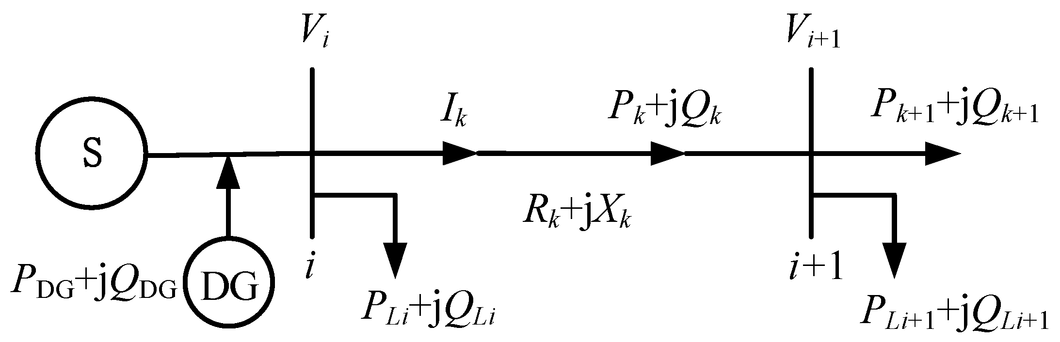
2.1. Upper-Level Aim Function
2.1.1. Determination of DG Position
2.1.2. Determination of DG Capacity
2.2. Lower-Level Aim Function
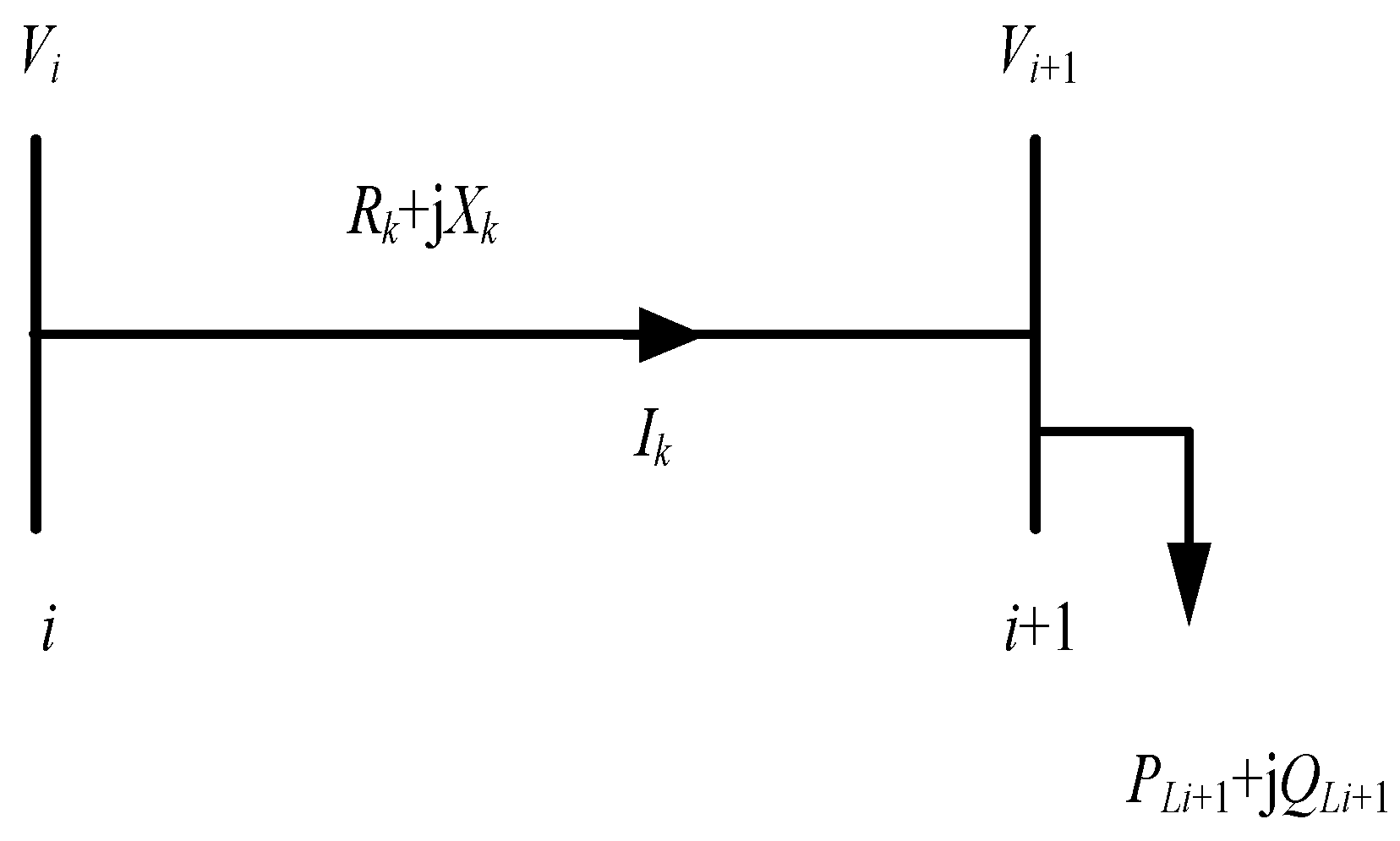
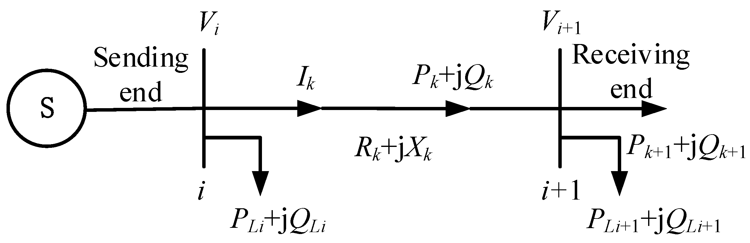
2.2.1. Power Flow Constraint
2.2.2. Node Voltage Constraint
2.2.3. Branch Current Constrain
2.2.4. Network Topology Constraint
3. Coding Principle of Reconfiguration Ring
3.1. Basic Ring Matrix
3.2. Topology Simplification of Distribution Network
- The branches directly connected to the power source node cannot be coded;
- For an independent branch that does not form a loop, if the switch related to it is disconnected, an isolated island will be formed, and so it cannot be coded;
- Based on the knowledge related to node degree, close all the switches in the network. Merge the branches between nodes where the sum of their indegrees and outdegrees is less than or equal to 2 into one branch, which is denoted as a branch group.
3.3. Modification of Infeasible Solution
- Only one branch can be disconnected for each basic ring, otherwise, an isolated island will be formed;
- If multiple basic rings have included relationships, the basic ring with more section switches will be disconnected first. Then, the rings will be broken up in order of their size, with only one branch being disconnected in the public branch group, at most;
- If there are pairwise intersecting relationships between multiple basic rings, with each ring having at least their basic rings, then there will be at least one closed branch in the public branch group;
- If multiple basic rings simultaneously meet the above two conditions, and there is a public branch disconnected between one basic ring and the remaining N-1 basic rings, without including public branch sets of N basic rings, then it may be acceptable for the disconnected branches to exist in the public branches of N basic rings.
4. Discussion
4.1. Improved Harmony Search Algorithm
- Firstly, the HSA includes five parameters: harmony memory (HM), harmony memory size (HMS), harmony memory considering rate (HMCR), pitch adjusting rate (PAR), and bandwidth (bw);
- To initialize the harmony memory, the matrix from HM can be expressed as shown in (20), wherein represents the randomly generated solution vector;
- Improvise a new harmony: There are three main parameters involved in a new generation of harmony vectors, i.e., HMCR, PAR, and bw. Assuming that the new harmony is , and it is then generated below:
- Firstly, to generate a random number rand1 in the range of 0 to 1 following uniformly distributed. If rand1 < HMCR, then the new solution is selected from HM with the rate of HMCR, and denoted by . Otherwise, it is randomly selected from the outside of HM with the rate of (1-HMCR), and denoted by ;
- If the new solution is selected from HM, that is, , then it randomly generates a number rand2 in the range of 0 to 1 following a uniform. If rand , the new solution will be generated according to . Otherwise, it will keep unchanged, that is, .
- Repeat the above steps until a completely new harmony vector is generated;
- Update the harmony memory by comparing the fitness value of the new harmony vector with the worst harmony vector in the HM, and if the fitness value of the new harmony vector is better, it replaces the worst harmony vector; otherwise, the newly generated harmony vector is removed from the HM;
- Check the termination conditions. If the maximum number of iterations has not been reached, repeat steps 3 and 4; otherwise, terminate the process.
- Improvement of parameters: Based on the search mechanism of HSA, during the early stage of optimization, it is recommended to select solution vectors in HM with a larger HMCR and a small PAR, considering the larger search space, whereas in the later period, with the solution vectors updated and the optimized space condensed, the new solution vector in HM need to be selected with smaller HMCR and larger PAR to prevent falling into local optimization. The parameters improvement can be written bywhere is maximum fitness in HM, is minimum fitness in HM, is the average fitness in the whole HM.
- Judgment of local optimization. To enhance the accuracy of the optimization process, more accurate, a local optimal judgment mechanism is added bywhere is the fitness variance of the solution vectors, is the fitness of ith harmony, and is the average of fitness in the whole HM.
4.2. Model Optimization Based on Improving HSA
- Input the original data, preprocess them, and set up the parameters of the improved HAS;
- Determine the installation position and capacity of DGs according to the and in the upper optimization model. These values are used as the solution vector of the upper-level optimization model, save them and the topology of the distribution network in HM;
- Use the solution vector generated in step 2 as the initial value in the lower optimization model. Then, apply the improved HSA to perform the lower-level optimization, which will determine the new distribution network structure. Finally, update the HM with the new information;
- To determine the termination conditions, check if they are satisfied. If the conditions are met, the iteration stops and proceeds to step 5. Otherwise, return to step 2;
- Output the optimized solution vectors.
5. Examples
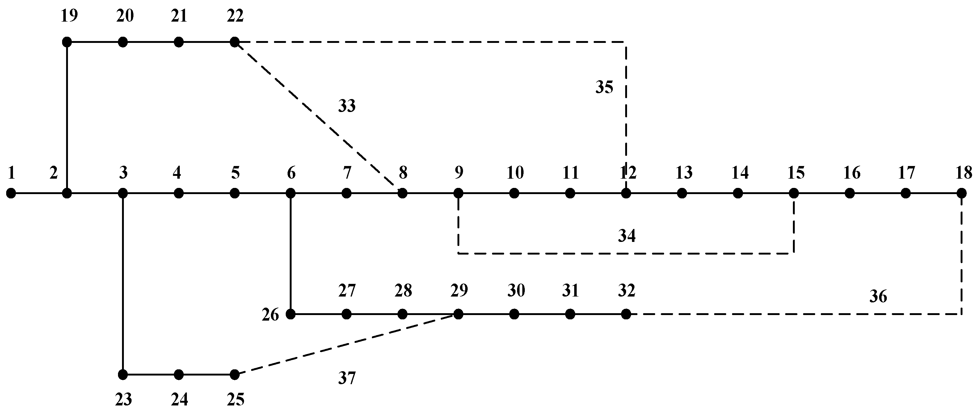
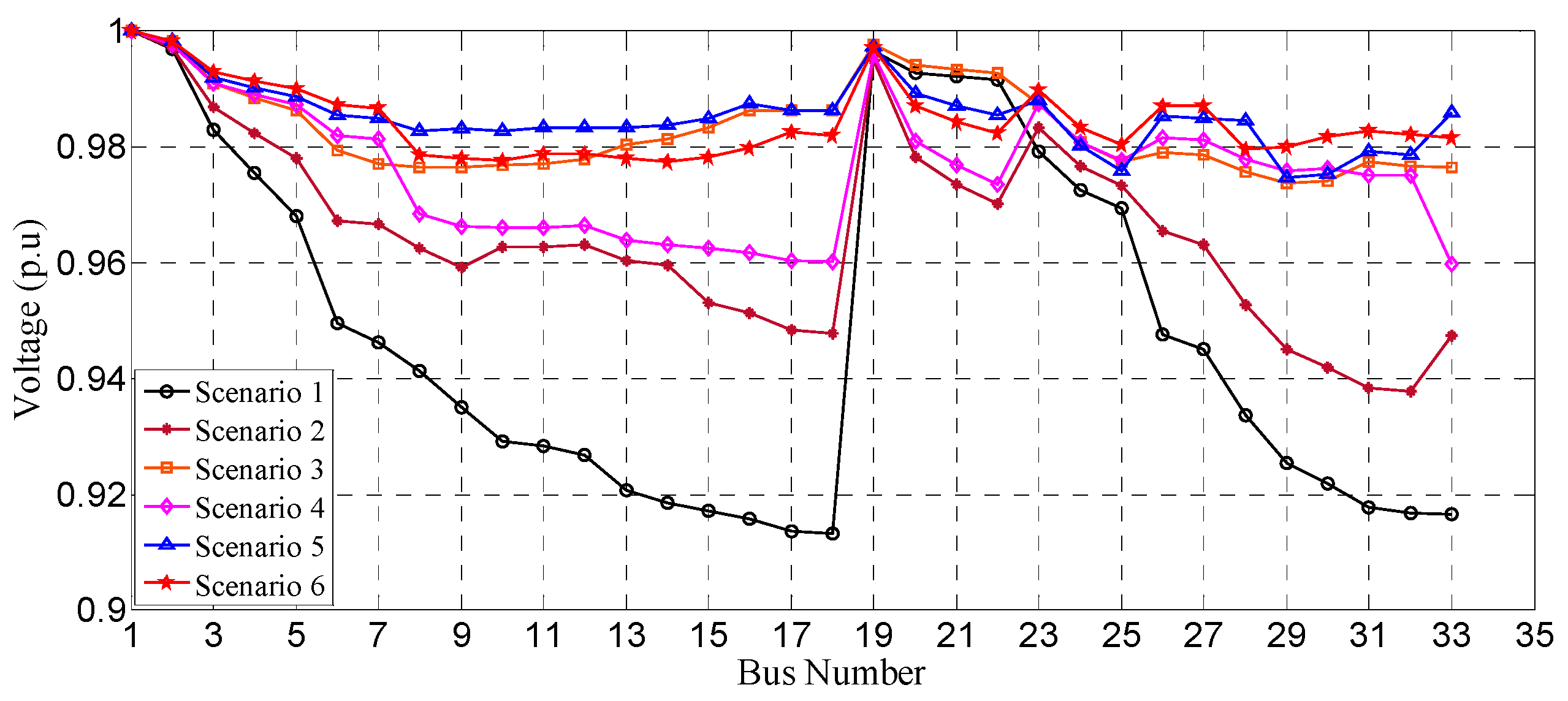
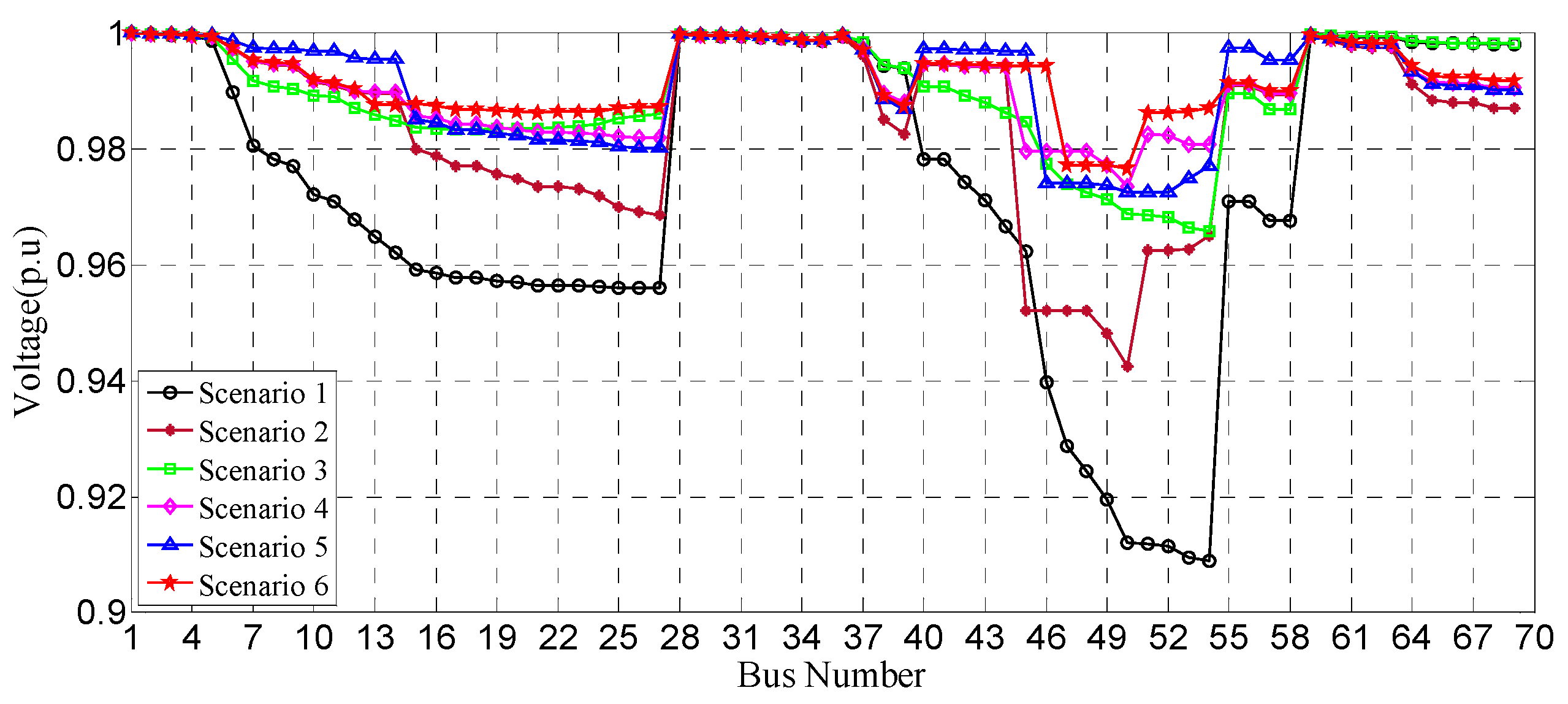
5.1. 33-Bus Test System
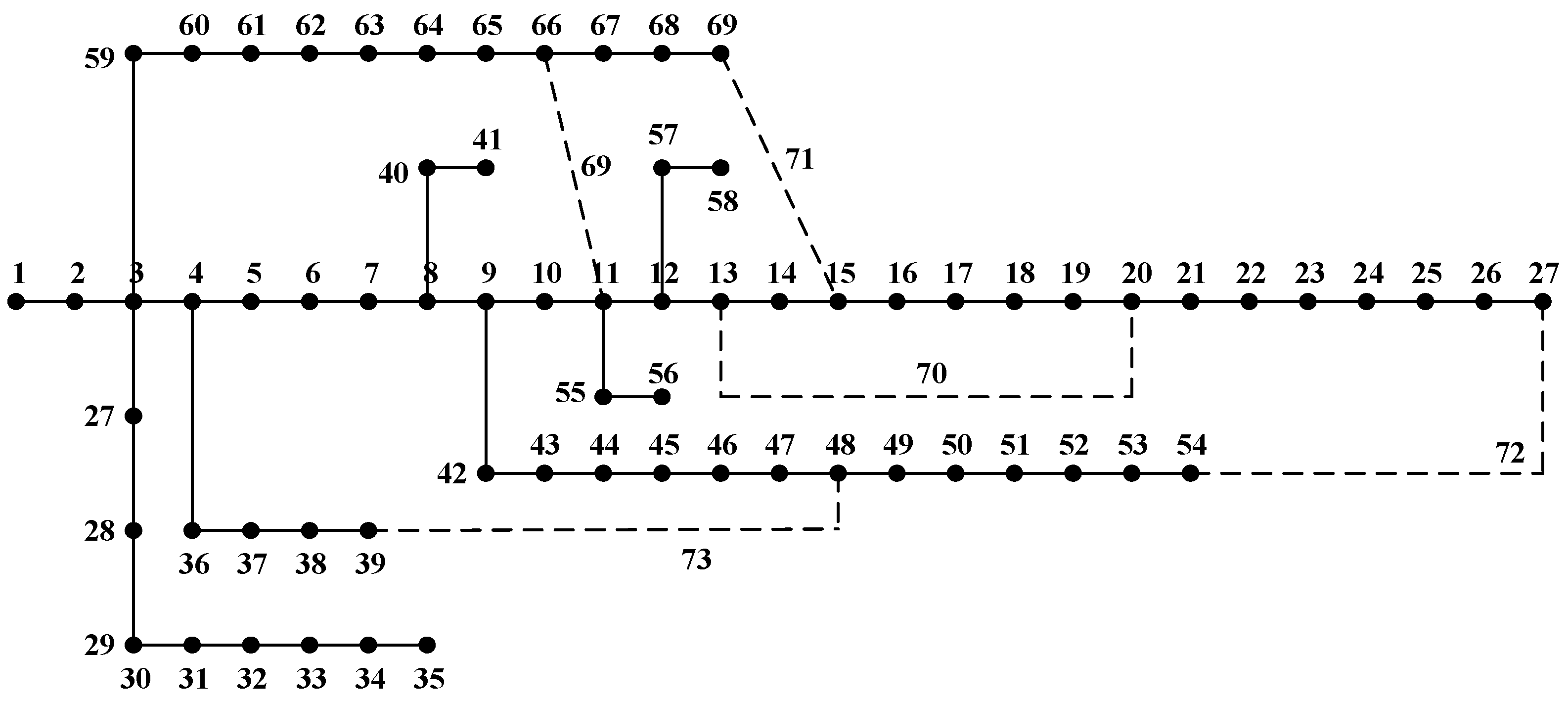
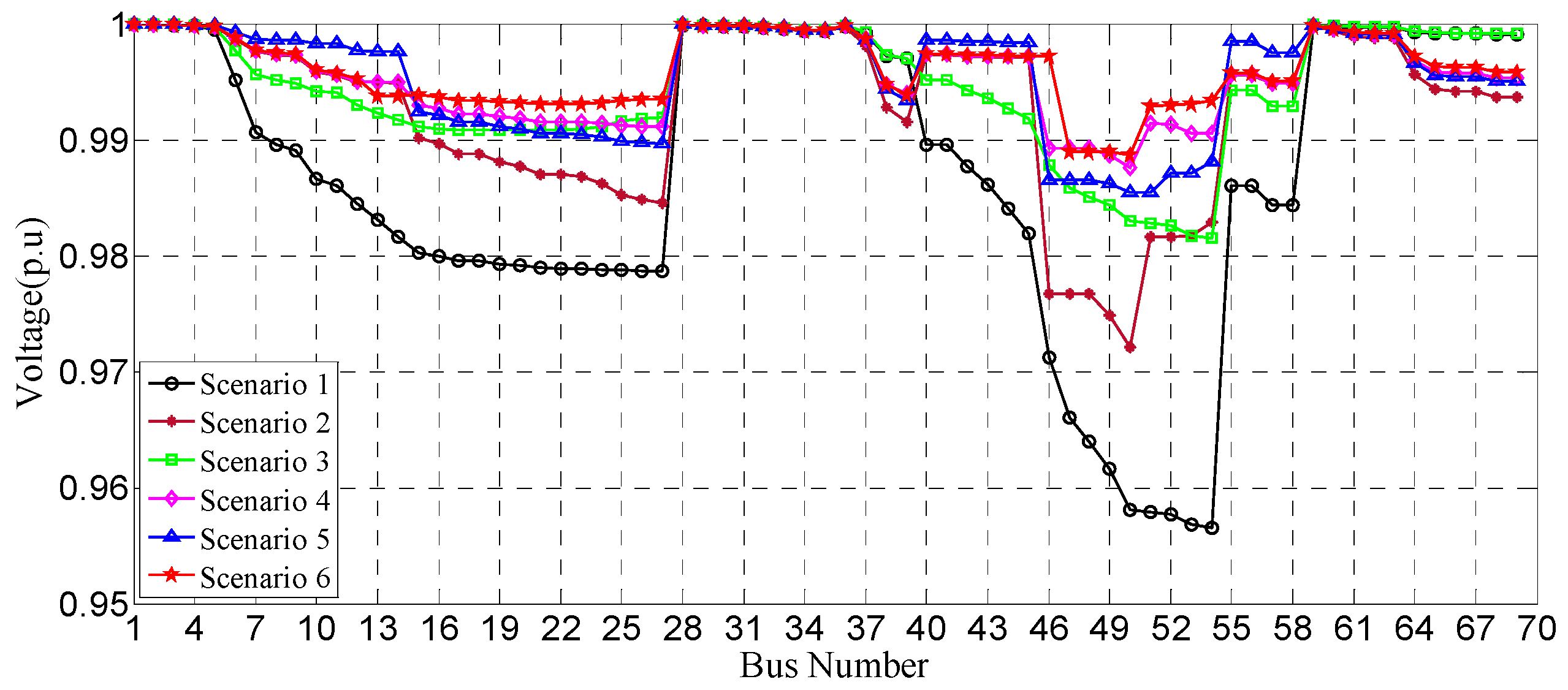
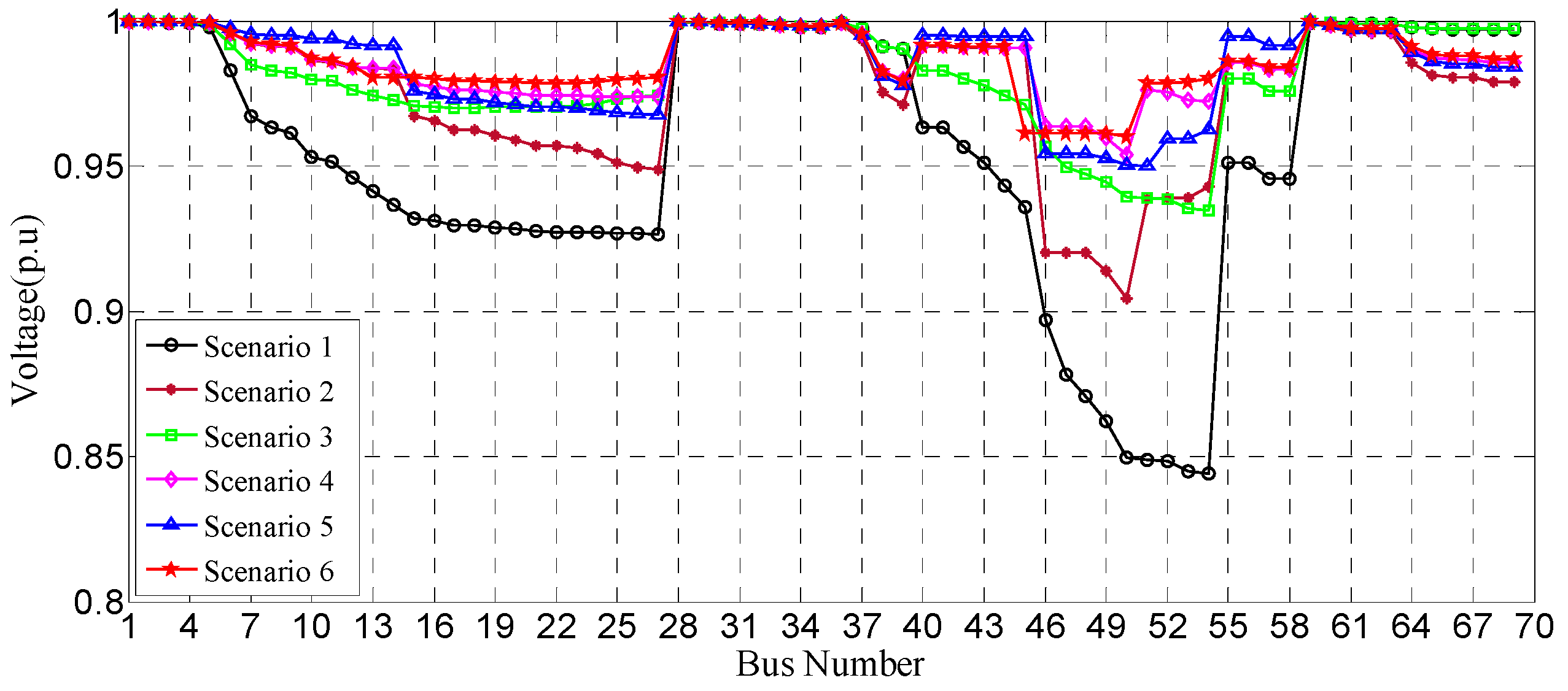
5.2. 69-Bus Test System
6. Conclusions
Author Contributions
Funding
Data Availability Statement
Acknowledgments
Conflicts of Interest
Appendix A

| Scenario | Item | Load Level | ||
|---|---|---|---|---|
| Light (0.5) | Nominal (1.0) | Heavy (1.6) | ||
| Base Case (Scenario 1) | Switches Opened | 33, 34, 35, 36, 37 | 33, 34, 35, 36, 37 | 33, 34, 35, 36, 37 |
| Power Loss (kW) | 47.0644 | 202.6471 | 575.2623 | |
| Minimum Voltage (p.u) | 0.9584 | 0.9133 | 0.8532 | |
| Only Reconfiguration (Scenario 2) | Switches Opened | 7, 14, 9, 32, 37 | 7, 14, 9, 32, 37 | 7, 14, 9, 32, 37 |
| Power Loss (kW) | 33.2513 | 139.7431 | 380.2175 | |
| Minimum Voltage (p.u) | 0.9698 | 0.9378 | 0.8967 | |
| Loss Reduction (%) | 29.35 | 31.04 | 33.91 | |
| Only DG Installation (Scenario 3) | Switches Opened | 33, 34, 35, 36, 37 | 33, 34, 35, 36, 37 | 33, 34, 35, 36, 37 |
| Size of DG (MW) (Candidate Bus) | 0.3375 [bus 16] 0.1079 [bus 18] 0.5826 [bus 31] | 0.6781 [bus 16] 0.2170 [bus 18] 1.1650 [bus 31] | 1.0850 [bus 16] 0.3440 [bus 18] 1.9286 [bus 31] | |
| Power Loss (kW) | 22.2786 | 92.2000 | 247.5140 | |
| Minimum Voltage (p.u) | 0.9873 | 0.9738 | 0.9580 | |
| Loss Reduction (%) | 52.66 | 54.50 | 56.97 | |
| DG Installation after Reconfiguration (Scenario 4) | Switches Opened | 7, 14, 9, 32, 37 | 7, 14, 9, 32, 37 | 7, 14, 9, 32, 37 |
| Size of DG (MW) (Candidate Bus) | 0.0936 [bus 18] 0.3380 [bus 30] 0.1756 [bus 32] | 0.1798 [bus 18] 0.6786 [bus 30] 0.3536 [bus 32] | 0.2725 [bus 18] 1.0837 [bus 30] 0.5526 [bus 32] | |
| Power Loss (kW) | 20.6288 | 85.4004 | 228.6926 | |
| Minimum Voltage (p.u) | 0.9805 | 0.9599 | 0.9333 | |
| Loss Reduction (%) | 56.17 | 57.86 | 60.25 | |
| Reconfiguration after DG Installation (Scenario 5) | Switches Opened | 7, 12, 10, 32, 28 | 7, 12, 10, 32, 28 | 7, 12, 10, 32, 28 |
| Size of DG (MW) (Candidate Bus) | 0.3375 [bus 16] 0.1079 [bus 18] 0.5826 [bus 31] | 0.6781 [bus 16] 0.2170 [bus 18] 1.1650 [bus 31] | 1.0850 [bus 16] 0.3440 [bus 18] 1.9286 [bus 31] | |
| Power Loss (kW) | 16.5002 | 67.9401 | 180.4301 | |
| Minimum Voltage (p.u) | 0.9876 | 0.9747 | 0.9597 | |
| Loss Reduction (%) | 64.94 | 66.47 | 68.64 | |
| Bi-level Optimization Model (Scenario 6) | Switches Opened | 7, 12, 10, 32, 27 | 7, 13, 10, 32, 27 | 7, 13, 10, 32, 26 |
| Size of DG (MW) (Candidate Bus) | 0.3619 [bus 17] 0.4125 [bus 30] 0.3314 [bus 31] | 0.6825 [bus 17] 0.7927 [bus 30] 0.6920 [bus 31] | 1.1112 [bus 17] 1.4301 [bus 30] 1.2312 [bus 31] | |
| Power Loss (kW) | 15.9349 | 65.4468 | 177.6714 | |
| Minimum Voltage (p.u) | 0.9881 | 0.9776 | 0.9642 | |
| Loss Reduction (%) | 66.14 | 67.70 | 69.11 | |
| Scenario | Item | Method Comparison | ||
|---|---|---|---|---|
| The Proposed Method | MPGSA (30) | HAS (21) | ||
| Base Case (Scenario 1) | Switches Opened | 33, 34, 35, 36, 37 | 33, 34, 35, 36, 37 | 33, 34, 35, 36, 37 |
| Power Loss (kW) | 202.6471 | 202.67 | 202.67 | |
| Minimum Voltage (p.u) | 0.9133 | 0.9052 | 0.9131 | |
| Only Reconfiguration (Scenario 2) | Switches Opened | 7, 14, 9, 32, 37 | 7, 14, 9, 32, 37 | 7, 14, 9, 32, 37 |
| Power Loss (kW) | 139.7431 | 139.5 | 138.06 | |
| Minimum Voltage (p.u) | 0.9378 | 0.9343 | 0.9342 | |
| Loss Reduction (%) | 31.04 | 31.17 | 31.88 | |
| Only DG Installation (Scenario 3) | Switches Opened | 33, 34, 35, 36, 37 | 33, 34, 35, 36, 37 | 33, 34, 35, 36, 37 |
| Size of DG (MW) (Candidate Bus) | 0.6781 [bus 16] 0.2170 [bus 18] 1.1650 [bus 31] | 0.1058 [bus 17] 0.5900 [bus 18] 1.0812 [bus 31] | 0.5724 [bus 17] 0.1070 [bus 18] 1.0462 [bus 33] | |
| Power Loss (kW) | 92.2000 | 95.42 | 96.76 | |
| Minimum Voltage (p.u) | 0.9738 | 0.9585 | 0.9670 | |
| Loss Reduction (%) | 54.50 | 52.92 | 52.26 | |
| DG Installation after Reconfiguration (Scenario 4) | Switches Opened | 7, 14, 9, 32, 37 | 7, 9, 13, 32, 37 | 7, 14, 9, 32, 37 |
| Size of DG (MW) (Candidate Bus) | 0.1798 [bus 18] 0.6786 [bus 30] 0.3536 [bus 32] | 0.2469 [bus 30] 0.1795 [bus 31] 0.6645 [bus 32] | 0.6612 [bus 30] 0.1611 [bus 31] 0.2686 [bus 32] | |
| Power Loss (kW) | 85.4004 | 92.87 | 97.13 | |
| Minimum Voltage (p.u) | 0.9599 | 0.9482 | 0.9479 | |
| Loss Reduction (%) | 57.86 | 54.18 | 52.07 | |
| Reconfiguration after DG Installation (Scenario 5) | Switches Opened | 7, 12, 10, 32, 28 | - | - |
| Size of DG (MW) (Candidate Bus) | 0.6781 [bus 16] 0.2170 [bus 18] 1.1650 [bus 31] | - - - | - - - | |
| Power Loss (kW) | 67.9401 | - | - | |
| Minimum Voltage (p.u) | 0.9747 | - | - | |
| Loss Reduction (%) | 66.47 | - | - | |
| Scenario 6 | Switches Opened | 7, 13, 10, 32, 27 | 7, 14, 10, 28, 31 | 7, 14, 10, 28, 32 |
| Size of DG (MW) (Candidate Bus) | 0.6825 [bus 17] 0.7927 [bus 30] 0.6920 [bus 31] | 0.6311 [bus 18] 0.5568 [bus 32] 0.5986 [bus 33] | 0.5586 [bus 31] 0.5258 [bus 32] 0.5840 [bus 33] | |
| Power Loss (kW) | 65.4468 | 72.23 | 73.05 | |
| Minimum Voltage (p.u) | 0.9776 | 0.9724 | 0.9700 | |
| Loss Reduction (%) | 67.70 | 64.36 | 63.59 | |
| Scenario | Item | Load Level | ||
|---|---|---|---|---|
| Light (0.5) | Nominal (1.0) | Heavy (1.6) | ||
| Base Case (Scenario 1) | Switches Opened | 69, 70, 71, 72, 73 | 69, 70, 71, 72, 73 | 69, 70, 71, 72, 73 |
| Power Loss (kW) | 51.9403 | 226.4735 | 656.9548 | |
| Minimum Voltage (p.u) | 0.9566 | 0.9089 | 0.8440 | |
| Only Reconfiguration (Scenario 2) | Switches Opened | 69, 70, 14, 50, 45 | 69, 70, 14, 50, 44 | 69, 70, 14, 50, 45 |
| Power Loss (kW) | 24.0431 | 100.9662 | 275.8305 | |
| Minimum Voltage (p.u) | 0.9721 | 0.9425 | 0.9044 | |
| Loss Reduction (%) | 53.71 | 55.42 | 58.01 | |
| Only DG Installation (Scenario 3) | Switches Opened | 69, 70, 71, 72, 73 | 69, 70, 71, 72, 73 | 69, 70, 71, 72, 73 |
| Size of DG (MW) (Candidate Bus) | 0.1156 [bus 27] 0.6398 [bus 50] 0.2180 [bus 55] | 0.2606 [bus 27] 1.3796 [bus 50] 0.4686 [bus 55] | 0.4155 [bus 27] 1.9835 [bus 50] 0.6520 [bus 55] | |
| Power Loss (kW) | 19.4053 | 76.4004 | 218.4006 | |
| Minimum Voltage (p.u) | 0.9815 | 0.9659 | 0.9346 | |
| Loss Reduction (%) | 62.64 | 66.27 | 66.76 | |
| DG Installation after Reconfiguration (Scenario 4) | Switches Opened | 69, 70, 14, 50, 45 | 69, 70, 14, 50, 44 | 69, 70, 14, 50, 45 |
| Size of DG (MW) (Candidate Bus) | 0.2560 [bus 48] 0.5260 [bus 50] 0.1809 [bus 51] | 1.1316 [bus 48] 0.5424 [bus 50] 0.3610 [bus 51] | 1.5148 [bus 48] 0.9589 [bus 50] 0.6570 [bus 51] | |
| Power Loss (kW) | 10.0542 | 44.1955 | 113.2081 | |
| Minimum Voltage (p.u) | 0.9876 | 0.9736 | 0.9540 | |
| Loss Reduction (%) | 80.64 | 80.49 | 82.77 | |
| Reconfiguration after DG Installation (Scenario 5) | Switches Opened | 69, 70, 14, 51, 45 | 69, 70, 14, 52, 45 | 69, 70, 14, 51, 45 |
| Size of DG (MW) (Candidate Bus) | 0.1156 [bus 27] 0.6398 [bus 50] 0.2180 [bus 55] | 0.2606 [bus 27] 1.3796 [bus 50] 0.4686 [bus 55] | 0.4155 [bus 27] 1.9835 [bus 50] 0.6520 [bus 55] | |
| Power Loss (kW) | 9.9789 | 39.6613 | 107.9193 | |
| Minimum Voltage (p.u) | 0.9854 | 0.9726 | 0.9502 | |
| Loss Reduction (%) | 80.79 | 82.49 | 83.57 | |
| Bi-level Optimization Model (Scenario 6) | Switches Opened | 69, 70, 12, 50, 46 | 69, 70, 12, 50, 46 | 69, 70, 12, 50, 44 |
| Size of DG (MW) (Candidate Bus) | 0.7650 [bus 50] 0.1296 [bus 53] 0.1236 [bus 54] | 1.5193 [bus 50] 0.2536 [bus 53] 0.2680 [bus 54] | 2.3369 [bus 50] 0.3551 [bus 53] 0.5054 [bus 54] | |
| Power Loss (kW) | 9.6358 | 39.2642 | 102.8482 | |
| Minimum Voltage (p.u) | 0.9887 | 0.9768 | 0.9600 | |
| Loss Reduction (%) | 81.45 | 82.66 | 84.34 | |
| Scenario | Item | Method Comparison | ||
|---|---|---|---|---|
| Proposed Method | GA | RGA | ||
| Scenario 2 | Switches Opened | 69, 70, 14, 50, 44 | 69, 18, 13, 56, 61 | 69, 17, 13, 55, 61 |
| Power Loss (kW) | 100.9662 | 99.35 | 100.28 | |
| Minimum Voltage (p.u) | 0.9425 | 0.9428 | 0.9428 | |
| Loss Reduction (%) | 55.42 | 55.85 | 55.42 | |
| Scenario 3 | Switches Opened | 69, 70, 71, 72, 73 | 69, 70, 71, 72, 73 | 69, 70, 71, 72, 73 |
| Size of DG (MW) | 2.1088 | 1.7732 | 1.7868 | |
| Power Loss (kW) | 76.4004 | 86.77 | 87.65 | |
| Minimum Voltage (p.u) | 0.9659 | 0.9677 | 0.9678 | |
| Loss Reduction (%) | 66.27 | 61.43 | 61.04 | |
| Scenario 4 | Switches Opened | 69, 70, 14, 50, 44 | 69, 18, 13, 56, 61 | 69, 17, 13, 55, 61 |
| Size of DG (MW) | 2.0350 | 1.8448 | 1.6396 | |
| Power Loss (kW) | 44.1955 | 51.30 | 52.34 | |
| Minimum Voltage (p.u) | 0.9736 | 0.9619 | 0.9611 | |
| Loss Reduction (%) | 80.49 | 77.20 | 76.73 | |
| Scenario 6 | Switches Opened | 69, 70, 12, 50, 46 | 69, 17, 13, 58, 61 | 10, 16, 14, 55, 62 |
| Size of DG (MW) | 2.0409 | 1.8718 | 2.0654 | |
| Power Loss (kW) | 39.2642 | 40.30 | 44.23 | |
| Minimum Voltage (p.u) | 0.9768 | 0.9736 | 0.9742 | |
| Loss Reduction (%) | 82.66 | 82.08 | 80.32 | |
References
- Jenkins, N.; Ekanayake, J.B.; Strbac, G. Distributed Generation; The Institution of Engineering and Technology: London, UK, 2010. [Google Scholar]
- Su, H. Sitting and Sizing of Distributed Generation Based on Improved Simulated Annealing Particle Swarm Optimization. Environ. Sci. Pollut. Res. 2019, 26, 17927–17938. [Google Scholar] [CrossRef] [PubMed]
- Awerbuch, S.; Preston, A. The Virtual Utility: Accounting, Technology & Competitive Aspects of the Emerging Industry; Springer: Berlin/Heidelberg, Germany, 1997. [Google Scholar]
- Chen, C.; Li, N.; Zhong, P.; Zeng, M. Review of virtual power plant technology abroad and enlightenment to China. Power Syst. Technol. 2009, 37, 2258–2263. [Google Scholar]
- Yu, J.; Zhang, F. Distribution network reconfiguration based on improved immune genetic algorithm. Power Syst. Technol. 2009, 33, 100–105. [Google Scholar]
- Wang, J.; Lv, L.; Liu JHu, C.; Zhu, Y. Reconfiguration of distribution network containing distribution generation units based on improved layered forward-backward sweep method. Power Syst. Technol. 2010, 34, 60–64. [Google Scholar] [CrossRef]
- He, Y.; Peng, J.W.; Mao, L. Scenario model and algorithm for the reconfiguration of distribution network with wind power generators. Proc. CSEE 2010, 30, 12–18. [Google Scholar]
- Tian, H.; Lv, L.; Gao, H.; Li, M.; Wang, G.; Cheng, S.; Zhu, X. Dynamic reconfiguration of distribution network considering power grid operation characteristic. Power Syst. Prot. Control 2015, 43, 9–14. [Google Scholar]
- Behdad, A.; Hooshmand, R.; Gholipour, E. Decreasing activity cost of a distribution system company by reconfiguration and power generation control of DGs based on shuffled frog leaping algorithm. Electr. Power Syst. Res. 2014, 61, 48–55. [Google Scholar]
- Chen, D.; Zhang, X. Distribution network reconfiguration of distributed generation based on amopso algorithm. Acta Energ. Solaris Sin. 2017, 38, 2195–2203. [Google Scholar]
- Li, Z.; Chen, X.; Yu, K.; Liu, H.; Zhao, B. Hybrid particle swarm optimization for distribution network reconfiguration. Proc. CSEE 2008, 28, 35–41. [Google Scholar]
- Xiang, X.; Liao, D.; Xiang, N.; Wang, B. Distribution network reconfiguration based on parallel Tabu search algorithm. Power Syst. Technol. 2012, 36, 100–105. [Google Scholar]
- Xue, Y.; Wu, X.; Wei, W. Distribution network reconfiguration with BPSO based on combination of loop group search and individual loop replacement. Power Syst. Technol. 2016, 40, 263–269. [Google Scholar]
- Ji, X.; Liu, Q.; Yu, Y. Two-level reconfiguration algorithm based on power moment and neighbourhood searching for distribution network. Electr. Power Autom. Equip. 2017, 37, 28–34. [Google Scholar]
- Nasiraghdam, H.; Jadid, S. Optimal hybrid PV/WT/FC sizing and distribution system reconfiguration using multi-objective artificial bee colony (MOABC) algorithm. Sol. Energy 2012, 86, 3057–3071. [Google Scholar] [CrossRef]
- Rosseti, G.; de Oliveira, E.; de Oliveira, L.; Silva, J.; Peres, W. Optimal allocation of distributed generation with reconfiguration in electric distribution systems. Electr. Power Syst. Res. 2013, 103, 178–183. [Google Scholar] [CrossRef]
- Mohamed, I.A.; Kowsalya, M.; Kothari, D. A novel integration technique for optimal network reconfiguration and distributed generation placement in power distribution networks. Elect. Power Energy Syst. 2014, 63, 461–472. [Google Scholar] [CrossRef]
- Bayat, A.; Bagheri, A.; Noroozian, R. Optimal siting and sizing of distributed generation accompanied by reconfiguration of distribution networks for maximum loss reduction by using a new UVDA-based heuristic method. Int. J. Electr. Power Energy Syst. 2016, 77, 360–371. [Google Scholar] [CrossRef]
- Yin, X.; Ye, C.; Ding, Y.; Song, Y. Exploiting Internet Data Centers as Energy Prosumers in Integrated Electricity-Heat System. IEEE Trans. Smart Grid 2023, 14, 167–182. [Google Scholar] [CrossRef]
- Xu, Y.; Liu, Z.; Zhang, C.; Ren, J.; Zhang, Y.; Shen, X. Blockchain-Based Trustworthy Energy Dispatching Approach for High Renewable Energy Penetrated Power Systems. IEEE Internet Things J. 2022, 9, 10036–10047. [Google Scholar] [CrossRef]
- Mansouri, S.A.; Ahmarinejad, A.; Nematbakhsh, E.; Javadi, M.S.; Nezhad, A.E.; Catalao, J.P.S. A Sustainable Framework for Multi-Microgrids Energy Management in Automated Distribution Network by Considering Smart Homes and High Penetration of Renewable Energy Resources. Energy 2022, 245, 123228. [Google Scholar] [CrossRef]
- Li, Y.; Gao, D.W.; Gao, W.; Zhang, H.; Zhou, J. A Distributed Double-Newton Descent Algorithm for Cooperative Energy Management of Multiple Energy Bodies in Energy Internet. IEEE Trans. Ind. Inform. 2021, 17, 5993–6003. [Google Scholar] [CrossRef]
- Ameli, A.; Shahab, B.; Farid, K.; Mahmood, R.H. A multiobjective particle swarm optimization for sizing and placement of DGs from DG Owner’s and distribution company’s viewpoints. IEEE Trans. Power Deliv. 2014, 9, 1831–1840. [Google Scholar] [CrossRef]
- Su, H.; Zhang, Z. Power Flow algorithm for weakly meshed distribution network with distributed generation based on loop-analysis in different load models. J. Electr. Eng. Technol. 2018, 13, 608–619. [Google Scholar]
- Srinivasa, R.; Ravindra, K.; Satisk, K.; Narasimham, S. Power loss minimization in distribution system using network reconfiguration in the presence of distributed generation. IEEE Trans. Power Syst. 2013, 28, 317–325. [Google Scholar]
- Wang, X.; Wei, Z.; Sun, G.; Li, Y.; Zang, H. Multi-objective distribution network reconfiguration considering uncertainties of distributed generation and load. Electr. Power Autom. Equip. 2016, 36, 116–121. [Google Scholar]
- Chen, C.; Wang, F.; Liu, B.; Cao, Y.; Huang, C.; Dong, X. Network reconfiguration based on basic ring matrix and improved harmony search algorithm. Autom. Electr. Power Syst. 2014, 38, 55–60. [Google Scholar]
- Geem, Z.; Kim, J.; Loganathan, G. A new heuristic optimization algorithm: Harmony search. Simulation 2001, 76, 60–68. [Google Scholar] [CrossRef]
- Li, Z. An Adaptive Harmony Search Algorithm for Network Reconfiguration Considering Reliability. Master’s Thesis, Zhejiang University, Hangzhou, China, 2017. [Google Scholar]
- Jiang, Y.; Chen, Z.; Huang, C.; Cao, Y.; Sun, Y.; Jia, T. Distribution network reconfiguration based on heuristic rules and harmony search algorithm. J. Hunan Univ. Nat. Sci. Ed. 2014, 4, 61–67. [Google Scholar]
- Liang, S. Distribution Network Reconfiguration Based on Improved Harmony Search Algorithm. Master’s Thesis, Hunan University, Changsha, China, 2016. [Google Scholar]
- Mistry, K.; Roy, R. Enhancement of loading capacity of distribution system through distributed generator placement considering technoeconomic benefits with load growth. Int. J. Electr. Power Energy Syst. 2014, 54, 505–515. [Google Scholar] [CrossRef]
- Baran, M.; Wu, F. Network reconfiguration in distribution systems for loss reduction and load balancing. IEEE Trans. Power Deliv. 1989, 4, 1401–1409. [Google Scholar] [CrossRef]
- Rajaram, R.; Kumar, S.; Rajasekar, N. Power system reconfiguration in a radial distribution network for reducing losses and to improve voltage profile using modified plant growth simulation algorithm with Distributed Generation (DG). Energy Rep. 2015, 1, 116–122. [Google Scholar] [CrossRef]
- Savier, J.S.; Das, D. Impact of Network Reconfiguration on Loss Allocation of Radial Distribution Systems. IEEE Trans. Power Deliv. 2007, 22, 2473–2480. [Google Scholar] [CrossRef]


| Scenario | Specific Division |
|---|---|
| Scenario 1 | Original state without DGs and reconfiguration |
| Scenario 2 | Only reconfiguration |
| Scenario 3 | Only DG allocation |
| Scenario 4 | DG allocation after reconfiguration |
| Scenario 5 | Reconfiguration after DG allocation |
| Scenario 6 | Dual-layer optimization |
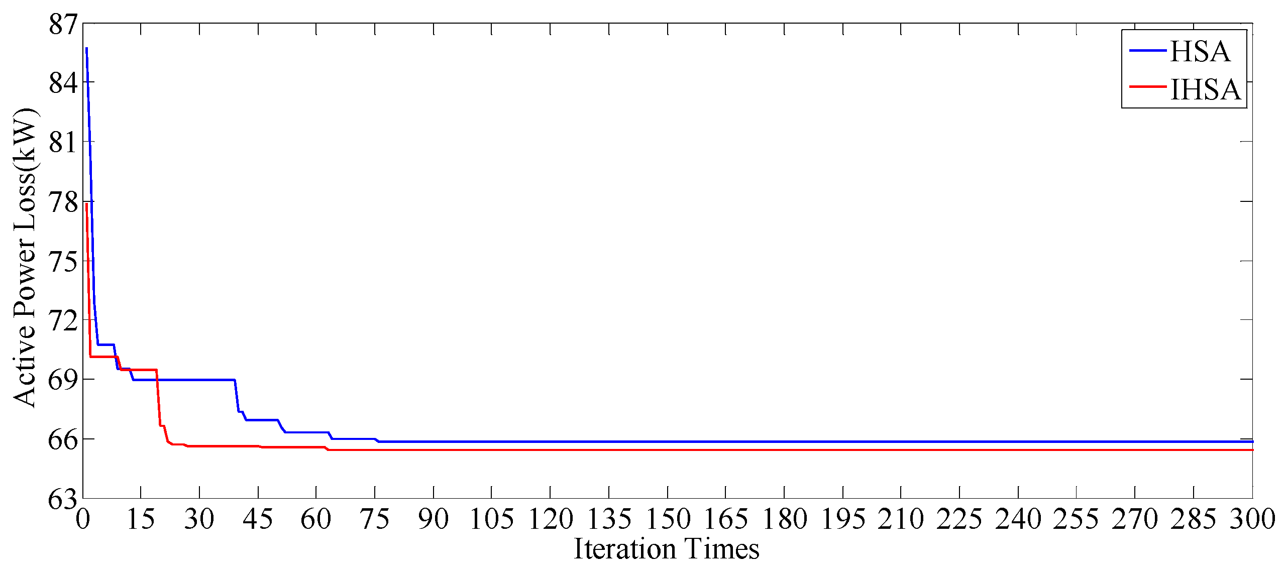
| Algorithm | Reconfiguration Results | Active Power Loss (kW) | The Minimum Voltage (p.u) | Iteration Times |
|---|---|---|---|---|
| HSA | [7 13 10 32 28] | 65.8501 | 0.9721 | 79 |
| IHSA | [7 13 10 32 27] | 65.4468 | 0.9776 | 63 |
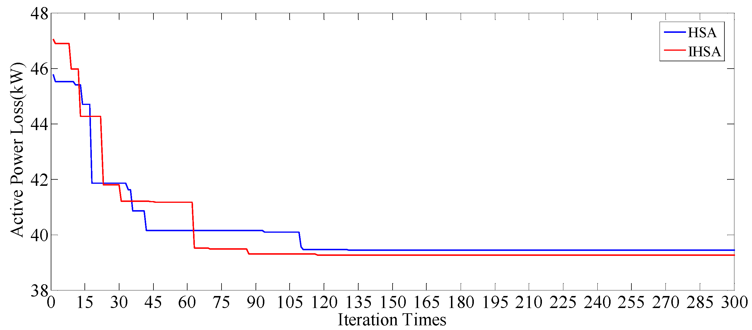
| Algorithm | Reconfiguration Results | Active Power Loss (kW) | The Minimum Voltage (p.u) | Iteration Times |
|---|---|---|---|---|
| HSA | [69 70 12 50 47] | 39.4354 | 0.9747 | 131 |
| IHSA | [69 70 12 50 44] | 39.2642 | 0.9768 | 117 |
Disclaimer/Publisher’s Note: The statements, opinions and data contained in all publications are solely those of the individual author(s) and contributor(s) and not of MDPI and/or the editor(s). MDPI and/or the editor(s) disclaim responsibility for any injury to people or property resulting from any ideas, methods, instructions or products referred to in the content. |
© 2023 by the authors. Licensee MDPI, Basel, Switzerland. This article is an open access article distributed under the terms and conditions of the Creative Commons Attribution (CC BY) license (https://creativecommons.org/licenses/by/4.0/).
Share and Cite
Su, H.; Wang, X.; Ding, Z. Bi-Level Optimization Model for DERs Dispatch Based on an Improved Harmony Searching Algorithm in a Smart Grid. Electronics 2023, 12, 4515. https://doi.org/10.3390/electronics12214515
Su H, Wang X, Ding Z. Bi-Level Optimization Model for DERs Dispatch Based on an Improved Harmony Searching Algorithm in a Smart Grid. Electronics. 2023; 12(21):4515. https://doi.org/10.3390/electronics12214515
Chicago/Turabian StyleSu, Hongsheng, Xingsheng Wang, and Zonghao Ding. 2023. "Bi-Level Optimization Model for DERs Dispatch Based on an Improved Harmony Searching Algorithm in a Smart Grid" Electronics 12, no. 21: 4515. https://doi.org/10.3390/electronics12214515
APA StyleSu, H., Wang, X., & Ding, Z. (2023). Bi-Level Optimization Model for DERs Dispatch Based on an Improved Harmony Searching Algorithm in a Smart Grid. Electronics, 12(21), 4515. https://doi.org/10.3390/electronics12214515