Stereo Matching Algorithm of Multi-Feature Fusion Based on Improved Census Transform

Abstract

This article proposes an improved stereo matching algorithm in order to address the issue that the conventional Census transform is overly dependent on the center pixel of the window, which makes the algorithm susceptible to noise interference and results in low matching accuracy in regions with weak texture and complex texture. In the cost calculation stage, the noise threshold is set utilizing the absolute difference detection approach, and pixels that exceed the threshold are replaced with the mean gray values of the neighboring pixels in the 3 × 3 window. This stage also includes the introduction of the gradient cost, which is coupled with the edge and feature point information to provide the final matching cost. The cross approach is employed to build the adaptive support domain and aggregate the costs during the cost aggregation stage. The disparity is finally calculated using the WTA technique, and a multi-step refinement process is employed to produce the final disparity map. The experiments demonstrate that the proposed algorithm has good anti-noise performance. Compared with other improved algorithms or composite algorithms, the average matching rate of the four standard images on the Middlebury test platform is 5.53%, which is higher than the remaining algorithms, indicating that the matching accuracy is high. The proposed algorithm provides ideas for subsequent improved algorithms.

1. Introduction

Stereo matching seeks to identify analogous pixels from images captured from varying perspectives. The process involves computing the disparity between corresponding pixels to obtain depth information. Stereo matching technology is extensively adopted in autonomous driving, target tracking and three-dimensional reconstruction [1,2,3].

The accuracy of matching and real-time performance of stereo matching algorithms have significantly increased as a result of extensive recent research by relevant academics both domestically and internationally [4]. In their summary of the matching process, Scharstein et al. [5] categorized the matching process into four stages: cost calculation, cost aggregation, disparity calculation and disparity refinement. They also classified the standard stereo matching algorithm into global stereo matching algorithm and local stereo matching algorithm [6,7]. The global algorithm obtains the optimal disparity value by minimizing the energy function. There are mainly global algorithms based on dynamic programming [8], belief propagation [9] and graph cut [10]. The global stereo matching algorithm has a good matching effect, but it is difficult to apply to applications with high real-time requirements due to its high computational complexity and being time-consuming. The local stereo matching algorithm uses the pixel information in the neighborhood of the point to be matched to calculate the cost. The advantage is that the algorithm has low complexity and good real-time performance. Sum of absolute difference (SAD) [11], relative gradient [12], normalized cross correlation (NCC) [13] and Census transform (CT) [14] are commonly used to calculate the matching cost of two pixels. Among them, Census transform typically takes the left image as the reference image, extracts the gray information within the neighborhood window of the center point, and uses this as a measure to find the corresponding points in the right image. It is a classical local stereo matching algorithm [15]. Now, Census transform is widely applied in real-time applications involving 3D measurements because of its fast-running speed, speedy performance, resilience to variations in illumination and ease of implementation. Nevertheless, the algorithm also presents limitations: (1) Overly dependent on central pixels; (2) vulnerability to noise; (3) poor matching performance in intricate textures, multi-edged regions and low-texture areas [16].

In view of the above-mentioned limitations, Liu et al. [17] have proposed a matching cost function that effectively combines enhanced matching cost with image gradient and improved matching cost with Census transform. The experiments conducted showed that the matching cost function is immune to radiation changes and low-texture regions. Additionally, Zin et al. [18] have proposed a Graph Cut stereo matching algorithm that is based on Census transform. This algorithm has been improved for better performance. The similarity measure in the data term of the energy function is determined by the Hamming distance between the corresponding pixels in the left and right images after the introduction of Census transform. This effectively reduces any reliance on pixel values. Applying this method, our stereo matching experiments are executed on both the standard images of the Middlebury stereo benchmark and real scene images, demonstrating that our algorithm is not only robust but also achieves superior results in regions of weak or repeated texture. Hou et al. [19] proposed a stereo matching algorithm which utilizes the Census transform and texture filtering. The matching cost is computed using the weighted Census transform circular template, reflecting the influence of the distance between neighboring pixels and the target pixels and expanding the perception range of the target pixels. Mei et al. [20] proposed an AD-Census stereo matching algorithm with fusion cost that ensures high matching accuracy in high texture regions and robustness to external factors, such as illumination. Chen et al. [21] proposed a stereo matching algorithm that uses the HSV color space and an enhanced Census transform. Lee et al. [22] proposed the Star-Census transform, which compares pixel brightness at a certain distance along a symmetrical pattern within the matching window. The experiment results suggest that the proposed algorithm outperforms previous CT algorithms.

In stereo matching, two homonymous points often have similar texture patterns, brightness levels, etc. Therefore, multi-feature fusion is one of the methods to solve this problem. The method of multi-feature fusion has been widely used in many fields because of its high adaptability. Liu, C et al. [23] applied the method of multi-feature fusion to the medical vision model, fused the features from medical images and clinical texts, and proposed an M-FLAG algorithm (Medical vision-language pre-training with Frozen language models and Latent spAce Geometry optimization). The experimental results show that the algorithm has achieved excellent performance in the segmentation task. Cheng, S et al. [24] studied the integration of data assimilation (DA), uncertainty quantification (UQ) and machine learning (ML) techniques to solve some key challenges in high-dimensional dynamic systems. Therefore, this paper proposes an enhanced Census-transform-based multi-feature fusion stereo matching algorithm, which avoids the dependence on the center pixel and improves the resistance to noise. The gradient is fused with the edge and feature point information introduced at the same time to generate the final matching cost. The cross-domain cost aggregation method is used to calculate the aggregation cost. Ultimately, the WTA [25] method and multi-step refining are used to produce the final disparity map.

This paper is organized as follows: Section 2 discusses the fundamentals of the traditional Census algorithm, its drawbacks and improvements made in response to those drawbacks. The comparison and results of traditional algorithms and improved algorithms are presented in Section 3. Finally, the paper is concluded and analyzed in Section 4.

2. Principle and Method

2.1. Matching Cost Calculation

The matching cost is a crucial aspect in stereo matching. It is utilized for evaluating the similarity of the corresponding pixels in two images taken by the camera from different perspectives in the same scene and typically influenced by factors such as lighting and background noise [26].

2.1.1. Traditional Matching Cost Calculation

The conventional Census algorithm traverses the image’s pixels in a rectangular window, chooses the gray value of the window’s center point as the reference value, and compares the gray values of each pixel to the reference value. The Boolean value obtained from the comparison is mapped into a bit string and the value of the bit string is used as the Census transformation value of the central pixel [27]. Normally, the process of transformation can be given as

$$C\left(p\right)=\otimes \xi [I\left(p\right),I\left(q\right)],q\in \mathsf{\Omega }$$

(1)

where $\otimes$ represents the bit-wise catenation, $I\left(p\right)$ is the gray value of the central pixel p in the window, $I\left(q\right)$ is the gray value of another point q in the same window. In Equation (1), the traditional Census auxiliary function for $I\left(p\right)$ and $I\left(q\right)$ is given as

$$\xi \left[I(p),I(q)\right]=\left\{\begin{array}{cc}0,& I(p)\le I(q)\\ 1,& I(p)\ge I(q)\end{array}\right.,q\in \mathsf{\Omega }$$

(2)

where $\mathsf{\Omega }$ comprises all the other points in the support window besides the central point; $\xi \left[I(p),I(q)\right]$ is the Census transform value.

According to Equation (1), Census transform is performed on the left and the right image in a certain disparity range, and two-bit strings are obtained. The Hamming distance of two-bit strings is compared bit by bit. The computation of the similarity between $I\left(p\right)$ and $I\left(q\right)$ by Hamming is given as

$$C(p,d)=Hamming\left[C_l(p),C_r(p-d)\right],d\in [d_{\min },d_{\max }]$$

(3)

where $C\left(p,d\right)$ is the matching cost; when the parallax is d, $C_l(p)$ is the bit string of the left image and $C_{\mathrm{r}}(p-d)$ is the bit string of the right image. $d_{\max }$ and $d_{\min }$ are the maximum and minimum values of the disparity range, respectively.

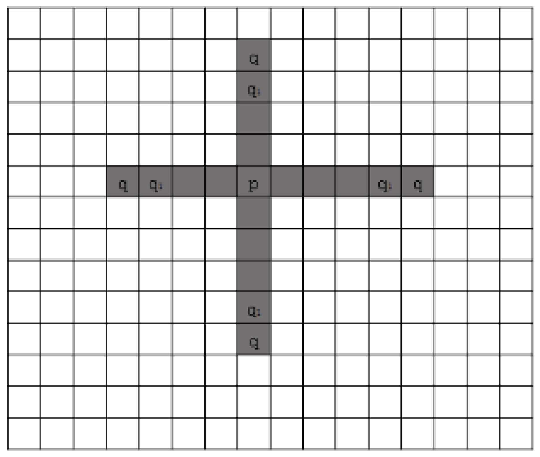
2.1.2. Improved Matching Cost Calculation

When choosing the reference value information, the traditional Census algorithm just takes the gray value of the window’s center point into consideration. The result is overly dependent on the center point, leading to sensitivity to noise and being easy to cause mismatch. To solve this problem, MA et al. [28] replaced the gray value of the center pixel with the mean gray value of the neighborhood pixels in the support window. Although the dependence on the center pixel is reduced, the reliability of the obtained reference value becomes worse. This paper presents a matching cost algorithm rooted in multi-feature fusion in light of the aforementioned issues. Figure 1 is the flow chart of the algorithm.

The Rank-Ordered Absolute Differences (ROAD) [29] is used to detect whether the center point is a noise point. The principle is as follows: define p as the center pixel and ${\mathsf{\Omega }}_{3\times 3}$ as the set of pixels except the center point in the 3 × 3 window. $d_{p,q}$ is the absolute value of the gray value difference between the center pixel p and the neighborhood pixel q and is given as

$$d_{p,q}=\left|I(p)-I(q)\right|,q\in {\mathsf{\Omega }}_{3\times 3}$$

(4)

Then, all the $d_{p,q}$ values in the window are arranged in ascending order and defined as

$$ROA{D}_m(x)={\displaystyle \sum _{i=1}^m{r}_i(x)}$$

(5)

In the above equation, 2 ≤ m ≤ 7, $r(x)$ is the set of d_{p, q}, and $r_i(x)$ denotes the value at the i-th position in the ascending order.

The edge pixels and impulse noise pixels of the Lena image are contrasted in Figure 2. By comparing the two images, it can be noticed that the neighborhood around the edge pixel has almost the same intensity, which means that its ROAD value is very low.

The internal area and edge of the image are continuous, so when the ROAD value is low, the gray values of the center pixels are similar to those of the neighboring pixels. However, when the center point is affected by noise, it differs significantly from most or all of the neighboring pixels in terms of gray value, resulting in a higher ROAD value. The value of ROAD₄ represents the similarity between half of the pixels in the 3 × 3 window and the center pixel, which is the best choice to judge the noise. Therefore, this paper utilizes the values of ROAD₄ to determine whether the center point of the support window is a noise point.

During the cost calculation, a threshold T_noise is established. The center pixel will be modified when the threshold is surpassed. By replacing gray value of the center pixel with the average gray value of the neighboring pixels, the mismatch rate can be drastically reduced. However, the window selected according to the center point is typically larger in the real calculation cost, and numerous picture edges or multiple noise locations are more likely to appear in the window. In most cases, the points in the 3 × 3 window have outstanding continuity and the likelihood of multiple noise points is low. Therefore, this paper employs the average gray value of the 3 $\times$ 3 window pixels except the center pixels as the gray value of the reference. The gray value of the reference point I(p) of the transformation is given as

$$I\left(p\right)=\left\{\begin{array}{cc}I(p),& ROA{D}_4\le T_{noise}\\ \frac{1}{N-1}{\displaystyle \sum _{q\in N(p)}I(q)}& ROA{D}_4\ge T_{noise}\end{array}\right.$$

(6)

where $N\left(p\right)$ is the set of all domain points except the central pixel in the 3 × 3 window.

Figure 3 depicts the transformation and comparison procedure. The Census transform without noise is shown in the first part, followed by the conventional Census transform with noise added, and finally, the improved Census transform results with noise added. Even though the center point is disturbed, the bit string obtained by the transformation is less affected. Therefore, this algorithm can reduce the dependence on the center point. At the same time, the judgment of noise is added to improve the reliability of the reference value of the support window in the Census transform.

Although the reliance on the center point is lessened through judgment and adjustment of gray value of the center point, it is still unable to effectively improve the algorithm’s effect in the weakly textured and the repeated textured regions. Therefore, this paper introduces edge and feature point information to improve the precision of the algorithm.

First, Canny edge detection is required to create an initial binary image and then encode it in order to extract rich edge texture information. The specific coding conversion process is given as

$$E(q)=\left\{\begin{array}{cc}1,& I(q)=255\\ 0,& I(q)=0\end{array}\right.,q\in {\mathsf{\Omega }}_{edge}$$

(7)

where $E\left(q\right)$ is the edge binary value obtained from the point q and ${\mathsf{\Omega }}_{edge}$ is the set of neighborhood pixels of q in the edge image.

Then, the Harris corner detection method is employed to obtain the corner points in the image. By setting the distance between the corner points, the feature point set ${\mathsf{\Omega }}_{feature}$ is obtained. Finally, the edge information and corner information are combined to construct the following comparison function:

$$\xi {[I(p),I(q)]}_{edge+feature}=\left\{\begin{array}{cc}11& E(q)=1,q\in {\mathsf{\Omega }}_{feature}\\ 10& E(q)=1,q\notin {\mathsf{\Omega }}_{feature}\\ 01& E(q)=0,q\in {\mathsf{\Omega }}_{feature}\\ 00& E(q)=0,q\notin {\mathsf{\Omega }}_{feature}\end{array}\right.$$

(8)

Taking the 3 × 3 support window as an example, the specific Census transform coding and combination process of edge and feature point information is shown in Figure 4. ‘X‘ is the position where the feature points are distributed in the support window.

After introducing the edge and feature point information, the matching cost is calculated in accordance with Formula (2), and it is linearly fused with the initial cost calculated by the gray scale. The matching cost $C_{\mathrm{weight}}(p,d)$ is given as

$$C_{\mathrm{weight}}(p,d)=\epsilon C_{cen}(p,d)+(1-\epsilon )C_{edge+feature}(p,d)$$

(9)

where $C_{cen}(p,d)$ is the Census matching cost based on gray value information, $C_{edge+feature}(p,d)$ is the matching cost based on edge and feature points, and $\epsilon$ is the control parameter. When $\epsilon$ is 0.5, the weight is linear fusion.

In order to improve the smoothness after edge filtering, this paper combines the enhanced transform with the gradient transform. When calculating the gradient, the gradient value of each pixel in the x and y directions should be taken into consideration. The calculation formula based on gradient transformation can be expressed as

$$C_{Grad}(p,d)=\left|{\nabla }_x{I}_l(p)-{\nabla }_x{I}_r(p-d)\right|+\left|{\nabla }_y{I}_l(p)-{\nabla }_y{I}_r(p-d)\right|$$

(10)

where $\nabla$ is the directional derivative, $I_l(p)$ is the gray value of point p in the left image, and $I_r(p-d)$ is the gray value of point p to be matched in the right image.

The final cost derived from the improved Census algorithm is fused with the gradient cost using normalization, which is expressed as

$$C(p,d)=2-\exp (-\frac{C_{weight}(p,d)}{{\lambda }_1})-\exp (-\frac{C_{Grad}(p,d)}{{\lambda }_2})$$

(11)

where ${\lambda }_1$ and ${\lambda }_2$ are the parameters that affect the cost weight.

2.2. Cost Aggregation

Cost aggregation plays a key role in stereo matching and affects the final disparity map directly. For cost aggregation, this paper employs the adaptive window based on cross intersection in Reference [16]. Firstly, a cross-domain is built for each pixel, which involves extending the point in the four directions and the limitation criteria. The extension is terminated if the restriction conditions are not satisfied. The specific process is shown in Figure 5.

In Figure 5, p is the center point, q is the end point of the pixel cross arm centered on O point, and q₁ is a point behind the point q. The restriction condition is express as

$$\left\{\begin{array}{l}\begin{array}{cc}\underset{i\in \left\{R,G,B\right\}}{\max }\left|I_i(p)-I_i(q)\right|<{\tau }_1& \\ \underset{i\in \left\{R,G,B\right\}}{\max }\left|I_i(p)-I_i(q_1)\right|<{\tau }_2& \\ L_{\max }\left|l\left(p\right)-l\left(q\right)\right|<L_1& \end{array}\\ \underset{i\in \left\{R,G,B\right\}}{\max }\left|I_i(p)-I_i(q)\right|<{\tau }_3,if\begin{array}{c}\end{array}{L}_2<L_{\max }\left|l\left(p\right)-l\left(q\right)\right|<L_1\end{array}\right.$$

(12)

where ${\tau }_1$, ${\tau }_2$ and ${\tau }_3$ are the color thresholds and $L_1$ and $L_2$ are the distance thresholds.

Then, a support window is constructed based on the cross-arm. Each point in the four extended arms is extended vertically and horizontally with the same constraints. However, the support windows may not always be the same. In order to ensure good matching accuracy and matching effect, the intersection of the two support windows is taken as the final support window. The final support window can be observed in Figure 6.

In Figure 6, orange is the support window of point A, green is the support window of point B and grey is the cross-arm. Since the support windows of the two do not intersect, the rightmost part of the support window of point B will be discarded.

The final aggregation cost $C\left(p,d\right)$ is given as

$$C(p,d)=C^{\prime }(x,y,d)=\frac{{\displaystyle \sum _{q\in U(x,y,d)}C(x,y,d)}}{m}$$

(13)

where $U\left(x,y,d\right)$ represents the support window, q represents the pixel point, $C\left(x,y,d\right)$ represents the initial matching cost, $C^{\prime }(x,y,d)$ represents the value obtained after the cost aggregation, and m represents the total number of points in the window.

2.3. Disparity Calculation

The disparity calculation adopts a simple and efficient WTA strategy. First, the initial disparity $D(p)$ is chosen as the disparity value corresponding to the minimal aggregation cost and it can be given as

$$D(p)=\underset{d\in [0,d\max ]}{\arg \min }[C_A(p,d)]$$

(14)

where $d_{\max }$ is the maximum parallax.

Then, a multi-step refinement scheme is adopted for the initial disparity, including left–right consistency detection, iterative support domain voting, abnormal point classification interpolation, sub-pixel refinement and median filtering.

On each point in the initial disparity map, the formula used to detect the consistency on the left and right sides is given as

$$\left|D_L(p)-D_R[p-D_L(p)]\right|\le \delta =1,$$

(15)

where $D_L(p)$ is the value of point p in the left disparity map, $D_R[p-D_L(p)]$ is the value of the corresponding point of point p in the right disparity map, and $\delta$ is the error tolerance. The points that satisfy the validation are marked as valid points, and other points are marked as outliers.

$$\left\{\begin{array}{c}\left|R(p)\right|>{\tau }_n\\ \frac{\left|d_{R(p)}^{}\right|}{\left|R(p)\right|}>{\tau }_r\end{array}\right.$$

(16)

In the above formula, $\left|R(p)\right|$ is the number of points in the support domain $R(p)$ where the point p is located, $\left|d_{R(p)}\right|$ is the number of the votes for the disparity point $d_{R(p)}$ with the highest number of votes in the support domain $R(p)$, and ${\tau }_n,{\tau }_r$ are the thresholds. If the support domain where the outliers are located satisfies condition (16), the value of $d_{R(p)}$ is used instead of the outliers and marked as a valid point. In order to deal with more outliers, this process needs to be iterated repeatedly.

Abnormal point classification and interpolation are used to handle remaining abnormal points. Firstly, the anomalous points are categorized into occlusion points and mismatch points based on the geometric principle. Then, for the occlusion point, replace it with the nearest effective point in its left and right directions; for the mismatched point, find the nearest effective point in its left and right directions, respectively, and replace the mismatched point with the smaller disparity values of these two points.

Finally, sub-pixel refinement and median filtering are applied to the disparity map in order to obtain the ultimate disparity map.

3. Data and Experiments

In order to verify the effectiveness and stability of the proposed algorithm, this paper verifies it on some stereo image pairs of the Middlebury dataset [30,31,32]. The mismatch rate, which is an important criterion in the test, can be expressed as

$$P_{PBM}=\frac{1}{N}{\displaystyle \sum _{(x,y)}\left[\left|d_e(x,y)-d_r(x,y)\right|>{\sigma }_d\right]}$$

(17)

where N is the number of effective pixels in the image region; $d_e(x,y)$ is the disparity map calculated by the stereo matching algorithm; the true disparity map is provided by $d_r(x,y)$ for the dataset; and ${\sigma }_d$ is the disparity threshold, which is taken as 1 in the experiment. When the difference between the disparity value calculated by the stereo matching algorithm and the real disparity value is larger than 1, the pixel is regarded as a mismatched point.

3.1. Anti-Noise Experiment

Firstly, to assess the accuracy of the suggested algorithm under the influence of noise, salt and pepper noise and Gaussian noise, respectively, are added to the four sets of standard test images. The coverage of salt and pepper noise is 2%, 5%, 10% and 15%, and the size of Gaussian noise is 2, 4, 6 and 8 standard deviations. Utilizing the three different algorithms, the initial cost matrix and unoptimized initial disparity map are acquired. Subsequently, the mean error values of the non-occluded area are assessed and compared with that of the MCT [28] and SGM [33] algorithms. The results after experiments are shown in

Table 1. The mismatch rate of different algorithms under two kinds of noise.

Algorithm	No Noise	Salt and Pepper Noise (%)				Gaussian Noise ($\mathit{\sigma }$)
		2	5	10	15	2	4	6	8
MCT	4.31	5.13	6.16	8.81	13.14	5.22	6.58	8.88	11.01
SGM	5.37	6.21	7.75	10.79	17.68	6.81	9.36	12.03	14.97
Proposed algorithm	3.99	4.33	4.87	5.97	7.31	4.67	6.21	7.83	9.92

.

To provide a clearer comparison of the anti-noise capabilities of the three algorithms, an average mismatch rate line chart for the non-occluded area under the influence of salt and pepper and Gaussian noise was created based on the data from Table 1.

The statistical analysis presented in Table 1 and Figure 7 indicates that in the case of non-occluded area and no noise, the MCT algorithm exhibits a close approximation to the proposed algorithm. However, after adding salt and pepper noise, the mismatch rate of MCT and SGM algorithms increases rapidly, which indicates that the two algorithms are more sensitive to the impulse noise. The proposed algorithm, however, performs under the same conditions with a relatively stable and robust performance, making it a better choice. Although the distinction between the proposed method and the other two algorithms is not strikingly apparent for Gaussian noise, there nevertheless exists advantages. Consequently, the improved algorithm in this paper is distinguished by higher robustness against noise.

3.2. Comparison of Final Disparity Map Results

Figure 8 lists the final test results of the proposed algorithm and the other three traditional algorithms on four image pairs in the Middlebury dataset. In the test, the cost calculation stage is different and the other three stages are the same in these three algorithms. (a) is the left original image, (b) is the real disparity map, (c) is the traditional Census algorithm, (d) is the traditional SGM algorithm and (e) is the result of the proposed algorithm. Among them, the white box is the area where multiple edges and complex textures are located.

From the final disparity map, it becomes evident that the two traditional algorithms show unsatisfactory disparity in areas with complex textures and numerous edges, and the overall effect is poor. In the disparity map obtained through the algorithm proposed in this paper, the edges are smoother, and the effect is better in the complex texture area. Consequently, in comparison to the other two algorithms, the advantages of the proposed algorithm are more apparent, and the resulting disparity map approximates the actual one with a higher degree of accuracy.

3.3. The Overall Performance Test of the Algorithm

In order to test the overall performance, this paper conducted experiments on four classical image pairs and compared the results of the proposed algorithm with those of four non-traditional algorithms, SSD+MF [34], GlobalGCP [35], adaptive weight algorithm [36] and RINCensus [3]. The mismatch rate (PBM) of Non-occ, All and Disc is used as the evaluation index, and the results are shown in

Table 2. Mismatch rate of different algorithms (%).

Algorithm	Tsukuba			Venus			Teddy			Cones
	N-Occ	All	Disc	N-Occ	All	Disc	N-Occ	All	Disc	N-Occ	All	Disc
SSD+MF	5.23	7.27	24.21	3.68	5.13	11.8	16.50	24.74	32.84	10.99	19.85	26.21
RINCensus	4.78	6.00	14.45	1.11	1.76	7.91	9.76	17.31	26.12	8.09	16.20	14.90
GlobalGCP	0.87	2.54	4.69	0.46	0.53	2.22	6.44	11.50	16.20	3.59	9.49	8.90
AdaptWeight	1.38	1.85	6.90	0.71	1.19	6.13	7.88	13.30	18.60	3.97	9.79	8.26
Proposed algorithm	1.27	1.93	5.62	0.68	0.78	4.06	6.23	10.41	14.31	3.31	9.03	7.99

.

It can be seen from Table 2 and

Table 3. Average Mismatch rate of different algorithms (%).

Algorithm	SSD + MF	GlobalGCP	AdaptWeight	RINCensus	Proposed algorithm
AverageMismatch rate	15.70	10.69	5.61	6.66	5.53

that the mismatch rate of the proposed algorithm is significantly better than that of the SSD+MF algorithm and the RINCensus algorithm on all test images. Compared with the GlobalGCP global matching algorithm, the mismatch rate of the proposed algorithm is lower than that of the GlobalGCP algorithm on the rest of the test image pairs, except for Tsukuba and Venus. Compared with the AdaptWeight algorithm, except for Tsukuba and Venus, the proposed algorithm has a lower mismatch rate than the GlobalGCP algorithm in the rest of the test image pairs. In terms of the average mismatch rate of all regions in the four tests, the AdaptWeight algorithm is 6.53%, and the proposed algorithm is 5.53%, which indicates that the algorithm is superior to the AdaptWeight local algorithm as a whole. Therefore, the proposed algorithm has certain advantages in matching accuracy.

4. Conclusions

In this paper, a stereo matching algorithm based on multi-feature fusion of improved Census transform is proposed. The information of edge and feature points is introduced, which can reduce the mismatch rate of the algorithm in weak texture and complex texture regions. The dependence on the central pixel is reduced, and the robustness to noise is improved. Then, the cross-crossing method is used to construct the adaptive support domain and aggregate the cost. Finally, the WTA strategy is used to calculate the disparity, and the final disparity map is obtained by multi-step refinement.

The experimental results show that the anti-noise performance of the proposed algorithm is better than other traditional algorithms, and the matching accuracy is also better than some improved algorithms. In summary, the algorithm in this paper has certain feasibility. Nevertheless, the algorithm presented in this paper focuses solely on optimizing the cost calculation methodology; there is much potential for further advancement. Moreover, the algorithm is primarily targeted towards complex texture regions and multi-edge regions, while its effectiveness is relatively diminished in areas of weaker texture. Furthermore, the multi-feature fusion methodology employed by this algorithm results in a relatively slower execution speed, and it is difficult to meet the requirements of high real-time performance. Therefore, how to improve the algorithm for the above problems and the application of the algorithm in practice will be the focus of future research.

References

1. Humenberger, M.; Engelke, T.; Kubinger, W. A Census-Based Stereo Vision Algorithm Using Modified Semi-Global Matching and Plane Fitting to Improve Matching Quality. In Proceedings of the 2010 IEEE Computer Society Conference on Computer Vision and Pattern Recognition-Workshops, San Francisco, CA, USA, 13–18 June 2010; pp. 77–84. [Google Scholar]
2. Cyganek, B.; Siebert, J.P. An Introduction to 3D Computer Vision Techniques and Algorithms; John Wiley & Sons: Hoboken, NJ, USA, 2009. [Google Scholar]
3. Zhang, K.; Lu, J.; Lafruit, G. Cross-Based Local Stereo Matching Using Orthogonal Integral Images. IEEE Trans. Circuits Syst. Video Technol. 2009, 19, 1073–1079. [Google Scholar] [CrossRef]
4. Do, P.N.B.; Nguyen, Q.C. A Review of Stereo-Photogrammetry Method for 3-D Reconstruction in Computer Vision. In Proceedings of the 2019 19th International Symposium on Communications and Information Technologies (ISCIT), Ho Chi Minh City, Vietnam, 25–27 September 2019; pp. 138–143. [Google Scholar]
5. Scharstein, D.; Szeliski, R. A Taxonomy and Evaluation of Dense Two-Frame Stereo Correspondence Algorithms. Int. J. Comput. Vis. 2002, 47, 7–42. [Google Scholar] [CrossRef]
6. Yang, Q. A non-local cost aggregation method for stereo matching. In Proceedings of the 2012 IEEE Conference on Computer Vision and Pattern Recognition (CVPR), Providence, RI, USA, 16–21 June 2012; pp. 1402–1409. [Google Scholar]
7. Kordelas, G.A.; Alexiadis, D.S.; Daras, P.; Izquierdo, E. Enhanced disparity estimation in stereo images. Image Vis. Comput. 2015, 35, 31–49. [Google Scholar] [CrossRef]
8. Veksler, O. Stereo Correspondence by Dynamic Programming on a Tree. In Proceedings of the 2005 IEEE Computer Society Conference on Computer Vision and Pattern Recognition (CVPR’05), San Diego, CA, USA, 20–25 June 2005; Volume 2, pp. 384–390. [Google Scholar]
9. Felzenszwalb, P.F.; Huttenlocher, D.P. Efficient Belief Propagation for Early Vision. Int. J. Comput. Vis. 2006, 70, 41–54. [Google Scholar] [CrossRef]
10. Kolmogorov, V.; Zabih, R. Computing visual correspondence with occlusions using graph cuts. In Proceedings of the 8th IEEE International Conference on Computer Vision, Vancouver, BC, Canada, 7–14 July 2001; Volume 2, pp. 508–515. [Google Scholar]
11. Min, D.; Lu, J.; Do, M.N. Joint Histogram-Based Cost Aggregation for Stereo Matching. IEEE Trans. Pattern Anal. Mach. Intell. 2015, 35, 2539–2545. [Google Scholar] [CrossRef]
12. Zhou, X.; Boulanger, P. Radiometric invariant stereo matching based on relative gradients. In Proceedings of the 2012 19th IEEE International Conference on Image Processing (ICIP 2012), Orlando, FL, USA, 30 September–3 October 2012; pp. 2989–2992. [Google Scholar]
13. Zhang, K.; Lu, J.; Lafruit, G.; Lauwereins, R.; Van Gool, L. Robust stereo matching with fast Normalized Cross-Correlation over shape-adaptive regions. In Proceedings of the 2009 16th IEEE International Conference on Image Processing, Cairo, Egypt, 7–10 November 2009; pp. 2357–2360. [Google Scholar]
14. Zabih, R.; Woodfill, J. Non-parametric local transforms for computing visual correspondence. In Lecture Notes in Computer Science; Springer: Berlin/Heidelberg, Germany, 1994; pp. 151–158. [Google Scholar]
15. Zhicheng, G.; Jianwu, D.; Yangping, W.; Jing, J. Multi-feature background modeling algorithm based on improved Census transform. Acta Optica Sin. 2019, 39, 216–224. [Google Scholar] [CrossRef]
16. Ma, J.; Jiang, X.; Fan, A.; Jiang, J.; Yan, J. Image matching from handcrafted to deep features: A survey. Int. J. Comput. Vis. 2019, 129, 23–79. [Google Scholar] [CrossRef]
17. Liu, H.; Wang, R.; Xia, Y.; Zhang, X. Improved Cost Computation and Adaptive Shape Guided Filter for Local Stereo Matching of Low Texture Stereo Images. Appl. Sci. 2020, 10, 1869–1876. [Google Scholar] [CrossRef]
18. Zin, T.; Nakahara, Y.; Yamaguchi, T.; Ikehara, M. Improved image denoising via RAISR with fewer filters. Comput. Vis. Media 2021, 7, 499–511. [Google Scholar] [CrossRef]
19. Hou, Y.; Liu, C.; An, B.; Liu, Y. Stereo matching algorithm based on improved Census transform and texture filtering. Optik 2022, 249, 168186. [Google Scholar] [CrossRef]
20. Mei, X.; Sun, X.; Zhou, M. On building an accurate stereo matching system on graphics hardware. In Proceedings of the 2011 IEEE International Conference on Computer Vision Workshops (ICCV Workshops), Barcelona, Spain, 6–13 November 2011; pp. 467–474. [Google Scholar] [CrossRef]
21. Lv, C.; Li, J.; Kou, Q.; Zhuang, H.; Tang, S. Stereo Matching Algorithm Based on HSV Color Space and Improved Census Transform. Math. Probl. Eng. 2021, 2021, 1857327. [Google Scholar] [CrossRef]
22. Lee, J.; Jun, D.; Eem, C.; Hong, H. Improved census transform for noise robust stereo matching. Opt. Eng. 2016, 55, 63107. [Google Scholar] [CrossRef]
23. Liu, C.; Cheng, S.; Chen, C.; Qiao, M.; Zhang, W.; Shah, A.; Bai, W.; Arcucci, R. M-FLAG: Medical Vision-Language Pre-training with Frozen Language Models and Latent Space Geometry Optimization. In Proceedings of the International Conference on Medical Image Computing and Computer-Assisted Intervention—MICCAI 2023, Vancouver, BC, Canada, 8–12 October 2023; pp. 637–647. [Google Scholar]
24. Cheng, S.; Quilodrán-Casas, C.; Ouala, S.; Farchi, A.; Liu, C.; Tandeo, P.; Fablet, R.; Lucor, D.; Iooss, B.; Brajard, J.; et al. Machine Learning with Data Assimilation and Uncertainty Quantification for Dynamical Systems: A Review. IEEE J. Autom. Sin. 2023, 10, 1361–1387. [Google Scholar] [CrossRef]
25. Chang, X.; Zhou, Z.; Wang, L.; Shi, Y.; Zhao, Q. Real-Time Accurate Stereo Matching Using Modified Two-Pass Aggregation and Winner-Take-All Guided Dynamic Programming. In Proceedings of the 2011 International Conference on 3D Imaging, Modeling, Processing, Visualization and Transmission (3DIMPVT), Hangzhou, China, 16–19 May 2011; pp. 73–79. [Google Scholar]
26. Lazaros, N.; Sirakoulis, G.C.; Gasteratos, A. Review of Stereo Vision Algorithms: From Software to Hardware. Int. J. Optomechatronics 2008, 2, 435–462. [Google Scholar] [CrossRef]
27. Pan, X.; Jun, G.; Xu, Y.; Xu, Z.; Li, T.; Huang, J.; Qiao, W. Improved Census Transform Method for Semi-Global Matching Algorithm. In Proceedings of the 2021 26th International Conference on Automation and Computing (ICAC), Portsmouth, UK, 2–4 September 2021; pp. 1–6. [Google Scholar]
28. Ma, L.; Li, J.; Ma, J.; Zhang, H. A Modified Census Transform Based on the Neighborhood Information for Stereo Matching Algorithm. In Proceedings of the 2013 Seventh International Conference on Image and Graphics (ICIG), Qingdao, China, 26–28 July 2013; pp. 533–538. [Google Scholar]
29. Garnett, R.; Huegerich, T.; Chui, C.; He, W. A universal noise removal algorithm with an impulse detector. IEEE Trans. Image Process. 2005, 11, 1747–1754. [Google Scholar] [CrossRef] [PubMed]
30. Scharstein, D.; Szeliski, R. High-accuracy stereo depth maps using structured light. In Proceedings of the CVPR 2003: Computer Vision and Pattern Recognition Conference, Madison, WI, USA, 18–20 June 2003; pp. 195–202. [Google Scholar]
31. Scharstein, D.; Pal, C. Learning Conditional Random Fields for Stereo. In Proceedings of the 2007 IEEE Conference on Computer Vision and Pattern Recognition, Minneapolis, MN, USA, 17–22 June 2007; pp. 1–8. [Google Scholar]
32. Hirschmuller, H.; Scharstein, D. Evaluation of Cost Functions for Stereo Matching. In Proceedings of the IEEE Conference on CVPR, Minneapolis, MN, USA, 17–22 June 2007. [Google Scholar]
33. Hirschmuller, H. Stereo Processing by Semiglobal Matching and Mutual Information. IEEE Trans. Pattern Anal. Mach. Intell. 2007, 30, 328–341. [Google Scholar] [CrossRef] [PubMed]
34. Shen, S. Accurate Multiple View 3D Reconstruction Using Patch-Based Stereo for Large-Scale Scenes. IEEE Trans. Image Process. 2013, 22, 1901–1914. [Google Scholar] [CrossRef] [PubMed]
35. Wang, L.; Yang, R. Global stereo matching leveraged by sparse ground control points. In Proceedings of the 2011 IEEE Conference on Computer Vision and Pattern Recognition (CVPR), Colorado Springs, CO, USA, 20–25 June 2011; pp. 3033–3040. [Google Scholar]
36. Yoon, K.-J.; Kweon, I.S. Adaptive support-weight approach for correspondence search. IEEE Trans. Pattern Anal. Mach. Intell. 2006, 28, 650–656. [Google Scholar] [CrossRef] [PubMed]
Figure 1. Flow chart of cost calculation proposed in this paper.
Electronics 12 04594 g001
Figure 2. Lena image noise pixel and pulse pixel comparison diagram.
Electronics 12 04594 g002
Figure 3. Comparison of improved algorithm and traditional algorithm under the influence of noise.
Electronics 12 04594 g003
Figure 4. Edge and feature point information coding and combination process.
Electronics 12 04594 g004
Figure 5. Cross arm structure diagram.
Electronics 12 04594 g005
Figure 6. Support window diagram.
Electronics 12 04594 g006
Figure 7. The mismatch rate line chart of different algorithms. (a) salt and pepper noise; (b) Gaussian noise.
Electronics 12 04594 g007
Figure 8. Disparity map under different algorithms. (a1a4) Left figure; (b1b4) True disparity map; (c1c4) Census algorithm; (d1d4) SGM algorithm; (e1e4) Algorithm in this paper.
Electronics 12 04594 g008aElectronics 12 04594 g008b