Abstract
Precise anticipation of electrical demand holds crucial importance for the optimal operation of power systems and the effective management of energy markets within the domain of energy planning. This study builds on previous research focused on the application of artificial neural networks to achieve accurate electrical load forecasting. In this paper, an improved methodology is introduced, centering around bidirectional Long Short-Term Memory (LSTM) neural networks (NN). The primary aim of the proposed bidirectional LSTM network is to enhance predictive performance by capturing intricate temporal patterns and interdependencies within time series data. While conventional feed-forward neural networks are suitable for standalone data points, energy consumption data are characterized by sequential dependencies, necessitating the incorporation of memory-based concepts. The bidirectional LSTM model is designed to furnish the prediction framework with the capacity to assimilate and leverage information from both preceding and forthcoming time steps. This augmentation significantly bolsters predictive capabilities by encapsulating the contextual understanding of the data. Extensive testing of the bidirectional LSTM network is performed using multiple datasets, and the results demonstrate significant improvements in accuracy and predictive capabilities compared to the previous simpleRNN-based framework. The bidirectional LSTM successfully captures underlying patterns and dependencies in electrical load data, achieving superior performance as gauged by metrics such as root mean square error (RMSE) and mean absolute error (MAE). The proposed framework outperforms previous models, achieving a remarkable RMSE, attesting to its remarkable capacity to forecast impending load with precision. This extended study contributes to the field of electrical load prediction by leveraging bidirectional LSTM neural networks to enhance forecasting accuracy. Specifically, the BiLSTM’s MAE of 0.122 demonstrates remarkable accuracy, outperforming the RNN (0.163), LSTM (0.228), and GRU (0.165) by approximately 25%, 46%, and 26%, in the best variation of all networks, at the 24-h time step, while the BiLSTM’s RMSE of 0.022 is notably lower than that of the RNN (0.033), LSTM (0.055), and GRU (0.033), respectively. The findings highlight the significance of incorporating bidirectional memory and advanced neural network architectures for precise energy consumption prediction. The proposed bidirectional LSTM framework has the potential to facilitate more efficient energy planning and market management, supporting decision-making processes in power systems.
1. Introduction
A vital area of research within the field of power systems is that of electric load forecasting (ELF), owing to its pivotal role in system operation planning and the escalating scholarly attention, it has attracted [1]. The precise prediction of demand factors, encompassing metrics like hourly load, peak load, and aggregate energy consumption, stands as a critical prerequisite for the efficient governance and strategizing of power systems. The categorization of ELF into three distinct groups, as shown below, caters to diverse application requisites:
- Long-term forecasting (LTF): Encompassing a time frame of 1 to 20 years, LTF plays a pivotal part in assimilating new-generation units into the system and cultivating transmission infrastructure.
- Medium-term forecasting (MTF): Encompassing the span of 1 week to 12 months, MTF assumes a central role in determining tariffs, orchestrating system maintenance, financial administration, and harmonizing fuel supply.
- Short-term forecasting (STF): Encompassing the temporal span of 1 h to 1 week, STF holds fundamental significance in scheduling the initiation and cessation times of generation units, preparing spinning reserves, dissecting constraints within the transmission system, and evaluating the security of the power system.
Distinct forecasting methodologies are employed corresponding to the temporal horizon. While MTF and LTF forecasting often hinge upon trend analysis [2,3], end-use analysis [4], NN techniques [5,6,7], and multiple linear regressions [8], STF necessitates approaches such as regression [9], time series analysis [10], artificial NNs [11,12,13,14], expert systems [15], fuzzy logic [16,17], and support vector machines [18,19]. STF emerges as particularly critical for both transmission system operators (TSOs), guaranteeing the reliability of system operations during adverse weather conditions [20,21], and distribution system operators (DSOs), given the increasing impact of microgrids on aggregate load [22,23], along with the challenge of assimilating variable renewable energy sources to meet demand. Proficiency in data analysis and a profound comprehension of power systems and deregulated markets are prerequisites for successful performance in MTF and LTF, STF primarily emphasizes the use of data modeling to match data with suitable models, rather than necessitating an extensive understanding of power system operations [24]. Accurate daily-ahead load forecasts (STF) stand as imperative for the operational planning department of every TSO year-round. The precision of these forecasts dictates which units partake in energy generation to satisfy the system’s load requisites the subsequent day. Several factors, including load patterns, weather circumstances, air temperature, wind speed, calendar information, economic occurrences, and geographical elements, have an impact on load forecasting [25]. Prudent load projections profoundly influence strategic decisions undertaken by entities such as power generation companies, retailers, and aggregators, given the deregulated and competitive milieu of modern power markets. Furthermore, resilient predictive models offer advantages to prosumers, assisting in the enhancement of resource management, encompassing energy generation, control, and storage. Nonetheless, the rise of “active consumers” [26] and the increasing integration of renewable energy sources (RES) from 2029 to 2049 [27] will bring about novel planning and operational complexities (Commission, 2020). As uncertainties stem from RES energy outputs and power consumption, sophisticated forecasting techniques [28,29,30] become imperative. Consequently, a deep learning (DL) forecasting model was innovated to assess and predict the future of electricity consumption, with the intent of mitigating potential power crises and harnessing opportunities in the evolving energy landscape.
This paper introduces an inventive methodology to increase the accuracy and effectiveness of the prediction of electrical loads within the energy planning sphere. The precision of load forecasting carries paramount significance for the optimal function of power systems and the proficient administration of markets. Building upon antecedent research that harnessed artificial neural networks, this study introduces a fresh framework anchored in bidirectional LSTM (biLSTM) NNs. This endeavor not only furnishes a thorough analysis of the conceptual foundations of the biLSTM approach but also delivers an exhaustive comparative assessment of its performance against other established neural network architectures, namely RNN (Recurrent Neural Network), LSTM (Long Short-Term Memory), and GRU (Gated Recurrent Units) networks, across assorted time intervals. Through comprehensive evaluation, this study prominently showcases the discernible advantages and superior predictive aptitude of the proposed biLSTM methodology, which has the potential to reshape energy load prediction and contribute to better-informed decision-making processes within power systems and market administration.
2. Theoretical Background
As mentioned in the previous section, electrical load prediction has evolved into a critical research field due to the rising demand for effective energy management and resource allocation. Numerous machine learning techniques have been employed in this domain, encompassing traditional time series methods [10], neural and deep learning models [11,12]. Among these methods, BiLSTM networks have emerged as a prominent and promising approach for achieving accurate and robust electrical load prediction. This section aims to provide the reader with a concise yet comprehensive explanation of the theoretical concepts underlying LSTM and BiLSTM networks to enhance their understanding.
2.1. LSTM Networks
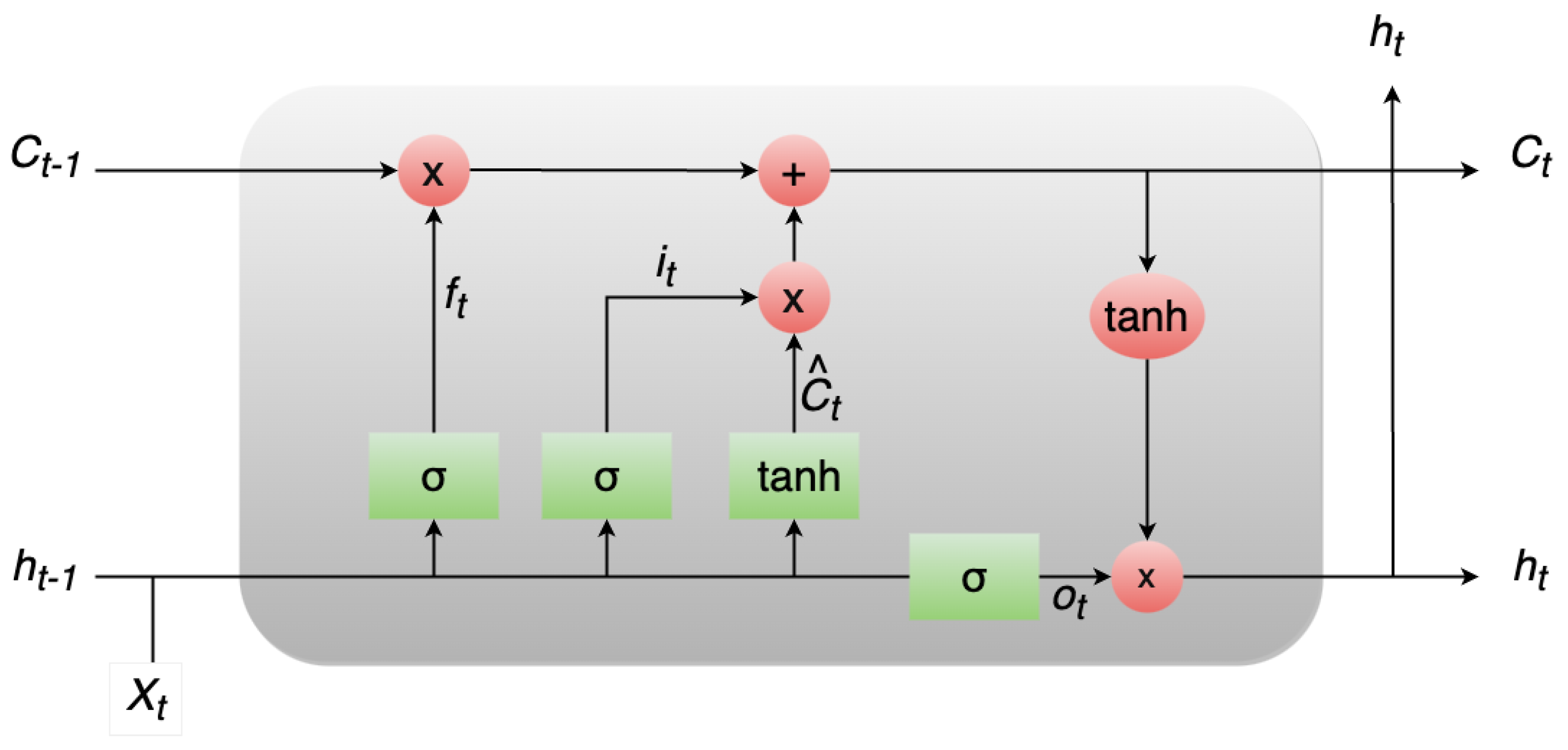
In 1997, Hochreiter and Schmidhuber introduced LSTM networks [31] as a specialized variant of RNNs tailored to effectively manage and learn from long-term dependencies in data. Their pervasive adoption and demonstrated success across a range of problem domains have propelled LSTMs into heightened prominence. Unlike traditional RNNs, LSTMs are explicitly engineered to tackle the challenge of prolonged dependencies, constituting an innate feature of their functioning. LSTMs are constructed from a sequence of recurrent modules, a common trait shared with all RNNs. Yet, it is the configuration of these repeating modules that sets LSTMs apart. In contrast to a solitary layer, LSTMs encompass four interconnected layers. The pivotal distinction within LSTMs arises from the incorporation of a cell state—a horizontal conduit running through the modules that orchestrate seamless information propagation. The transmission of data within the cell state is governed by gates, which comprise a neural network layer based on the sigmoid function connected with a pointwise multiplication operation. The sigmoid layer generates values in the range of 0 to 1, dictating the extent of the passage of information. The fundamental architecture of the LSTM model is visually depicted in Figure 1.

Figure 1.
The LSTM model architecture.
To regulate the cell state, LSTM networks employ three distinct gates: the forget gate, the input gate, and the output gate. The purpose of the forget gate is to employ a sigmoid layer to determine which elements of information should be omitted from the current cell state. The input gate is composed of two key elements: a sigmoid layer, responsible for regulating the updates to be applied, and a tangent hyperbolic (tanh) layer, which generates new potential values. These new pieces of information are then combined with the existing cell state to generate an updated state. The output gate, on the other hand, employs a sigmoid layer to discern the relevant segments of the cell state that are pertinent to the final output. This processed cell state is subsequently passed through a tanh activation function and multiplied by the output obtained from the sigmoid gate. This combined process ultimately results in the final output. Here, represents the input at a given time step, signifies the output, represents the cell state, corresponds to the forget gate, denotes the input gate, represents the output gate, and signifies the internal cell state.
2.2. BiLSTM
The BiLSTM network [32] constitutes a sophisticated variant of the LSTM architecture. LSTM, in itself, is a specialized form of Recurrent Neural Network (RNN) that has been proven effective in handling sequential data, such as text, speech, and time-series data. However, standard LSTM models have limitations when it comes to capturing bidirectional dependencies within the data, which is where BiLSTM steps in to overcome this constraint. At its core, the BiLSTM network introduces bidirectionality by processing input sequences both forward and backward through two separate LSTM layers. By doing so, the model can exploit context from past and future information simultaneously, leading to a more comprehensive understanding of the data. This distinctive competence renders it especially apt for endeavors necessitating a profound examination of sequential patterns, such as sentiment analysis, named entity recognition, machine translation, and related tasks. The key advantages of bidirectional LSTMs are:
- Enhanced Contextual Understanding: By considering both past and future information, bidirectional LSTMs better understand the context surrounding each time step in a sequence. This is particularly useful for tasks where the meaning of a word or a data point is influenced by its surrounding elements.
- Long-Range Dependencies: Bidirectional LSTMs can capture long-range dependencies more effectively than unidirectional LSTMs. Information from the future can provide valuable insights into the context of earlier parts of the sequence.
- Improved Performance: In tasks like sequence labeling, sentiment analysis, and machine translation, bidirectional LSTMs often outperform unidirectional LSTMs because they can better capture nuanced relationships between elements in a sequence.
However, bidirectional LSTMs also come with certain considerations:
- Computational Complexity: Since bidirectional LSTMs process data in two directions, they are computationally more intensive than their unidirectional counterparts. This can result in extended training durations and elevated memory demands.
- Real-Time Applications: In real-time applications where future information is not available, bidirectional LSTMs might not be suitable, as they inherently use both past and future context.
- Causal Relationships: Bidirectional LSTMs may introduce possible causality violations when used in scenarios where future information is not realistically available at present.
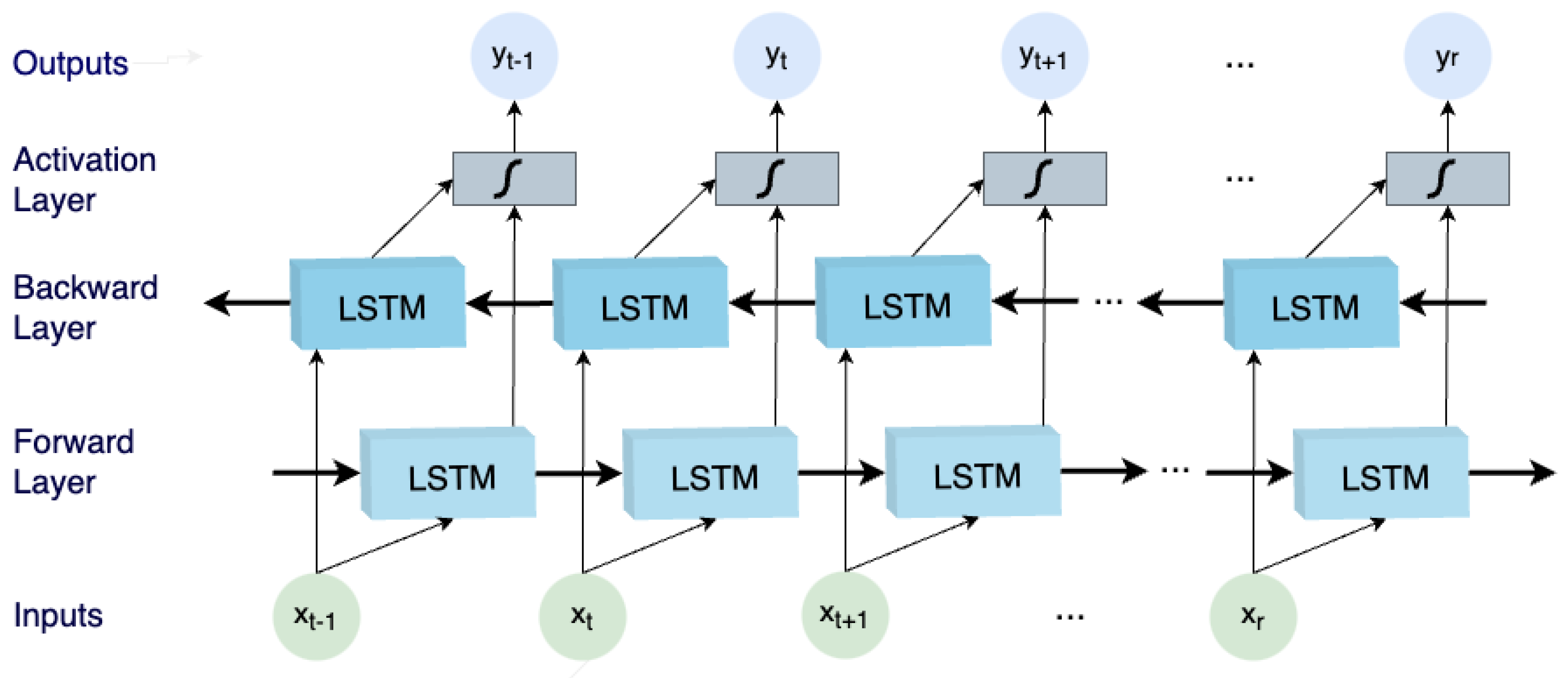
Analyzing each component of a BiLSTM network provides valuable insights into its inner workings and how it overcomes the limitations of traditional LSTMs. A BiLSTM network comprises four main components, i.e., input layer, LSTM layers (both forward and backward), merging layer, and output layer. Next, a detailed analysis of the components is provided:
- Input Layer: The input layer is the first step in the BiLSTM network and serves as the entry point for sequential data. It accepts the input sequence, which could be a sequence of words in natural language processing tasks or time-series data in other applications. The data is typically encoded using word embeddings or other numerical representations to enable the network to process it effectively. The input layer bears the responsibility of transforming the unprocessed input into a structure comprehensible by subsequent layers.
- LSTM Layers (Forward and Backward): The fundamental element of the BiLSTM network is composed of two LSTM layers: one dedicated to sequentially processing the input sequence in a forward manner, while the other focuses on processing it in a reverse direction. These LSTM layers play a pivotal role in capturing temporal correlations and extensive contextual information embedded within the data. In the forward LSTM layer, the input sequence is systematically processed from the sequence’s initiation to its conclusion, whereas in the backward LSTM layer, the sequence is processed in a reverse manner. By encompassing dual-directional data processing, the BiLSTM effectively captures insights from both historical and prospective facets of the input, enabling adept modeling of bidirectional relationships. Each LSTM cell situated within these layers incorporates a set of gating mechanisms—namely, input, output, and forget gates—that meticulously govern the course of information flow within the cell. This orchestration ensures the network’s retention of crucial information over extended temporal spans, thereby mitigating the issue of vanishing gradients and substantially enhancing gradient propagation during the training phase.
- Merging/Activation Layer: Following the sequential processing by the forward and backward LSTM layers, the fusion layer takes center stage. The principal aim of this layer is to seamlessly amalgamate the insights garnered from both directions. This amalgamation is typically accomplished by concatenating the hidden states of the forward and backward LSTMs at each discrete time step. This concatenated representation thus encapsulates knowledge encompassing both anterior and forthcoming contexts for every constituent within the input sequence. This amalgamated representation serves as the fundamental bedrock upon which the ensuing layers base their informed decisions, enriched by bidirectional context.
- Output Layer: Serving as the ultimate stage within the BiLSTM network, the outcome generation layer undertakes the task of processing the concatenated representation obtained from the fusion layer to yield the intended output. The design of the outcome generation layer depends on the specific objective customized for the BiLSTM. For example, in sentiment analysis, this layer might comprise a solitary node featuring a sigmoid activation function to predict sentiment polarity (positive or negative). In alternative applications like machine translation, the outcome layer could encompass a softmax activation function aimed at predicting the probability distribution of target words within the translation sequence. The outcome layer assumes the responsibility of mapping the bidirectional context, assimilated by the BiLSTM, into the conclusive predictions or representations that align with the precise objectives of the designated task.
The basic architecture of the BiLSTM model including the above-mentioned layers is visually depicted in Figure 2.
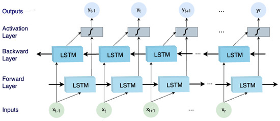
Figure 2.
The BiLSTM basic architecture.
In summary, a bidirectional LSTM stands as an extension of the conventional LSTM architecture, adeptly harnessing information originating from both past and future time steps. This augmentation substantially enhances the comprehension of sequential data, capturing intricate patterns and interrelationships. As such, bidirectional LSTMs emerge as a potent instrument for diverse sequence-oriented tasks within the realms of machine learning and deep learning.
3. Materials and Methods
3.1. Forming the Training and Testing Set
The dataset encompasses the hourly energy consumption data for Greece over 746 days, spanning from 31 November 2020 to 16 December 2022, as reported by Independent Power Transmission Operator (IPTO) S.A. [33], which assumes the role of Owner and Operator of the Hellenic Electricity Transmission System (HETS). The core objective of IPTO encompasses the oversight, regulation, upkeep, and advancement of the HETS. In constructed dataset, every individual data point present represents the energy consumption for a particular hour, denominated in megawatt-hours (MWh). In essence, for each day, a sequence of 24 energy indices is provided, each representing the energy consumption for a respective hour.
3.2. Software Tools and Frameworks
In the training and testing process of the models, a suite of essential Python libraries was utilized. These included Pandas and NumPy, which were employed for proficient data preprocessing and manipulation. The Keras library, particularly its Sequential model, was employed to provide a user-friendly and robust framework for the construction and training of neural networks, simplifying the implementation of deep learning architectures. Additionally, Scikit-learn (sklearn) emerged as a valuable asset for the model evaluation, the fine-tuning of the models, and the optimization of their performance. The integration of these libraries in the research process ensured an efficient and effective workflow, resulting in high-quality results and conclusions presented in this paper.
3.3. Proposed Methodology
The proposed model for forecasting electricity demand leverages the power of BiLSTM networks to effectively capture temporal dependencies and contextual information in energy consumption data (see Algorithm 1). The proposed research extends from earlier study [34] concentrated on employing artificial neural networks to attain precise predictions of electrical load. The model architecture comprises multiple layers that enable it to learn and predict energy load patterns more accurately. At the core of the architecture are two Bidirectional LSTM layers, each working in tandem to extract valuable insights from the sequential input data. The first Bidirectional LSTM layer processes the input data, which is a time series of energy consumption values. This layer’s bidirectional nature allows it to simultaneously analyze the temporal sequence in both forward and backward directions. This is particularly advantageous in energy load prediction, as it enables the model to consider past consumption patterns as well as anticipate future trends. Following the first BiLSTM layer is another BiLSTM layer that further refines the representations learned in the previous layer. This layer efficiently encodes the enriched context from the first layer and generates more abstract and high-level features. The bidirectional processing ensures that the model is not limited to capturing only past context but also takes advantage of information from the future, enhancing its understanding of the intricate relationships between energy consumption values. The final layer of the architecture is a dense layer, responsible for producing the prediction output. This dense layer takes the representations learned by the preceding BiLSTM layers and transforms them into a single output value. This value corresponds to the predicted energy load for the next time step.
The transformation necessitates learned weights and biases, which undergo refinement during the training phase to minimize prediction errors. The deep learning model proposed for energy load prediction underwent an extensive training regimen spanning 40 epochs, employing the Adam optimizer. The Adam optimizer, known for its adaptive learning rate and momentum, facilitated the optimization of the model’s weights and biases throughout the training process. In terms of architecture parameters, the model is equipped with a total of 81,301 trainable parameters. These parameters are adjusted during training to optimize the model’s performance in making accurate energy-load predictions.
| Algorithm 1 Energy Consumption Prediction Algorithm |
Input: Historical energy consumption data for Greece Output: Predicted energy consumption
|
4. Experimental Results
Table 1 provides a comprehensive analysis of RMSE and MAE (see Equations (1) and Equation (2), respectively) errors for four distinct neural network architectures—BiLSTM, RNN, LSTM, and GRU—across varying time steps (12, 24, 48, and 72 h). MAE is a common metric used to measure the average absolute difference between the actual values () and the predicted values () in a dataset. It provides a simple and straightforward way to assess the accuracy of a predictive model. A smaller MAE indicates a better model fit, and the values are not squared, so outliers have a linear effect on the metric. RMSE is also common metric for evaluating the accuracy of a predictive model. It measures the square root of the average of the squared differences between actual values () and predicted values (). RMSE places more weight on large errors due to the squaring of differences, making it sensitive to outliers. The performance of each architecture is evaluated on both training and testing sets, shedding light on their predictive capabilities for energy load forecasting.

Table 1.
RMSE and MAE comparison for the four proposed neural networks across different time steps in training and testing sets.
The BiLSTM architecture demonstrates superior predictive capabilities for energy load forecasting across different time steps, as highlighted in the provided table. Comparing its performance to the other architectures, the BiLSTM consistently yields the lowest RMSE and MAE values on both the training and testing sets.
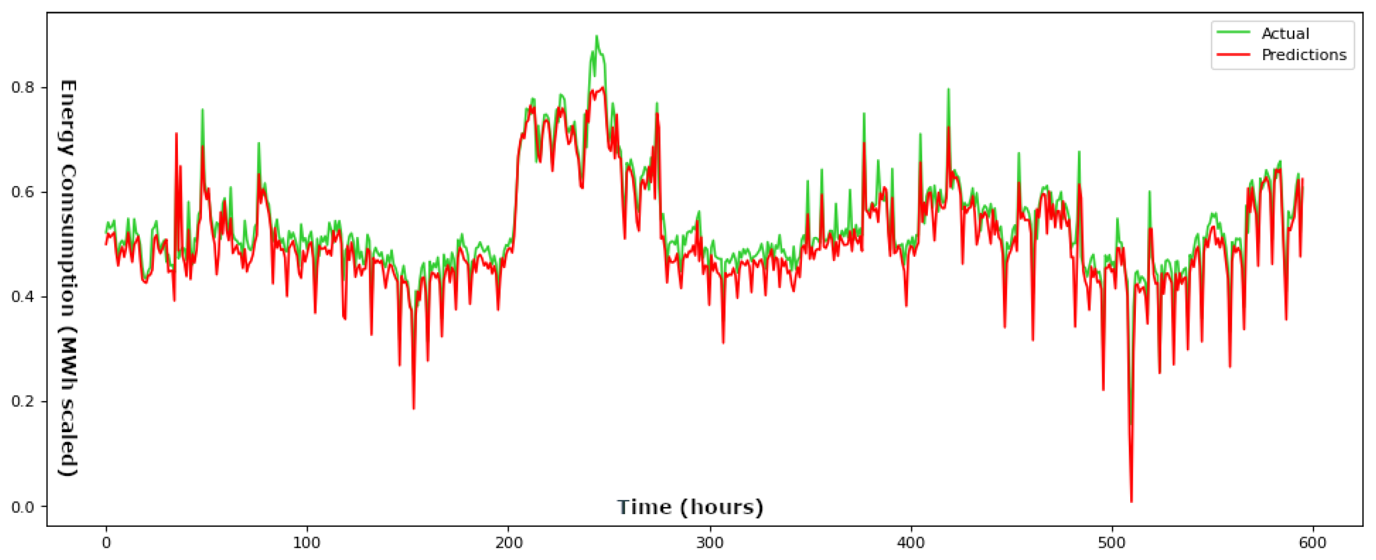
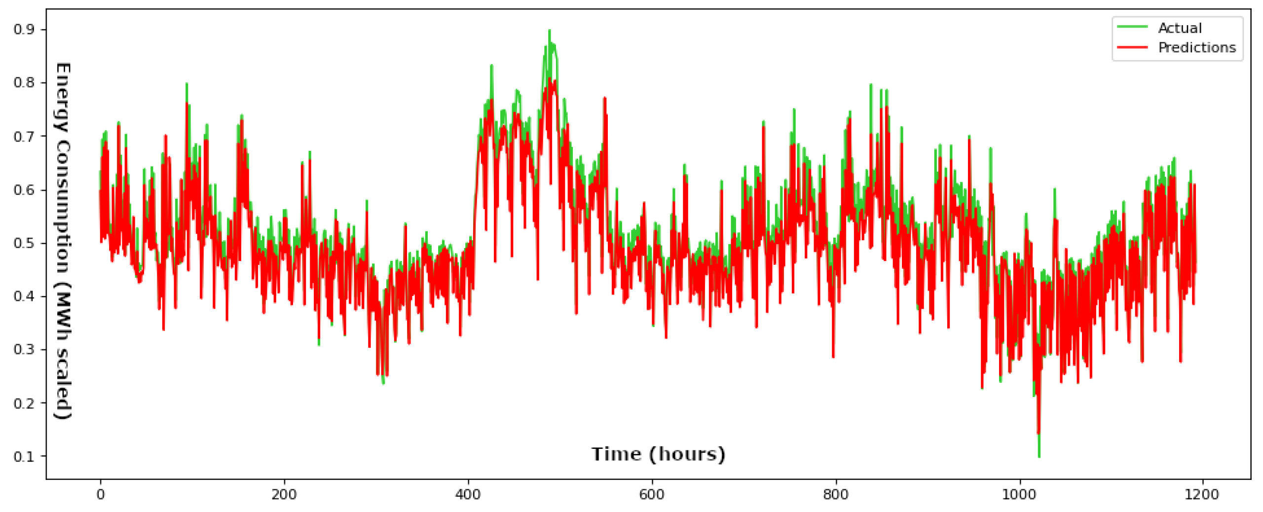
In Figure 3 and Figure 4, the comparison between the real ground truth values and the corresponding predicted values is demonstrated for a time step parameter set at 24 h, for both the training and testing phases. Our conducted analysis reveals that employing a time step of 24 h yields the most optimal outcomes within the test dataset. This specific time step yields minimal RMSE and MAE values, indicating a robust 24-h periodicity.
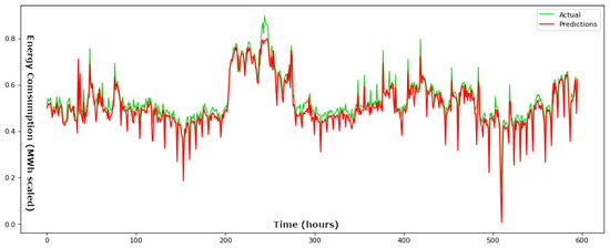
Figure 3.
Actual values compared to the predicted values throughout the training phase for a time step parameter set at 24 h for the suggested BiLSTM framework.
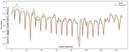
Figure 4.
Actual values compared to the predicted values throughout the testing phase for a time step parameter set at 24 h for the suggested BiLSTM framework.
Next, in Figure 5, Figure 6, Figure 7, Figure 8, Figure 9 and Figure 10, the comparison between the ground truth values and their corresponding predictions is illustrated for time step parameters 12, 48, and 72 h, corresponding to the training and testing phases, respectively.
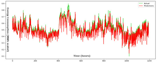
Figure 5.
Actual values compared to the predicted values throughout the training phase for a time step parameter set at 12 h for the suggested BiLSTM framework.
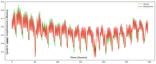
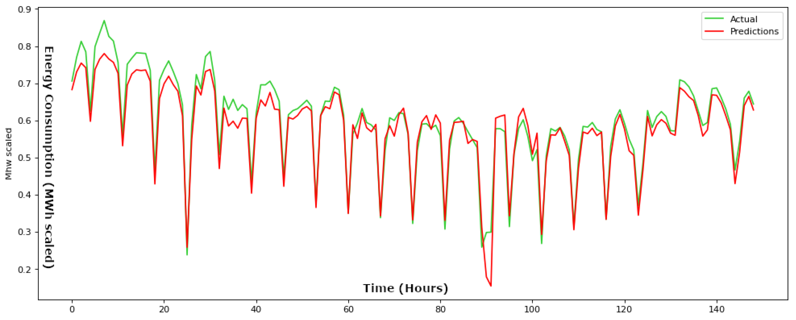
Figure 6.
Actual values compared to the predicted values throughout the testing phase for a time step parameter set at 12 h for the suggested BiLSTM framework.
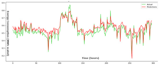
Figure 7.
Actual values compared to the predicted values throughout the training phase for a time step parameter set at 48 h for the suggested BiLSTM framework.
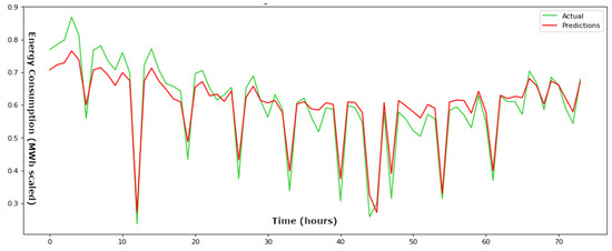
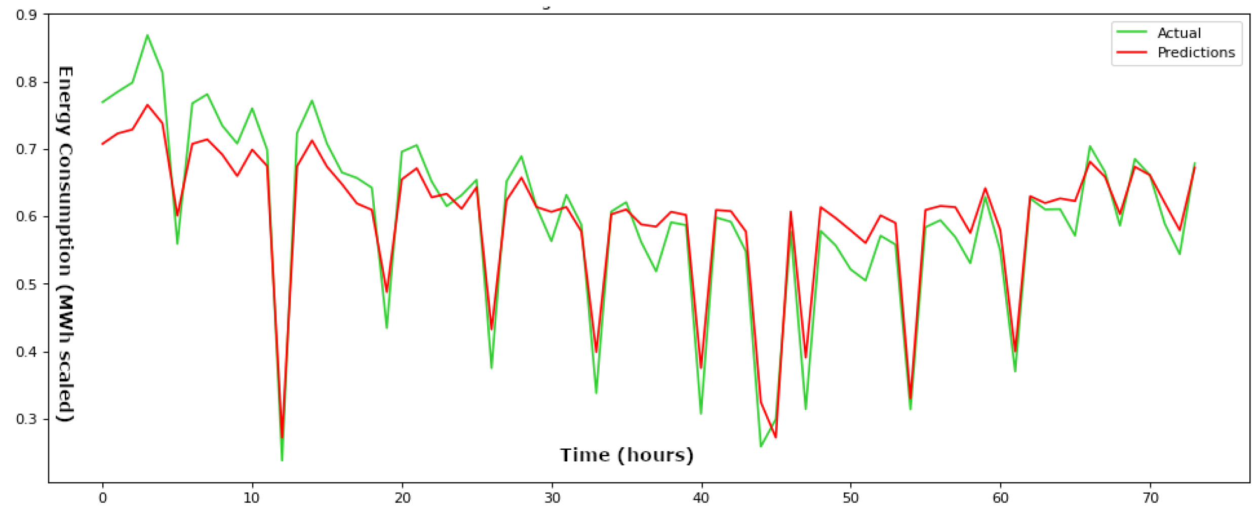
Figure 8.
Actual values compared to the predicted values throughout the testing phase for a time step parameter set at 48 h for the suggested BiLSTM framework.
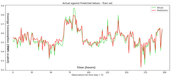
Figure 9.
Actual values compared to the predicted values throughout the training phase for a time step parameter set at 72 h for the suggested BiLSTM framework.
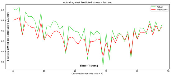
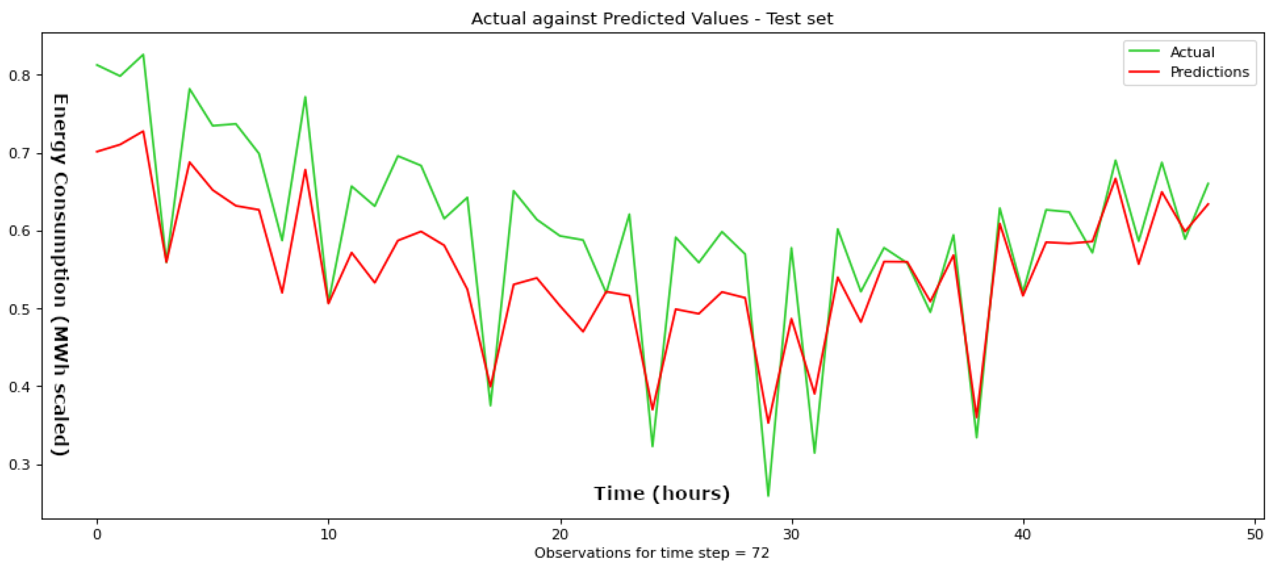
Figure 10.
Actual values compared to the predicted values throughout the testing phase for a time step parameter set at 72 h for the suggested BiLSTM framework.
In the training set, the BiLSTM achieves remarkable results, with an RMSE of 0.019 for the 12-h time step, outperforming the RNN (0.032), LSTM (0.024), and GRU (0.026) by approximately 41%, 21%, and 27%, respectively. The BiLSTM also showcases its superiority at longer time steps, with RMSE values of 0.025, 0.027, and 0.026 for time steps of 24, 48, and 72 h, respectively. For the 24-h time-step, it outperforms the RNN by approximately 35%, the LSTM by 17%, and the GRU by 22%. The same percentages for the 48-h time-step are 48% (RNN), 10% (LSTM), and 7% (GRU).
Finally, in the case of the 72-h time step, the BiLSTM outperforms the RNN by approximately 19%, the LSTM by 52%, and the GRU by 17%. In terms of MAE, the BiLSTM also presents impressive performance. At the 12-h time step, its MAE of 0.113 significantly outperforms the RNN (0.161), the LSTM (0.129), and GRU (0.137) by approximately 30%, 12%, and 17%, respectively. This advantage extends to longer time steps, where the BiLSTM demonstrates MAE values of 0.133, 0.139, and 0.135 for time steps of 24, 48, and 72 h, respectively.
Against the RNN, the LSTM, and the GRU, the BiLSTM maintains leads ranging from around 17% TO 34% for the RNN, 8% to 38% for the LSTM, and 4% to 7% for the GRU.
Turning to the testing set, the BiLSTM proves to be equally accurate or even more accurate than the other networks. At the 12-h time step, its RMSE of 0.053 is comparable to that of the RNN (0.048), LSTM (0.050), and GRU (0.057). Moving to the 24-h time step, the BiLSTM’s RMSE of 0.022 is notably lower than that of the RNN (0.033), LSTM (0.055), and GRU (0.033). This indicates an impressive error reduction of approximately 60% against the LSTM and 33% against the GRU and the RNN. Only at the 48-h and 72-h time steps does the GRU consistently outperform both the BiLSTM and LSTM in terms of RMSE values. Regarding MAE, the superiority of BiLSTM remains pronounced, particularly at the 24-h time step, which yields the best testing result among all examined variations. For the 12-h time step, its MAE of 0.167 is comparable to that of the RNN (0.165), LSTM (0.162), and GRU (0.188). At the 24-h time step, as mentioned earlier, the BiLSTM’s MAE of 0.122 demonstrates remarkable accuracy, outperforming the RNN (0.163), LSTM (0.228), and GRU (0.165) by approximately 25%, 46%, and 26%, respectively. As the time step extends to 48 and 72 h, the BiLSTM exhibits slightly lower values compared to the RNN and GRU. In both cases, the MAE is comparable for the BiLSTM and LSTM. Specifically, the BiLSTM performs better at the 72-h time step, while the LSTM shows a slight advantage at the 24-h time step.
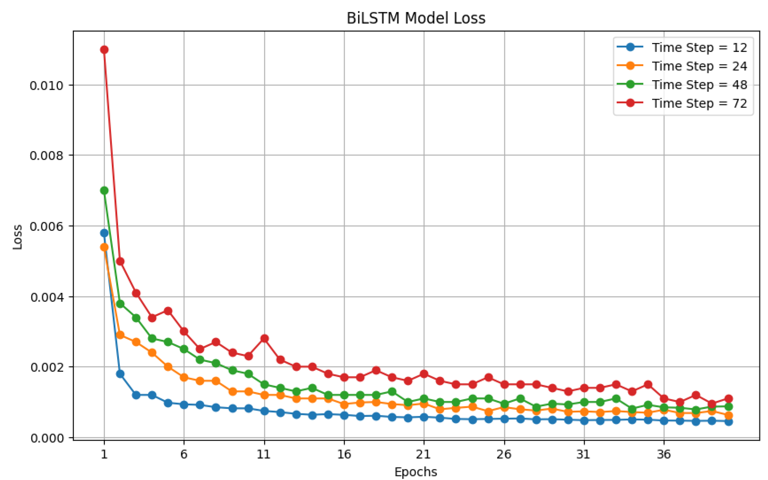
Finally, Figure 11 illustrates the evolution of the loss function throughout the training epochs for the BiLSTM network. The prevailing trend in most cases demonstrates a consistent decrease in the loss function, followed by a period of stability that indicates the proposed networks are converging towards a dependable solution. This suggests the model’s adeptness in capturing underlying patterns and its effective performance on the training dataset. The convergence observed in the loss function curve serves as an indicator of an appropriately chosen learning rate, evident in its smooth and consistent convergence trajectory.
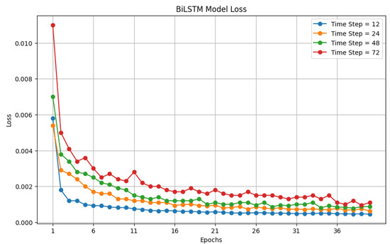
Figure 11.
The progression of the loss function during the training epochs for the biLSTM network for time steps 12, 24, 48, and 72 h.
5. Conclusions
In conclusion, this paper presents an extended study on electrical load prediction by introducing an enhanced framework based on a bidirectional Long Short-Term Memory (BiLSTM) neural network. Unlike traditional feed-forward networks, the bidirectional LSTM model captures sequential dependencies in energy consumption data, allowing it to effectively store and utilize information from both past and future time steps. The comprehensive analysis of various neural network architectures reveals that the proposed BiLSTM architecture consistently outperforms other models, including RNN, LSTM, and GRU, across multiple time steps, and specifically presents the best results of all networks and time steps for the 24-h time-step variation. It achieves remarkable accuracy in terms of RMSE and MAE errors on both training and testing sets. Specifically, the BiLSTM’s MAE of 0.122 demonstrates remarkable accuracy, outperforming the RNN (0.163), LSTM (0.228), and GRU (0.165) by approximately 25%, 46%, and 26%, in the best variation of all networks, at 24-h time step, while the BiLSTM’s RMSE of 0.022 is notably lower than that of the RNN (0.033), LSTM (0.055), and GRU (0.033), respectively. The superiority of BiLSTM is evident across different time steps, demonstrating substantial reductions in prediction errors compared to other architectures. This study underscores the significance of incorporating advanced neural network architectures, particularly bidirectional memory-based models like BiLSTM, in enhancing the accuracy of energy load forecasting. The findings contribute to more precise energy planning, market management, and decision-making processes within power systems. Our future goal is to develop dedicated hardware modules that will produce short-term real-time predictions using the methodologies and techniques proposed in [35,36,37].
Author Contributions
Conceptualization, C.P., V.M. and E.M.; methodology, G.F.; software, E.M.; validation, C.P. and V.V.; formal analysis, G.F., V.V. and V.M.; investigation, G.F. and C.P.; resources, G.F.; writing—original draft preparation, C.P., E.M. and G.F.; writing—review and editing, E.M.; visualization, V.V.; supervision, C.P. and V.M.; project administration, G.F. and V.M. All authors have read and agreed to the published version of the manuscript.
Funding
This research received no external funding.
Data Availability Statement
Publicly available datasets were analyzed in this study. This data can be found here: https://www.data.gov.gr/datasets/admie_realtimescadasystemload/.
Conflicts of Interest
The authors declare no conflict of interest.
Abbreviations
The following abbreviations are used in this manuscript:
| AGC | Automatic Generation Control |
| ANN | Artificial Neural Network |
| BiLSTM | Bidirectional Long Short-Term Memory |
| CNN | Convolutional Neural Network |
| DSO | Distribution System Operators |
| ELD | Economic Load Dispatch |
| GRU | Gated Recurrent Unit |
| HETS | Hellenic Electricity Transmission System |
| IPTO | Independent Power Transmission Operator |
| LD | Linear dichroism |
| LSTM | Long Short-Term Memory |
| LTF | Long-term forecasting |
| MAE | Mean Absolute Error |
| MTF | Medium-term forecasting |
| RMSE | Root Mean Square Error |
| RNN | Recurrent Neural Network |
| STF | Short-term forecasting |
| TSO | Transmission System Operator |
References
- Kang, C.; Xia, Q.; Zhang, B. Review of power system load forecasting and its development. Autom. Electr. Power Syst. 2004, 28, 1–11. [Google Scholar]
- Zhang, K.; Feng, X.; Tian, X.; Hu, Z.; Guo, N. Partial Least Squares regression load forecasting model based on the combination of grey Verhulst and equal-dimension and new-information model. In Proceedings of the 7th International Forum on Electrical Engineering And Automation (IFEEA), Hefei, China, 25–27 September 2020; pp. 915–919. [Google Scholar] [CrossRef]
- Liu, Z.; Sun, X.; Wang, S.; Pan, M.; Zhang, Y.; Ji, Z. Midterm Power Load Forecasting Model Based on Kernel Principal Component Analysis. Big Data 2019, 7, 130–138. [Google Scholar] [CrossRef]
- Al-Hamadi, H.M.; Soliman, S.A. Long-term/mid-term electric load forecasting based on short-term correlation and annual growth. Electr. Power Syst. Res. 2005, 74, 353–361. [Google Scholar] [CrossRef]
- Baek, S. Mid-term Load Pattern Forecasting with Recurrent Artificial Neural Network. IEEE Access 2019, 7, 172830–172838. [Google Scholar] [CrossRef]
- Nalcaci, G.; Özmen, A.; Weber, G.W. Long-term load forecasting: Models based on MARS, ANN and LR methods. Cent. Eur. J. Oper. Res. 2019, 27, 1033–1049. [Google Scholar] [CrossRef]
- Adhiswara, R.; Abdullah, A.G.; Mulyadi, Y. Long-term electrical consumption forecasting using Artificial Neural Network (ANN). J. Phys. Conf. Ser. 2019, 1402, 033081. [Google Scholar] [CrossRef]
- Abu-Shikhah, N.; Aloquili, F.; Linear, O.; Regression, N. Medium-Term Electric Load Forecasting Using Multivariable Linear and Non-Linear Regression. Smart Grid Renew. Energy 2011, 2, 126–135. [Google Scholar] [CrossRef]
- Krstonijević, S. Adaptive Load Forecasting Methodology Based on Generalized Additive Model with Automatic Variable Selection. Sensors 2022, 22, 7247. [Google Scholar] [CrossRef] [PubMed]
- Ono, M.; Topcu, U.; Yo, M.; Adachi, S. Risk-limiting power grid control with an ARMA-based prediction model. In Proceedings of the 2013 IEEE 52nd Annual Conference on Decision and Control, CDC 2013, Firenze, Italy, 10–13 December 2013; pp. 4949–4956. [Google Scholar]
- Shi, T.; Lu, F.; Lu, J.; Pan, J.; Zhou, Y.; Wu, C.; Zheng, J. Phase Space Reconstruction Algorithm and Deep Learning-Based Very Short-Term Bus Load Forecasting. Energies 2019, 12, 4349. [Google Scholar] [CrossRef]
- Román-Portabales, A.; López-Nores, M.; Pazos-Arias, J.J. Systematic Review of Electricity Demand Forecast Using ANN-Based Machine Learning Algorithms. Sensors 2021, 21, 4544. [Google Scholar] [CrossRef]
- Ekonomou, L.; Christodoulou, C.A.; Mladenov, V. A short-term load forecasting method using artificial neural networks and wavelet analysis. Int. J. Power Syst. 2016, 1, 64–68. [Google Scholar]
- Karampelas, P.; Pavlatos, C.; Mladenov, V.; Ekonomou, L. Design of artificial neural network models for the prediction of the Hellenic energy consumption, In Proceedings of the 10th Symposium on Neural Network Applications in Electrical Engineering, Belgrade, Serbia, 23–25 September 2010.
- Hwan, K.J.; Kim, G.W. A short-term load forecasting expert system. In Proceedings of the 5th Korea-Russia International Symposium On Science And Technology, Tomsk, Russia, 26 June–3 July 2001; Volume 1, pp. 112–116. [Google Scholar]
- Ali, M.; Adnan, M.; Tariq, M.; Poor, H.V. Load Forecasting Through Estimated Parametrized Based Fuzzy Inference System in Smart Grids. IEEE Trans. Fuzzy Syst. 2021, 29, 156–165. [Google Scholar] [CrossRef]
- Bhotto, M.Z.A.; Jones, R.; Makonin, S.; Bajić, I.V. Short-Term Demand Prediction Using an Ensemble of Linearly-Constrained Estimators. IEEE Trans. Power Syst. 2021, 36, 3163–3175. [Google Scholar] [CrossRef]
- Jiang, H.; Zhang, Y.; Muljadi, E.; Zhang, J.J.; Gao, D.W. A Short-Term and High-Resolution Distribution System Load Forecasting Approach Using Support Vector Regression with Hybrid Parameters Optimization. IEEE Trans. Smart Grid 2018, 9, 3341–3350. [Google Scholar] [CrossRef]
- Li, G.; Li, Y.; Roozitalab, F. Midterm Load Forecasting: A Multistep Approach Based on Phase Space Reconstruction and Sup-port Vector Machine. IEEE Syst. J. 2020, 14, 4967–4977. [Google Scholar] [CrossRef]
- Zafeiropoulou, M.; Mentis, I.; Sijakovic, N.; Terzic, A.; Fotis, G.; Maris, T.I.; Vita, V.; Zoulias, E.; Ristic, V.; Ekonomou, L. Forecasting Transmission and Distribution System Flexibility Needs for Severe Weather Condition Resilience and Outage Management. Appl. Sci. 2022, 12, 7334. [Google Scholar] [CrossRef]
- Fotis, G.; Vita, V.; Maris, I.T. Risks in the European Transmission System and a Novel Restoration Strategy for a Power System after a Major Blackout. Appl. Sci. 2023, 13, 83. [Google Scholar] [CrossRef]
- Zheng, C.; Eskandari, M.; Li, M.; Sun, Z. GA-Reinforced Deep Neural Network for Net Electric Load Forecasting in Microgrids with Renewable Energy Resources for Scheduling Battery Energy Storage Systems. Algorithms 2022, 15, 338. [Google Scholar] [CrossRef]
- Sambhi, S.; Bhadoria, H.; Kumar, V.; Chaurasia, P.; Chaurasia, G.S.; Fotis, G.; Vita, G.; Ekonomou, V.; Pavlatos, C. Economic Feasibility of a Renewable Integrated Hybrid Power Generation System for a Rural Village of Ladakh. Energies 2022, 15, 9126. [Google Scholar] [CrossRef]
- Khuntia, S.; Rueda, J.; Meijden, M. Forecasting the load of electrical power systems in mid- and long-term horizons: A review. IET Gener. Transm. Distrib. 2016, 10, 3971–3977. [Google Scholar] [CrossRef]
- THong, A.; Pinson, P.; Fan, S.; Zareipour, H.; Troccoli, A. Electricity Load Forecasting: A Survey. IEEE Trans. Smart Grid 2016, 7, 1040–1071. [Google Scholar]
- IRENA. Innovation Landscape Brief: Market Integration of Distributed Energy Resources; International Renewable Energy Agency: Abu Dhabi, United Arab Emirates, 2019. [Google Scholar]
- Commission, M.; Company, D. Integrating Renewables into Lower Michigan Electric Grid. Available online: https://www.brattle.com/wp-content/uploads/2021/05/15955_integrating_renewables_into_lower_michigans_electricity_grid.pdf (accessed on 14 November 2023).
- Wang, F.C.; Hsiao, Y.S.; Yang, Y.Z. The Optimization Of Hybrid Power Systems With Renewable Energy And Hydrogen Gen-eration. Energies 2018, 11, 1948. [Google Scholar] [CrossRef]
- Wang, F.; Lin, K.-M. Impacts Of Load Profiles On The Optimization Of Power Management Of A Green Building Employing Fuel Cells. Energies 2019, 12, 57. [Google Scholar] [CrossRef]
- Sun, W.; Zhang, C. A Hybrid BA-ELM Model Based on Factor Analysis and Similar-Day Approach for Short-Term Load Forecasting. Energies 2018, 11, 1282. [Google Scholar] [CrossRef]
- Hochreiter, S.; Schmidhuber, J. Long short-term memory. Neural Comput. 1997, 9, 1735–1780. [Google Scholar] [CrossRef] [PubMed]
- Graves, A.; Schmidhuber, J. Framewise phoneme classification with bidirectional LSTM and other neural network architectures, JCNN’05. In Proceedings of the 2005 IEEE International Joint Conference on Neural Networks, Montreal, QC, Canada, 31 July–4 August 2005; pp. 2047–2052. [Google Scholar]
- Available online: https://www.data.gov.gr/datasets/admie_realtimescadasystemload/ (accessed on 26 August 2023).
- Pavlatos, C.; Makris, E.; Fotis, G.; Vita, V.; Mladenov, V. Utilization of Artificial Neural Networks for Precise Electrical Load Prediction. Technologies 2023, 11, 70. [Google Scholar] [CrossRef]
- Panagopoulos, I.; Pavlatos, C.; Papakonstantinou, G.K. An Embedded System for Artificial Intelligence Applications. World Acad. Sci. Eng. Technol. Int. J. Comput. Electr. Autom. Control Inf. Eng. 2007, 1, 1155–1169. [Google Scholar]
- Pavlatos, C.; Vita, V.; Ekonomou, L. Syntactic pattern recognition of power system signals. In Proceedings of the 19th WSEAS International Conference on Systems, Zakynthos Island, Greece, 16–20 July 2015. [Google Scholar]
- Pavlatos, C.; Dimopoulos, A.; Papakonstantinou, G. An intelligent embedded system for control applications. In MCCS’05, Workshop on Modeling and Control of Complex Systems, Cyprus; 2005. [Google Scholar]


Disclaimer/Publisher’s Note: The statements, opinions and data contained in all publications are solely those of the individual author(s) and contributor(s) and not of MDPI and/or the editor(s). MDPI and/or the editor(s) disclaim responsibility for any injury to people or property resulting from any ideas, methods, instructions or products referred to in the content. |
© 2023 by the authors. Licensee MDPI, Basel, Switzerland. This article is an open access article distributed under the terms and conditions of the Creative Commons Attribution (CC BY) license (https://creativecommons.org/licenses/by/4.0/).