Abstract
Pure electric public transport management optimization can promote the electrification evolution from conventional diesel emission to low/zero carbon transport revolution. However, emerging electric vehicle scheduling (EVS) takes into account battery capacity, battery-allowed mileage, and charging duration, which are a few concerns present at the conventional motor bus planning level. Concentrating on this new challenge, this paper builds a multi-type electric vehicle scheduling model, featuring rigorous load capacity, battery-allowed mileage, and recharging duration constraints. The binary decision variables involving the connection between departure and arrival times, as well as the recharging necessity, are judged simultaneously. The objective is to minimize the fleet size, idle mileage, and charging cost. A preprocessing-based genetic algorithm is used to handle this mixed-integer nonlinear programing model. Numerical examples are tested to validate the effectiveness of the proposed models and the solution algorithm. Compared with a single large-type vehicle scheme, the total cost of multi-type vehicle scheduling in one-trip, two-trip, and three-trip frequency scenarios are reduced by 20.8%, 6.3%, and 9.1%, respectively.
1. Introduction
With the development of urbanization, the continuous surge in the number of diesel buses leads to a significant amount of energy consumption and pollution emissions. Conventional diesel buses not only pollute the air and aggravate the greenhouse effect, but also restrict the sustainable development of the public transport (PT) system. Motivated by national policies in China, different types of pure electric public transport vehicles (EPTVs) are widely used in large- and medium-sized cities to solve these diesel-caused, environment-related problems. In recent years, pure electric vehicles have gradually become a hot spot in the field of transportation. However, the restricted driving range and the necessary recharging time of EPTVs require prudent energy optimization management for vehicle scheduling. The term ‘energy optimization’ refers to recharging queuing, recharger utilization, recharging duration, and battery health life. In order to handle a series of recharging scheduling issues, we propose a multi-type electric vehicle scheduling (EVS) model to facilitate an optimal fleet size deployment and save the net operation interest.
Owing to the environmental appeal of pure electric buses, various vehicle types are provided as on-demand options in the daily PT operation level. On the contrary, in terms of single type vehicle scheduling, it is hard to cope with the time-depended passenger distribution derived from the fluctuation between peak and off-peak hours. Thus, multi-type electric-vehicle schedule optimization is a novel work in this paper. The aim is not only to reduce the fleet size purchase cost, but also provide a reasonable load capacity. In particular, a bigger load capacity benefits for the accommodation of crowded users and vice versa. Furthermore, pure electric PT vehicle type attributes with different properties. On one hand, the larger vehicle type refers to a big battery with a longer recharging time window, which leads to a higher purchase price. On the other hand, the small vehicle type has the opposite attributes. Our motivation is to strictly consider these nature-based constraints, namely, different battery-allowed mileage, recharging times, and energy consumption, in order to propose a precise multi-type EVS model.
It is known that the classical vehicle scheduling (VS) model is used to facilitate the optimized order of trips, service frequencies, departure times, and fleet size. Given an environment-friendly opportunity to promote electrical PT, we are rising to the challenge of dealing with recharging scheduling management. Another major difficulty of optimizing the electrical PT vehicle schedule is derived from the multi-type EPTV selections. In this study, we build a multi-objective integer nonlinear programing (MINLP) model with the following three objectives: to minimize fleet size, idle mileage, and recharging costs. With a single one-type vehicle schedule, it is hard to attain the trade-off between supply resources and user demand. This is the motivation for why this study concentrates on multi-type EVS yielding with different battery-allowed mileage, recharging time, and energy consumption.
In order to avoid/alleviate both PT resource waste during off-peak hours and a considerable long wait during peak hours, in this study we cope with the multi-type EVS problem as per the optimized decisions yielding recharging constraints.
1.1. Literature Review
Compared to traditional diesel buses, pure electric buses offer significant energy-efficient, environmental, and economic benefits to society. VS optimization enhances rational service supply for demand fluctuations and reduces the dispatch costs for operators. In order to cope with the precise supply–demand trade-offs, we focus on multi-type EVS for the sustainable development of public transport.
Although ordinary VS optimization is a well-known problem in the PT study field, the exiting literature is insufficient for paying close attention to pure electric multi-type VS. Gavish and Shifler [1] defined the vehicle scheduling problem, that is, the mathematical model that minimized the number of vehicles, deadheading time, and idle time on the basis of ensuring that vehicles could normally complete all of the trips in the schedule. Wang et al. [2] addressed bidirectional single-route vehicle scheduling with one depot and proposed a two-stage optimization model to minimize the operating costs and passenger costs. Mancini et al. [3] considered vehicle scheduling in conjunction with crew scheduling in order to maximize the total profit of the company, while adhering to the restricted daily and weekly workload regulations stipulated in the driver contract. Florentin et al. [4] introduced three reliable heuristic algorithms for multi-depot vehicle scheduling and validated their effectiveness through extensive benchmark experiments. Wu et al. [5] presented a mixed-integer linear programing model that considered multi-type vehicle scheduling and crew–vehicle matching problems to minimize the total system cost, including the passenger waiting time, travel time, and operating costs. To promote computational efficiency for large-scale problems, they used an improved Lagrange relaxation algorithm.
In the context of pure EVS, Jin [6] focused on the linear relationship between battery-allowed mileage and battery state by fitting the actual operating data of electric buses. Sebastiani et al. [7] considered vehicle scheduling with multiple types of chargers to minimize the number of charging stations and the average charging time. Wang et al. [8] proposed a framework for optimizing charging scheduling with the objective of minimizing annual costs, where the location of the charging station was set at the intermediate station. Rogge et al. [9] developed a mixed-integer linear programing model that considered charging infrastructure scheduling, fleet composition, and optimization in order to minimize total costs, including bus investment costs, service costs, bus-specific costs, and investment costs in charging infrastructure. Tang et al. [10] explored pure EVS under random road conditions and established a dynamic scheduling model based on real-time traffic information, which was solved using a branch-and-price algorithm. He et al. [11] presented a general modeling framework to optimize charging scheduling and the management of fast-charging systems with multiple routes, considering partial charging, on-demand charging, the structure of time-of-use power prices, charging scheduling, and intelligent charging management. Yao et al. [12] developed an optimization model considering the mileage, charging time, and energy consumption of multi-type vehicles in order to minimize the annual total dispatch cost. They proposed a heuristic algorithm to find an optimized solution that balanced the charging requirements and the electric vehicle types. Wang et al. [13] determined the battery capacity loss and the number of battery replacements using a battery capacity degradation model and proposed a dynamic programing method to reduce the cost of battery replacements. Wu et al. [14] studied a bi-objective multi-station EVS problem and proposed a branch-and-price algorithm integrated with tailored heuristics and a travel chain pool policy to accelerate the solution time. Liu et al. [15] proposed a bi-objective integer programing model to optimize electrical PT vehicle scheduling. The deficit function and lexicographic methods were first time applied to this EVS optimization.
Uslu et al. [16] considered the running routes, demand rates, and battery-allowed mileage of EPTVS under a given charging amount and established a mixed-integer linear mathematical model of the expected waiting time of charging stations based on queuing theory, aiming for the lowest cost, to determine the location and capacity of charging stations under a limited waiting time. He et al. [17] proposed a bi-level programing model to determine the optimized location of charging stations based on the driving range of electric vehicles. Considering a dynamic charging station allocation, Ma et al. [18] introduced a bi-level optimization simulation framework for fast-charging station location to minimize vehicle idle time. They proposed a particle swarm optimization algorithm to solve it.
To provide a clear overview of the previous observations, Table 1 presents a comparative analysis of the features and merits of existing approaches based on closely related and chronological studies.

Table 1.
Comparison of relevant studies on electric vehicle scheduling.
1.2. Contributions
The existing studies pay less attention to the multi-type EPTV scheduling problem. Few works involving multi-type EPTVs account for the trade-off effect between different on-demand load capacities and different battery capacities. In order to bridge this gap, this work focuses on the EVS optimization problem, taking the constraints of trip connection time, driving range, load capacity, and charging time into consideration. A multi-objective integer nonlinear programing (MINLP) optimization model is constructed to minimize the fleet size, idle mileage, and recharging costs. The model simultaneously optimizes both vehicle assignments and charging arrangements based on multi-type EVS schemes. The effectiveness of the model and the preprocessing-based genetic algorithm is verified through a real bus case.
The paper is organized into six sections. Section 2 presents the problem statements, outlining the challenges and objectives of pure EVS. Section 3 provides the mathematical formulation of the objectives and constraints involved in the scheduling model. Section 4 describes the procedure of the genetic algorithm used to solve the vehicle scheduling problem. Section 5 presents a practical example that demonstrates the effectiveness of the model and the algorithm. Finally, the conclusions and suggestions for further research are discussed in Section 6.
2. Problem Statement
2.1. Vehicle Scheduling
In order to facilitate a comprehensive understanding of the vehicle scheduling process, we clearly explain the relevant definitions a priori [19], as follows:
- (1)
- Normal trip: A normal trip refers to a planned journey with scheduling departure/arrival times, which includes necessary information, i.e., the bus line number, the first and last station, the running time, and the vehicle number.
- (2)
- Idle trip: An idle trip refers to a trip undertaken by vehicles without carrying passengers. There are several reasons for conducting idle trips, such as the following: (i) when a bus completes a trip, and the last stop of the previous trip is different from the first stop of the next trip, an idle trip is necessary in order to maintain the schedule; (ii) in order to maintain a balanced distribution of buses among depots throughout the day, idle trips are used to allocate vehicles at the end of operations; (iii) to ensure the smooth operation of the bus network, buses that are temporarily idle at certain depots may need to be dispatched to depots with demand to participate in subsequent trips; and (iv) idle trips also facilitate vehicle inspection, maintenance, refueling, charging, and other necessary activities. Reasonable idle trip management can effectively improve the PT operational efficiency and reduce the required fleet size.
- (3)
- Trip chain: A trip chain represents the complete schedule of a vehicle for a day, encompassing both normal trips and idle trips. It records the entire process of a bus leaving the depot, completing all of the trips, and returning to the depot.
- (4)
- Depot: A depot is a designated facility used for parking and maintaining buses. Typically, depots are equipped with garages, maintenance rooms, gas stations, charging stations, and other necessary buildings and equipment.
Vehicle scheduling optimization involves the aforementioned key components by optimally adjusting the departure time from the first station, the arrival time to the last station, and the fleet size.
2.2. Assumptions
EVS requires reasonable electrical management yielding to the battery-allowed mileage and recharging time. Multi-type EPTVs do not only have the different load capacities, but also possess the distinguishing energy properties. In order to facilitate modeling formulation, the subsequent assumptions are proposed without loss of generality. These assumptions refer to the literature [6,8,9], as follows:
- (1)
- The recharging infrastructures (rechargers) are located at the depot, and there is only one depot considered in the model. For a medium-sized PT company, a single depot is enough for storing the overall fleet sizes.
- (2)
- Recharging queuing is not considered in this study. It means the number of rechargers is sufficient for recharging.
- (3)
- The vehicles strictly adhere to the timetable, regardless of operational delays.
- (4)
- The electrovalence value is fixed, according to the local policy.
- (5)
- A discharge depth of 70–80% is beneficial for electric vehicle battery health. Thus, once the discharge depth exceeds 70%, the electric vehicles need to recharge.
2.3. Notations
In order to describe the vehicle scheduling model explicitly, the following parameters and decision variables are defined in Table 2.
Table 2.
List of notations and parameters, along with explanatory descriptions.
3. Model Formulation
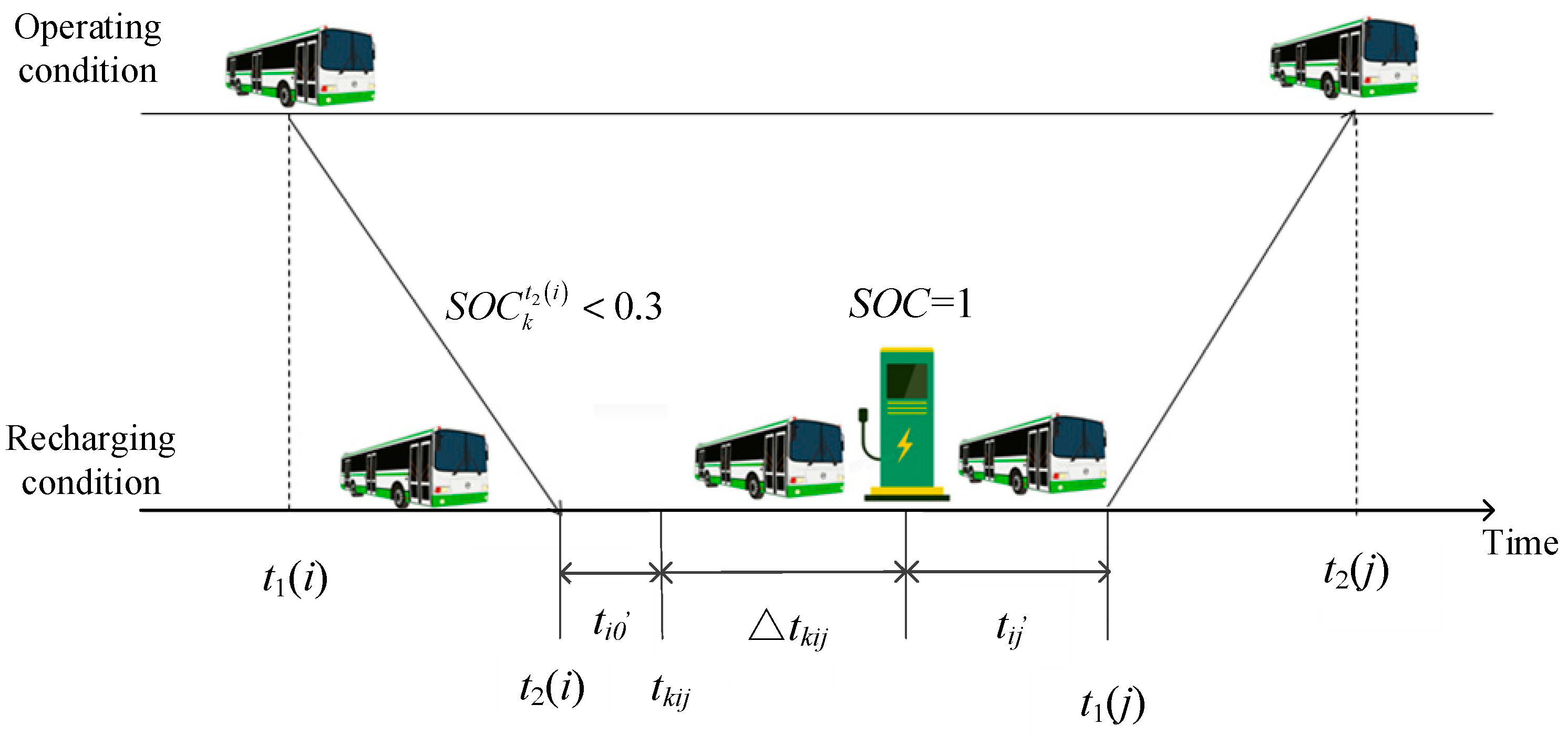
The model takes into account the multi-type EPTVs with different load capacities and battery capacities. Given that maintaining a discharge depth lower than 70–80% can benefit the battery life, it is of significance to control the state of the charge (SOC) of electric vehicles to be above 30%, subject to the battery-allowed mileage. Therefore, when the SOC falls below or equals 30%, the vehicle requires charging. One instance is illustrated in Figure 1. Trip i starts at and ends at , that is, at time , when the SOC is less than 30% and the vehicle starts charging. is the recharging time of vehicle k during the idle time between trip i and trip j.

Figure 1.
Schematic diagram of recharging operation for EPTVs.
3.1. Objective Function
The objective function is to minimize the overall operating cost, which encompasses the following costs: vehicle operation cost (Z1), idle trip cost (Z2), and recharging cost (Z3), respectively. These costs are represented by Equations (1)–(3) and are combined into a single equation, as shown in Equation (4).
where C1, C2, and C3 represent the unit cost of the vehicle operation, the unit cost of an idle trip, and the unit cost of recharging, respectively.
3.2. Constraints
In terms of the multi-type EVS constraints, the idle mileage, charging time, trip connections, and passenger constraints are taken into consideration. In order to cover all trips, Equations (5) and (6) show that each trip is executed only once.
Equation (7) indicates that a vehicle departs from, and eventually returns to, the same depot for the vehicle’s cycle use. Equation (8) ensures that the number of out-flow vehicles does not exceed the total number of available vehicles m0 stored at the depot.
Equation (9) stipulates that the number of passengers allowed to board vehicle k on trip i cannot exceed the maximum capacity of vehicle k assigned to trip i.
where represents the number of passengers of trip i and represents the maximum number of passengers carried by k-th vehicle.
To attain the time compatibility of the trips, Equation (10) guarantees that trip i is executed on time after necessary preparation. The preparation time is calculated using Equation (11).
where depends on whether vehicle k charges or not, and the recharging time is related to the recharging depth.
Referring to the battery discharge data of a bus line [6], we use Equation (12) to identify the relationship between the recharging time and the SOC. The recharging time of an electric vehicle can be calculated using the following equation:
where y represents the recharging depth to clarify the SOC and represents the recharging time, whose unit is hours (h). The battery recharging depth refers to the difference between the energy present during the recharging process and the energy present before recharging.
The battery-allowed mileage constraint based on Equation (13) requires that the driving mileage cannot exceed the maximum battery-allowed mileage of vehicle k.
where the maximum battery-allowed mileage is related to the current discharge depth and the SOC of the vehicle. Jin [6] derived the relationship between the battery-allowed mileage and the discharge depth by fitting the battery discharge data in a bus line. Based on the known specific energy consumption of the battery, the battery-allowed mileage of vehicle k can be calculated by Equation (14).
where a and b are the parameters needed to calibrate according to the specific vehicle type. The values of the battery recharging depth y and the discharge depth x yield to the range [0, 1] and, simultaneously, . The battery recharging depth y is positively related to the recharge time t, while the discharge depth x is positively related to the maximum battery-allowed mileage . The calibration of Equations (12) and (14) refers to the literature [6]. Based on a large number of charging and discharging data of electric buses, the relationship between the recharging depth SOC and the charging time, as well as the relationship between the discharge depth and the maximum battery-allowed mileage, is found.
Considering the energy consumption ratio and the battery capacity ratio between single large-type or single small-type and single medium-type vehicles, Equation (14) is used to fit the monitoring data. Then, we derive the relationship in Equation (15) between the battery-allowed mileage and the discharge depth for single a large-type vehicle and a single small-type vehicle.
where represents the battery-allowed mileage of the vehicle and x represents the discharge depth.
4. Solution Algorithm
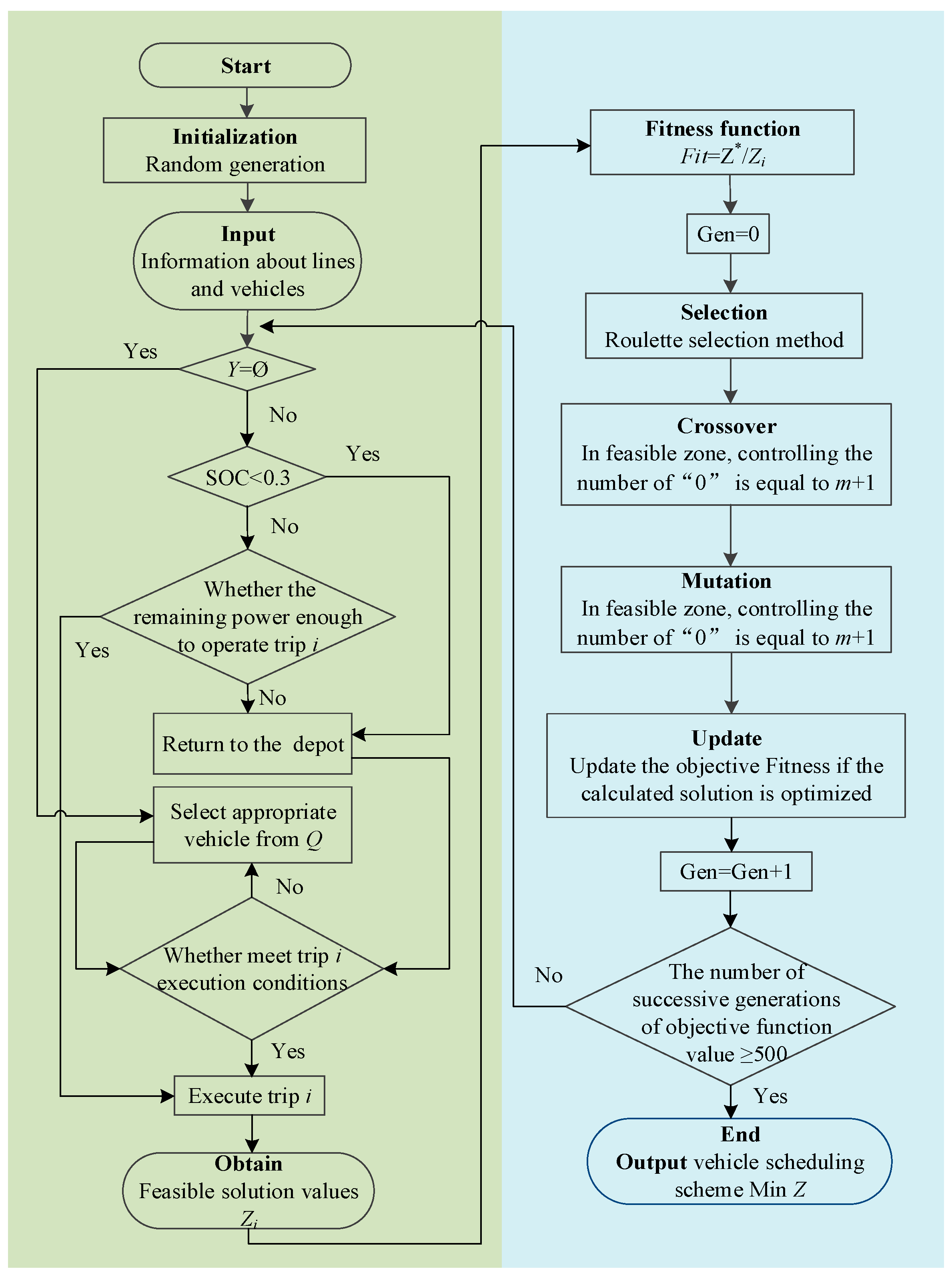
In this section, we utilize the genetic algorithm (GA) to solve the multi-type EVS model. It is important to note that one feasible solution used in GA is derived from a preprocessing procedure (Section 4.1). Section 4.2 iteratively updates the feasible solution set until matching the termination condition by the utilization of GA. Otherwise, we need to test the new feasible solutions (from Section 4.1) by the use of that shown in Section 4.2.
4.1. Preprocessing Procedure
Here, we take one certain vehicle scheduling scheme as one example. Suppose that the total number of trips is n and the number of vehicles stored in the depots is m. The execution conditions for trip i are as follows: for vehicle k, if , i.e., the vehicle has sufficient capacity and enough energy to complete the trip and return to the depot. In addition, trip i should be executed on time. After the above conditions are met, vehicle k can execute trip i, that is, . The following details the feasible solution generation process:
Step 1: If , select the vehicle from set Y to execute trip i. If the vehicle (k) that has completed trip a meets the conditions for trip i execution, set and go to Step 2. Otherwise, if , go to Step 4.
Step 2: If the of vehicle k is less than 0.3, it means that the vehicle needs to return to the depot for recharging. After being fully charged, if the condition of executing trip i is met, then execute Step 1.
Step 3: If the , and the remaining energy of the vehicles in Y is enough to operate trip i, assign vehicle k in Y to execute trip i. Otherwise, if the remaining energy of all of the vehicles in Y cannot execute any trip, then the vehicle needs to return to the depot to charge as well, and if the condition of executing trip i is met after charging, execute Step 1.
Step 4: If the condition of executing trip i still cannot be satisfied, or , select a vehicle from Q that satisfies the condition of executing trip i to perform trip i.
Step 5: Repeat Steps 1–4 for each trip until all of the trips have been assigned. Then, output the feasible solution Zi.
4.2. Genetic Algorithm
The vehicle scheduling solution can output a series of trip assignments to obtain the trip chain of vehicles. The GA is a population-based optimization search algorithm that uses the survival of the fittest [20]. To tackle this problem, we employ the GA to encode the execution assignment for each trip. Primarily, we input the relevant information about the routes and vehicles involved, including the line mileage, the number of vehicles, the vehicle idle mileage, and so on. Next, we arrange the trips in ascending order based on their departure times. The steps involved with GA are exhibited below, as follows:
- (1)
- Encoding
Every feasible solution is encoded into a chromosome with length m + n + 1. Here, m is the number of all vehicles stored in the depot, n is the number of trips, and 1 refers to the space. For example, a chromosome can be written as follows:
where 0 denotes the depot and represents vehicle k operating for trip j. The following vector (0, 1, 5, 7, 0, 4, 8, 0, 2, 3, 0, 6, 0, 0) represents the vehicle scheduling scheme, which means that there are eight service trips to execute overall, and the fleet size in the depot is five:
- Vehicle 1: Depot → Trip 1 → Trip 5 → Trip 7 → Depot
- Vehicle 2: Depot → Trip 4 → Trip 8 → Depot
- Vehicle 3: Depot → Trip 2 → Trip 3 → Depot
- Vehicle 4: Depot → Trip 6 → Depot
- Vehicle 5: No trip to operate
- (2)
- Initialization
Initialization is the primary step of the GA, in which the individuals required (i.e., an initial population with length m + n + 1) are generated by a uniform random number generator. Note that there is no repeated initial population generated. Ultimately, an NP × (m + n + 1) matrix is formed, where NP is the number of initial populations. The more variables in the GA, the larger the initial population is. Primarily, the population numbers are tested by several experiments. We set the initial population numbers (NP) in Section 5.2.1, Section 5.2.2 and Section 5.2.3, which are 50, 100, and 150, respectively.
- (3)
- Fitness function
According to a multi-objective nonlinear optimization model with many constraints, we assign different weights to three sub-objectives and deal with the constraints by introducing a penalty parameter M.
The fitness function is obtained by linear scaling of objective Z.
where corresponds to the optimized genotype in the current population and is the objective value of the i-th genotype. We use the fitness function to assess the improvement of each (solution) genotype.
- (4)
- Selection
According to the fitness function of an individual, as well as certain rules or methods, some excellent individuals outperforming from population P(t) of generation t are selected and passed to the next generation P(t + 1) by the Roulette selection method. If the fitness function of individual i is Fi, and the population size is NP, the selection probability can be expressed as follows:
- (5)
- Crossover
The crossover process is carried out to pair two individuals that are randomly selected and to decide whether to cross based on the predefined crossover probability (which is usually equal to 1). Considering a number x, which is randomly generated in [0, 1], if , then a crossover is performed. Each individual selected from population P(t) is randomly matched, and part of the chromosomes between each pair of individuals is exchanged with crossover probability . In this paper, we adopt the sequential crossing and take .
- (6)
- Mutation
Mutation is a random process that refers to one allele on the chromosome being replaced by another to generate a new genetic structure with mutation probability . The mutation probability generally ranges in [0.001, 0.1]. We set and mutate in the way of an insert mutation, that is, we randomly select a trip and insert it into a random position. For real-number mutation, the corresponding gene value is replaced with other random values within the range of values.
- (7)
- Termination criterion
When the objective function value is continuously stable at 500 generations of iterations, GA stops updating and outputs the optimized solution.
The flowchart of GA is presented in Figure 2.
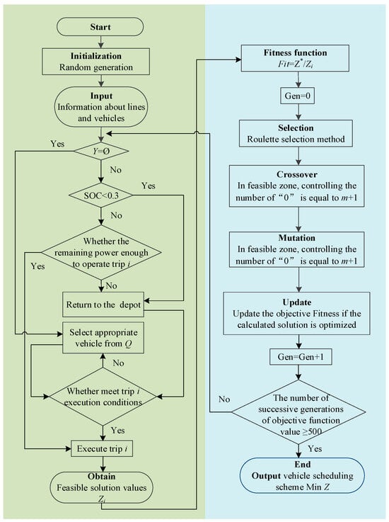
Figure 2.
Flowchart of the solution algorithm.
5. Case Study
5.1. Data and Parameter Settings
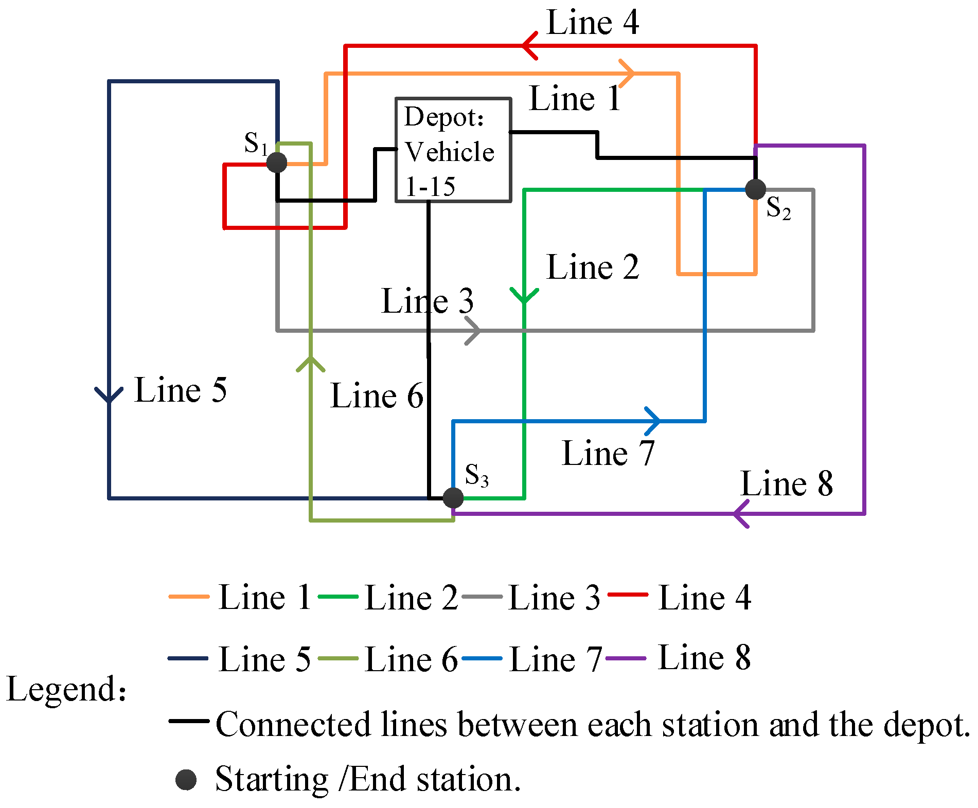
This section depicts how to use the proposed EVS model as per each case. Primarily, an initial timetable is provided. There is a stipulation that all of the EPTVs in the depot must complete the previous trip before proceeding to the next step. The experimental scenario consists of eight lines and one depot, as illustrated in Figure 3. S1 is the starting station of lines 1, 3, and 5 and also is the terminal station of lines 4 and 6. S2 is the starting station of lines 2, 4, and 8, and meanwhile is also the terminal station of lines 1, 3, and 7. S3 is the starting station of lines 6 and 7, and simultaneously is the terminal station of lines 2, 5, and 8. These 8 lines, each with 3 trips, each half an hour apart, make a total of 24 trips. The first eight trips correspond to the first trip of eight lines, respectively. Trip 9–16 is postponed for half an hour on the basis of the first trip, that is, trip 9–16 corresponds to the second trip of line 1–8, respectively, and trip 17–24 corresponds to the third trip of line 1–8, respectively.
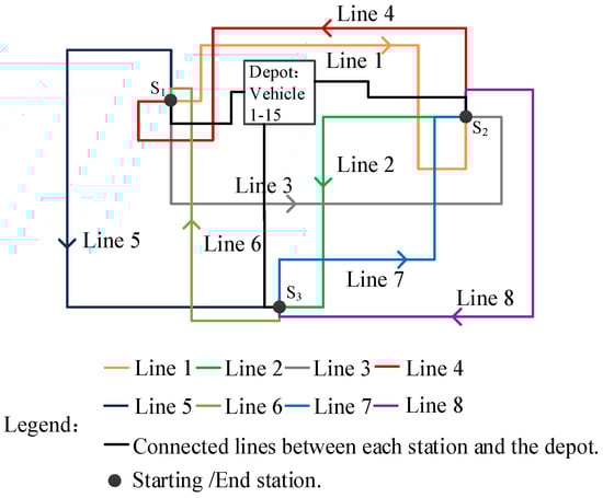
Figure 3.
The layout of lines.
As per Assumption (1), the charging infrastructure is situated within the depot. We stipulate five vehicles as the minimum fleet size to be stored in the depot. The schedule of the start and end times for each trip is provided in Table 3. The corresponding idle mileage for the eight trips is demonstrated in Table 4. Table 5 shows the idle connection time between each line. Table 6 shows the mileage of each line. Table 7 shows the comparison of parameters for each vehicle type.
Table 3.
Schedule of departure and end times for trip 1–8.
Table 4.
Idle mileage of connection between each line (km).
Table 5.
Idle time of connection between each line (min).
Table 6.
Mileage of each line (km).
Table 7.
Comparison of each type of vehicle.
We specify the trip and its sequence performed by the k-th vehicle in the coding. For instance, a feasible solution can be represented by a GA-style result with a length of 5 + 8 + 1. Herein, “5” refers to the number of vehicles, “8” represents the number of trips, and “1” is the space, respectively.
In order to ensure the health of the battery, we stipulate that the maximum discharge depth of the electric vehicle during operation is limited to 70%. When a battery possesses a discharge depth of 70%, the maximum battery-allowed mileage for the large-type, medium-type, and small-type vehicles can be determined by Equation (15) as 106 km, 85 km, and 75 km, respectively. In other words, the percentage of remaining energy, i.e., the SOC, for all of the vehicles before they complete their trips and return to the depot is greater than 30%. The unit of the SOC is percentage.
5.2. Result Analysis
Based on the above scenario-based parameter settings, the vehicle scheduling and recharging scheduling of the EPTVs for the eight lines are optimized as per the model. The algorithm solution is coded in Matlab R2018a. The outcome from the model is computed on one personal computer with Intel ®core™ i5-11400H CPU 16G RAM. The performance and comparisons of single-one-type, two-type, and multi-type vehicle scheduling schemes will be analyzed in Section 5.2.1, Section 5.2.2 and Section 5.2.3.
5.2.1. Scenario 1: One-Trip Frequency Scenario
Scenario 1 shows that only one trip is deployed for each line. This scene corresponds to the commuting service connection between the outer suburbs and downtown. One trip is provided hourly. In general, the passenger demand is not large. The number of passengers per trip is shown in Table 8.
Table 8.
The number of passengers on each trip in Scenario 1.
- (1)
- Single-one-type vehicle scheduling
Subject to the maximum load capacity constraint shown in Equation (9), only large-type vehicles are capable of meeting the demand for each trip. Therefore, the fleet size yields to only the large-type vehicles. The performance of the results is estimated by means of the operation cost (Z1), idle mileage (Z2), and recharging time (Z3).
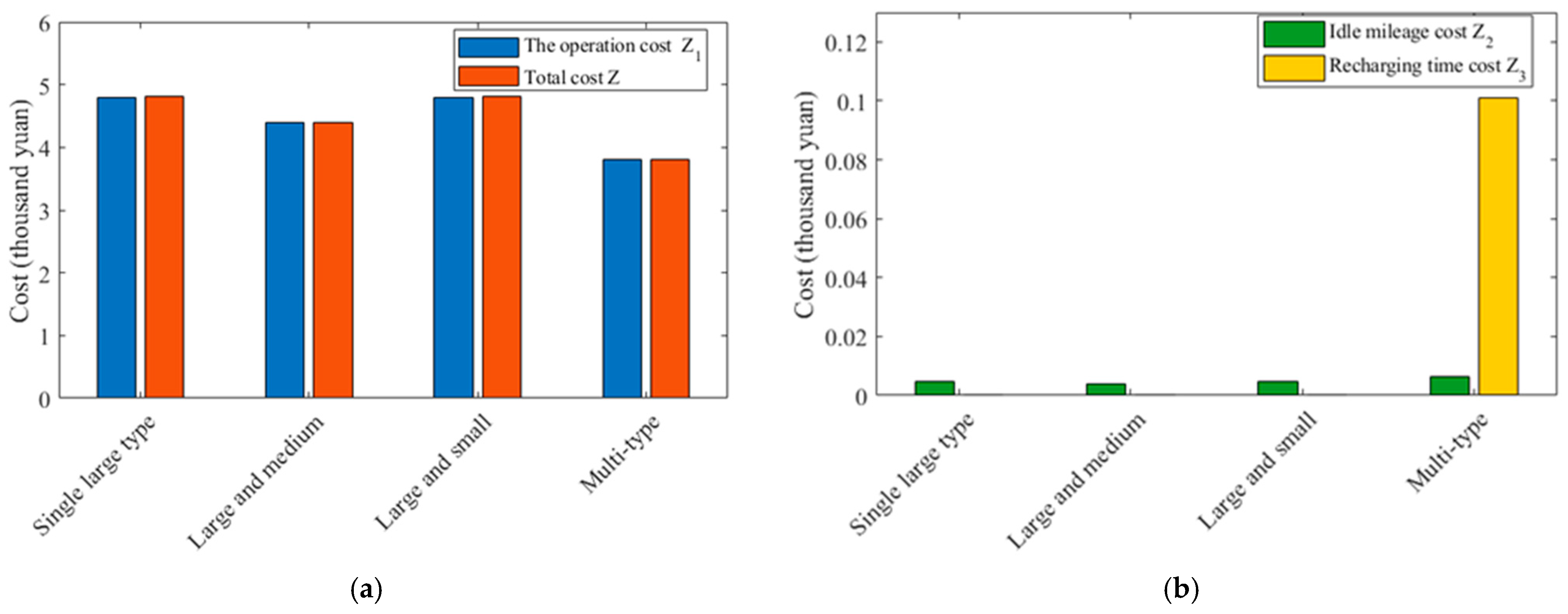
Four physical vehicles are utilized to complete these eight trips. The results reveal that the operation cost is CNY 4.8047 thousand. The idle mileage is 47 km, incurring a cost of CNY 0.0047 thousand. The total recharging time is 0, and, consequently, the recharging cost is CNY 0. The optimized solution obtained through the GA is represented as (0 4 6 0 1 5 0 2 7 0 0 3 8 0), which can be interpreted by Table 9 and Table 10.
Table 9.
Trip chain of single-type vehicle scheme.
Table 10.
Objectives of single-type vehicle scheme in Scenario 1 (CNY thousand).
- (2)
- Two-type vehicle scheduling
In terms of the two-type vehicle scheduling problem, Table 11 and Table 12 demonstrate the compositional type scheme through cost comparisons Z1, Z2, and Z3, respectively. Two resultant schemes (the 2nd and 3rd schemes) are derived. Because of the given passenger demand, the large-type vehicle is necessary. That is, the 2nd scheme refers to the combination of large and medium vehicles, in which the load capacities are 60, 80, 80, and 60, respectively. The 3rd scheme includes large and small types, where the load capacities are 80, 40, 40, 80, and 40, respectively.
Table 11.
Trip chain of the two-type vehicle schemes.
Table 12.
Objectives of two-type vehicle schemes (CNY thousand).
By examining Table 11 and Table 12, we can observe that the idle mileage of the 2nd scheme (including two large vehicles and two medium vehicles) is 39 km, which is 8 km less than the 3rd scheme (including two large vehicles and three small vehicles). Compared with the 3rd scheme, the number of vehicles used in the 2nd scheme is reduced by one, and the operation cost is reduced by CNY 0.4 thousand. The total cost is reduced by about 8.3%. Furthermore, it is noteworthy that neither of the schemes require any recharging events.
- (3)
- Multi-type vehicle scheduling
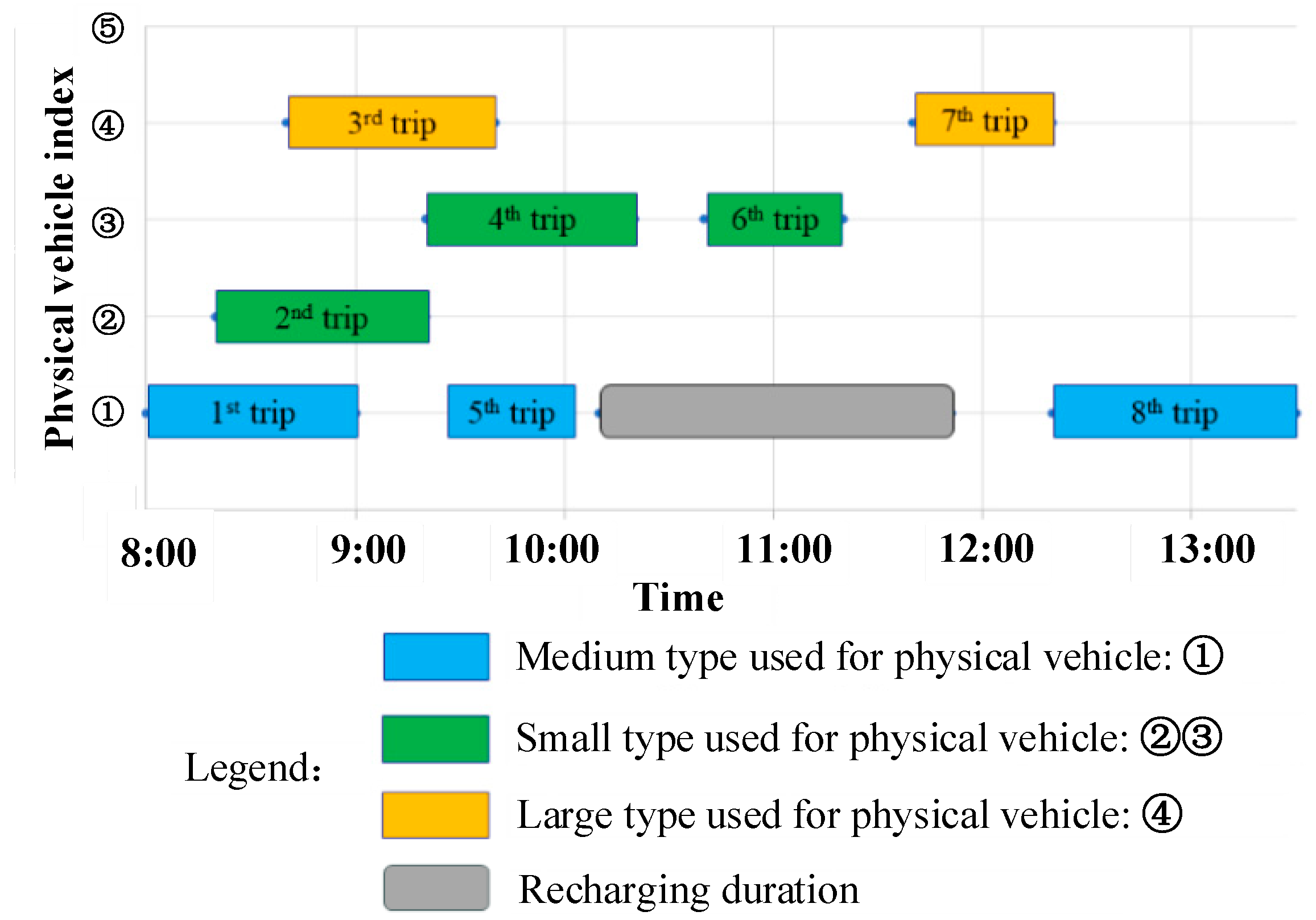
A fleet of four multi-type vehicles is utilized, resulting in an operation cost of CNY 3.8075 thousand. The idle mileage is 65 km, incurring a cost of CNY 0.0065 thousand. The total recharging time amounts to 1.68 h, with a corresponding recharging cost of CNY 0.101 thousand. The final EVS is presented in Figure 4. It is worth noting that the number of vehicles departing from the depot corresponds to the number of vehicles returning after completing all of the trips, with no scheduling conflicts, and in compliance with the required pure EVS criteria. The output vehicle scheme is (60, 40, 40, 80), representing the utilization of medium-type, small-type, small-type, and large-type vehicles, respectively. The optimized solution obtained with the GA is represented as (0, 1, 5, 8, 0, 2, 0, 4, 6, 0, 3, 7, 0, 0). The trip chain of the multi-type scheme is demonstrated in Table 13. The results are generated for comparison in Table 14.
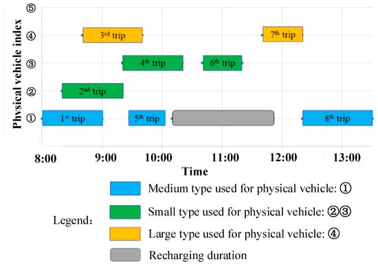
Figure 4.
Electric vehicle scheduling with recharging process.
Table 13.
Trip chain of the multi-type vehicle scheme.
Table 14.
Comparison of four schemes (CNY thousand).
In order to show how to determine the recharging events, we give a detailed example below, as follows:
Physical Vehicle ①: When Vehicle ① departs from the depot to operate the 1st trip, its mileage is calculated as 3 + 30, which is less than 85 km, indicating that no recharging is needed. If Vehicle ① continues to run the 5th trip, the accumulated mileage becomes 3 + 30 + 7 + 20, which is still less than 85 km, and no charging is required. However, if Vehicle ① proceeds to operate the 8th trip and returns to the depot, the accumulated mileage becomes 3 + 30 + 7 + 20 + 9 + 40 + 5, which exceeds 85 km. Therefore, Vehicle ① needs to return to the depot for recharging before the 8th trip. The mileage required to return to the depot after the 5th trip is calculated as 3 + 30 + 7 + 20 + 5 = 65 km. As per Equation (15), we can determine that the discharge depth at this point is 53.54%. Additionally, using Equation (12), the recharging time is found to be 1.68 h, approximately 101 min. After recharging, the start time for the 8th trip is calculated as 10:00 + 10 min + 101 min + 8 min = 11:59, which is before the original start time of the 8th trip (12:20). Hence, the time condition is met. Consequently, the actual idle mileage for Vehicle ① is 3 + 7 + 5 + 4 + 5 = 24 km.
Physical Vehicle ②: When Vehicle ② departs from the depot for the 2nd trip, the traveled mileage is calculated as 4 + 40 + 5, which is less than 75 km, indicating that no recharging is required. The idle mileage for Vehicle ② is 4 + 5 = 9 km.
Physical Vehicle ③: When Vehicle ③ performs the 4th trip, the traveled mileage is calculated as 4 + 30, which is less than 75 km, indicating that no recharging is needed. If Vehicle ③ continues to operate the 6th trip and then returns to the depot, the accumulated mileage becomes 4 + 30 + 8 + 20 + 4, which is still less than 75 km. Therefore, Vehicle ③ can complete all of the assigned trips without requiring charging during execution. The idle mileage for Vehicle ③ is 4 + 8 + 4 = 16 km.
The mileage for Vehicle ④ during the 3rd trip is calculated as 3 + 30, which is less than 106 km, indicating that no recharging is required. Additionally, when Vehicle ④ continues to run the 7th trip and returns to the depot, the accumulated mileage remains below 106 km, calculated as 3 + 30 + 9 + 40 + 4. Therefore, Vehicle ④ does not need to return to the depot for recharging. The idle mileage for Vehicle ④ is 3 + 9 + 4 = 16 km. On the other hand, Vehicle ⑤ does not have any assigned trips.
By comparing the four vehicle schemes, it becomes evident that the total cost is significantly reduced by about 21% compared with the single large vehicle scheme when employing multi-type vehicles. This highlights the importance and benefits of studying multi-vehicle approaches for pure EVS.
For Scenario 1, the cost of the four vehicle schemes is illustrated in Figure 5.
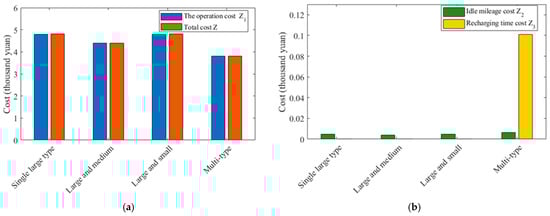
Figure 5.
Comparison of the cost among various vehicle schemes under a 1-trip frequency scenario: (a) Comparison of operation cost Z1 and total cost Z and (b) Comparison of idle mileage cost Z2 and recharging time cost Z3.
The 4th scheme demonstrates its ability to efficiently accommodate a high passenger demand with a minimum total cost (CNY 3.8075 thousand), as indicated in Table 14. However, this multi-type scheme has a higher idle mileage, due to the additional recharging scheduling. Its cost associated with idle mileage constitutes a minor portion of the total cost, exerting a minimal impact.
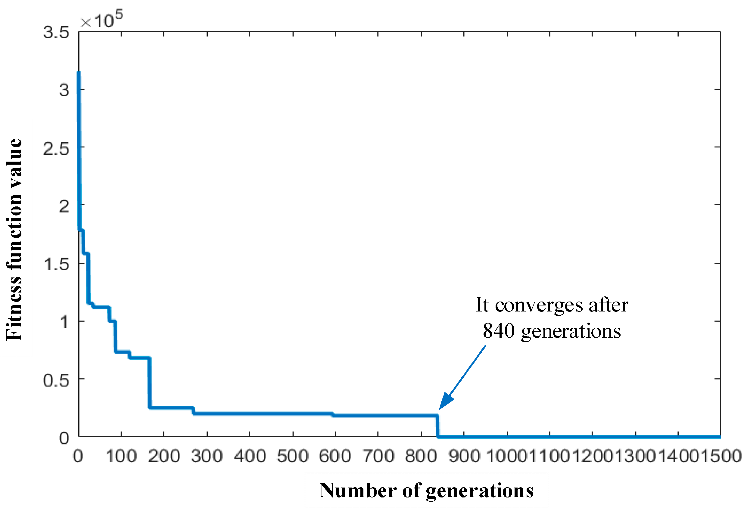
The convergence of the feasible solution is mirrored in Figure 6. The average fitness function value gradually decreases over time, indicating the optimization process. The evolutionary progress exhibits rapid improvements within the first 100 generations, followed by a slower rate of improvement between 100 and 840 generations. Eventually, the fitness values stabilize after 840 generations. This convergence terminates at 3.8075. This demonstrates the effectiveness of the solution and its ability to derive the optimized value.
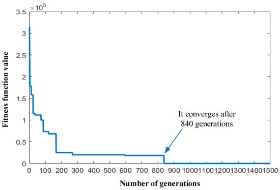
Figure 6.
The convergence curve of the fitness value in Scenario 1.
5.2.2. Scenario 2: Two-Trip Frequency Scenario
Scenario 2 shows that two trips are deployed for each line. The departure interval of the PT service is half an hour. The number of passengers per trip is shown in Table 15.
Table 15.
The number of passengers on each trip in Scenario 2.
A performance comparison of the seven schemes is given in Table 16. The comparable categories include (1) single-one-type VS, (2) two-type VS, and (3) multi-type VS. In detail, Category (1) refers to the 1st, 2nd, and 3rd scheme. Category (2) has the 4th, 5th, and 6th scheme. Category (3) is the 7th scheme.
Table 16.
Comparison of 7 schemes in Scenario 2 (CNY thousand).
- (1)
- Single-one-type vehicle scheduling scheme
If the capacity of the first vehicle cannot accommodate all of the passengers, some of the passengers have to be left behind and wait for the next vehicle. Considering only one type of vehicle, the results of three single-type schemes in Scenario 2 are shown in Table 17.
Table 17.
Objectives of single-type vehicle scheme in Scenario 2 (CNY thousand).
The 1st scheme (single large-type): Eight electric vehicles are utilized, resulting in an operation cost of CNY 9.6103 thousand. The idle mileage is 88 km, with an associated cost of 0.0088 CNY thousand. The total recharging time is 1.5 h, with a recharging cost of CNY 0.0015 thousand. The optimized solution obtained through the GA is represented as (0 11 0 3 8 0 0 1 13 14 0 12 7 0 5 6 0 2 0 9 4 15 0 10 16 0 0).
The 2nd scheme (single medium-type): Similar to the large-type vehicle scenario, eight electric vehicles are employed, resulting in an operation cost of CNY 8.0111 thousand. The idle mileage is 96 km, with a cost of CNY 0.0096 thousand. The total recharging time is 1.5 h, with a recharging cost of CNY 0.0015 thousand. The optimized solution derived through the GA is represented as (0 11 6 0 13 7 0 10 0 1 4 0 5 14 16 0 0 2 0 0 3 12 15 0 9 8 0).
The 3rd scheme (single small-type): Ten electric vehicles are utilized, resulting in an operation cost of CNY 8.0100 thousand. The idle mileage is 85 km, with a cost of CNY 0.0085 thousand. The total recharging time is 1.5 h, with a recharging cost of CNY 0.0015 thousand. The optimized solution derived through the GA is represented as (0 1 12 16 0 10 14 0 15 0 2 13 6 0 4 0 3 0 8 0 11 0 5 7 0 9 0).
- (2)
- Two-type vehicle scheduling
In the 4th scheme—i.e., the large- and medium-type combination scheme, eight EPTVs are utilized, in which three are large- while the other five are medium-sized. The operation cost amounts to CNY 8.6097 thousand. The idle mileage reaches 85 km, incurring a cost of 0.0083 CNY thousand. The total recharging time is 1.4 h, with a corresponding cost of CNY 0.0014 thousand. The optimized solution obtained is represented as (0 1 4 0 0 0 10 15 0 2 14 0 5 7 0 9 12 0 11 8 0 13 0 3 6 16 0).
In the 5th scheme, in which large and small types are synthesized, eight EPTVs are used, consisting of four large- and four small-type vehicles. The operation cost is CNY 8.0111 thousand. The idle mileage amounts to 97 km, incurring a cost of CNY 0.0097 thousand. The total recharging time is 1.4 h, with a corresponding cost of CNY 0.0014 thousand. The optimized solution derived is represented as (0 1 5 8 0 2 0 13 7 0 0 10 15 0 9 16 0 4 14 0 11 6 0 0 3 12 0).
In the 6th scheme, in which medium and small types are synthesized, 10 EPTVs are employed, with 5 medium- and 5 small-type vehicles. The operation cost amounts to CNY 9.0131 thousand. The idle mileage reaches 97 km, incurring a cost of CNY 0.0112 thousand. The total recharging time is 1.9 h, with a corresponding cost of CNY 0.0019 thousand. The optimized solution obtained is represented as (0 9 8 0 13 0 2 4 15 0 5 0 7 0 1 0 12 0 3 6 0 10 14 0 11 16 0).
- (3)
- Multi-type vehicle scheduling
In the 7th scheme (i.e., multi-type), a total of 10 electric vehicles are utilized, comprising 3 large-type vehicles, 3 medium-type vehicles, and 4 small-type vehicles. The operation cost amounts to CNY 9 thousand. The idle mileage reaches 79 km, incurring a corresponding cost of CNY 0.0079 thousand. The total recharging time is 0 h, resulting in no recharging cost. The optimized solution derived through the GA is represented as (0 12 7 0 2 15 0 13 0 11 16 0 9 6 0 1 0 4 0 5 14 0 10 0 3 8 0).
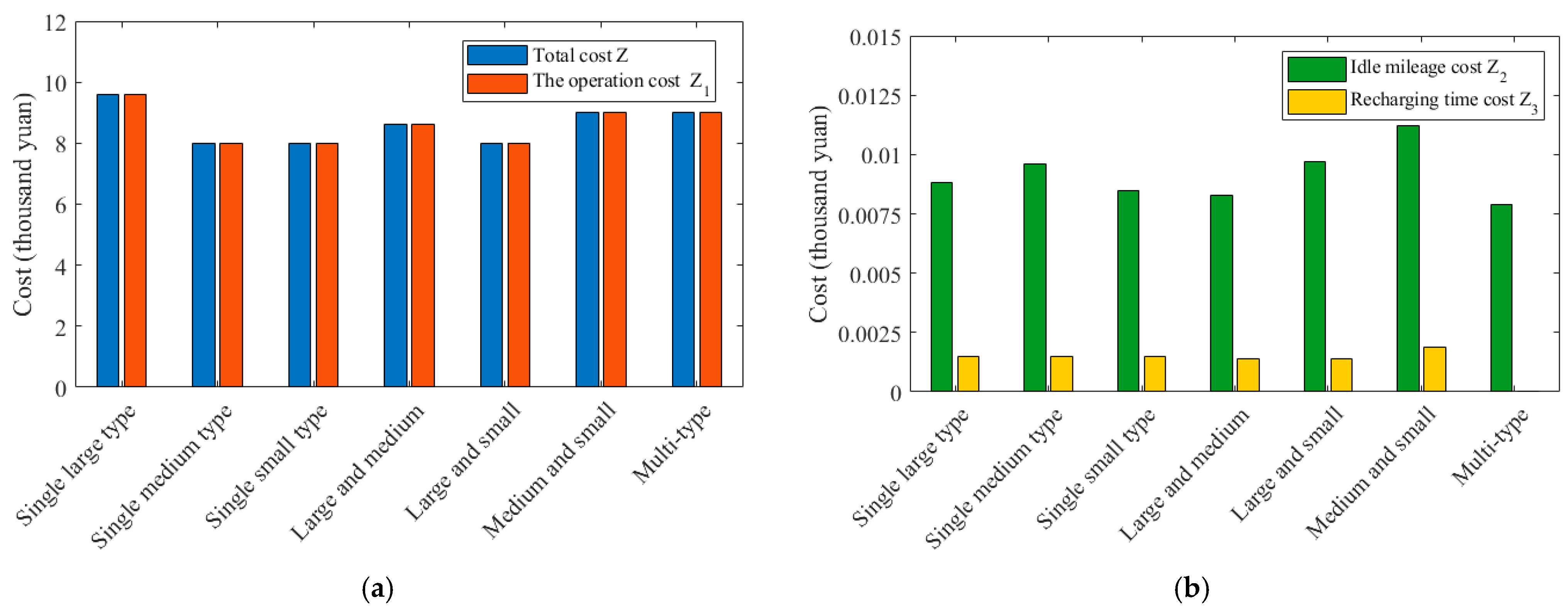
For Scenario 2, the cost of the seven vehicle schemes is illustrated in Figure 7.

Figure 7.
Comparison of the cost among various vehicle schemes under a 2-trip frequency scenario: (a) Comparison of operation cost Z1 and total cost Z and (b) Comparison of idle mileage cost Z2 and recharging time cost Z3.
5.2.3. Scenario 3: Three-Trip Frequency Scenario
Scenario 3 shows that three trips are deployed for each line. The departure interval is 30min/trip. The number of passengers per trip is shown in Table 18.
Table 18.
The number of passengers on each trip in Scenario 3.
A performance comparison of the seven schemes is given in Table 19. The comparable categories include (1) single-one-type VS, (2) two-type VS, and (3) multi-type VS. In detail, Category (1) refers to the 1st, 2nd, and 3rd scheme. Category (2) shows the 4th, 5th, and 6th scheme depicted. Category (3) shows the 7th scheme.
Table 19.
Comparison of the 7 schemes in Scenario 3 (CNY thousand).
- (1)
- Single-one-type vehicle scheduling
If the capacity of the previous vehicle cannot accommodate all of the passengers, some of the passengers must be left to wait for the next vehicle. Considering only one vehicle type, the results of three single-type schemes in Scenario 3 are shown in Table 20.
Table 20.
Objectives of single-type vehicle scheme in Scenario 3 (CNY thousand).
The 1st scheme (single large-type): Eleven electric vehicles are utilized, resulting in an operation cost of CNY 13.2202 thousand. The idle mileage reaches 157 km, incurring a cost of CNY 0.0157 thousand. The total recharging time is 4.5 h, with a corresponding cost of CNY 0.0045 thousand. The optimized solution derived through the GA is represented as (0 14 7 24 0 0 20 0 18 21 23 0 0 4 8 0 2 5 15 0 0 3 16 0 1 11 22 0 9 12 0 17 13 0 0 10 6 0 19 0).
The 2nd scheme (single medium-type): A total of 13 electric vehicles are utilized. The operation cost amounts to CNY 13.0244 thousand. The idle mileage reaches 167 km, incurring a cost of CNY 0.0167 thousand. The total recharging time is 3 h, resulting in a recharging cost of CNY 0.0030 thousand. The optimized solution obtained through the GA is represented as (0 2 21 15 0 10 13 0 18 5 24 0 1 19 0 12 23 0 22 0 20 0 4 0 9 7 0 14 16 0 0 11 8 0 3 0 17 6 0 0).
The 3rd scheme (single small-type): A total of 15 electric vehicles are used. The operation cost amounts to CNY 12.0154 thousand. The idle mileage reaches 150 km, incurring a cost of CNY 0.0150 thousand. The total recharging time is 4 h, resulting in a recharging cost of CNY 0.0040 thousand. The optimized solution obtained is represented as (0 2 6 0 10 14 0 18 0 17 0 19 24 0 1 5 0 4 0 13 0 3 23 0 11 0 12 0 9 22 16 0 21 7 0 15 0 20 8 0).
- (2)
- Two-type vehicle scheduling
In the 4th scheme—i.e., the large- and medium-type combination scheme, a total of 12 EPTVs are used, consisting of 5 large- and 7 medium-type vehicles. The operation cost amounts to CNY 13.0187 thousand. The idle mileage reaches 151 km, incurring a cost of CNY 0.0151 thousand. The total recharging time is 3.6 h, with a corresponding cost of CNY 0.0036 thousand. The optimized solution obtained through the GA is represented as (0 3 8 0 10 15 0 4 22 0 0 12 0 0 18 23 0 17 24 0 9 13 16 0 20 14 7 0 19 6 0 5 0 1 11 0 2 21 0 0).
In the 5th scheme, in which large and small types are synthesized, a total of 13 electric vehicles are utilized, comprising 7 large- and 6 small-type vehicles. The operation cost amounts to CNY 11.8219 thousand. The idle mileage reaches 161 km, incurring a cost of CNY 0.0161 thousand. The total recharging time is 4.1 h, resulting in a recharging cost of CNY 0.0041 thousand. The optimized solution obtained is represented as (0 13 23 0 11 14 0 19 0 1 7 0 9 15 0 2 5 6 0 12 0 4 24 0 0 18 16 0 0 20 0 17 21 0 10 8 0 3 22 0).
In the 6th scheme (medium- and small-type), a total of 14 electric vehicles are used, with 6 medium- and 8 small-type vehicles. The operation cost amounts to CNY 13.6218 thousand. The idle mileage reaches 156 km, incurring a cost of CNY 0.0156 thousand. The total recharging time is 6.2 h, with a corresponding cost of CNY 0.0062 thousand. The optimized solution obtained is represented as (0 13 22 0 1 5 8 0 6 15 0 0 20 0 4 16 0 18 23 0 3 0 12 0 11 0 10 0 19 7 0 9 21 0 17 24 0 2 14 0).
- (3)
- Multi-type vehicle scheduling
In the 7th scheme (i.e., multi-type), a total of 12 electric vehicles are used, with 4 large-type vehicles, 4 medium-type vehicles, and 4 small-type vehicles. The operation cost amounts to CNY 12.0213 thousand. The idle mileage reaches 150 km, incurring a cost of CNY 0.0150 thousand. The total recharging time is 6.3 h, with a corresponding cost of CNY 0.0063 thousand. The optimized solution derived through the GA is represented as (0 0 19 0 5 0 2 6 0 11 23 0 0 10 13 0 4 0 3 8 0 9 21 0 14 7 24 0 0 1 12 0 17 20 15 0 18 22 16 0). For Scenario 3, the cost of the seven vehicle schemes is illustrated in Figure 8.
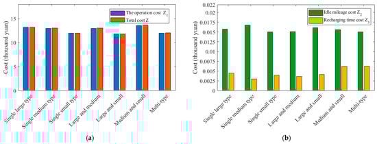
Figure 8.
Comparison of the cost among various vehicle schemes under a 3-trip frequency scenario: (a) Comparison of operation cost Z1 and total cost Z and (b) Comparison of idle mileage cost Z2 and recharging time cost Z3.
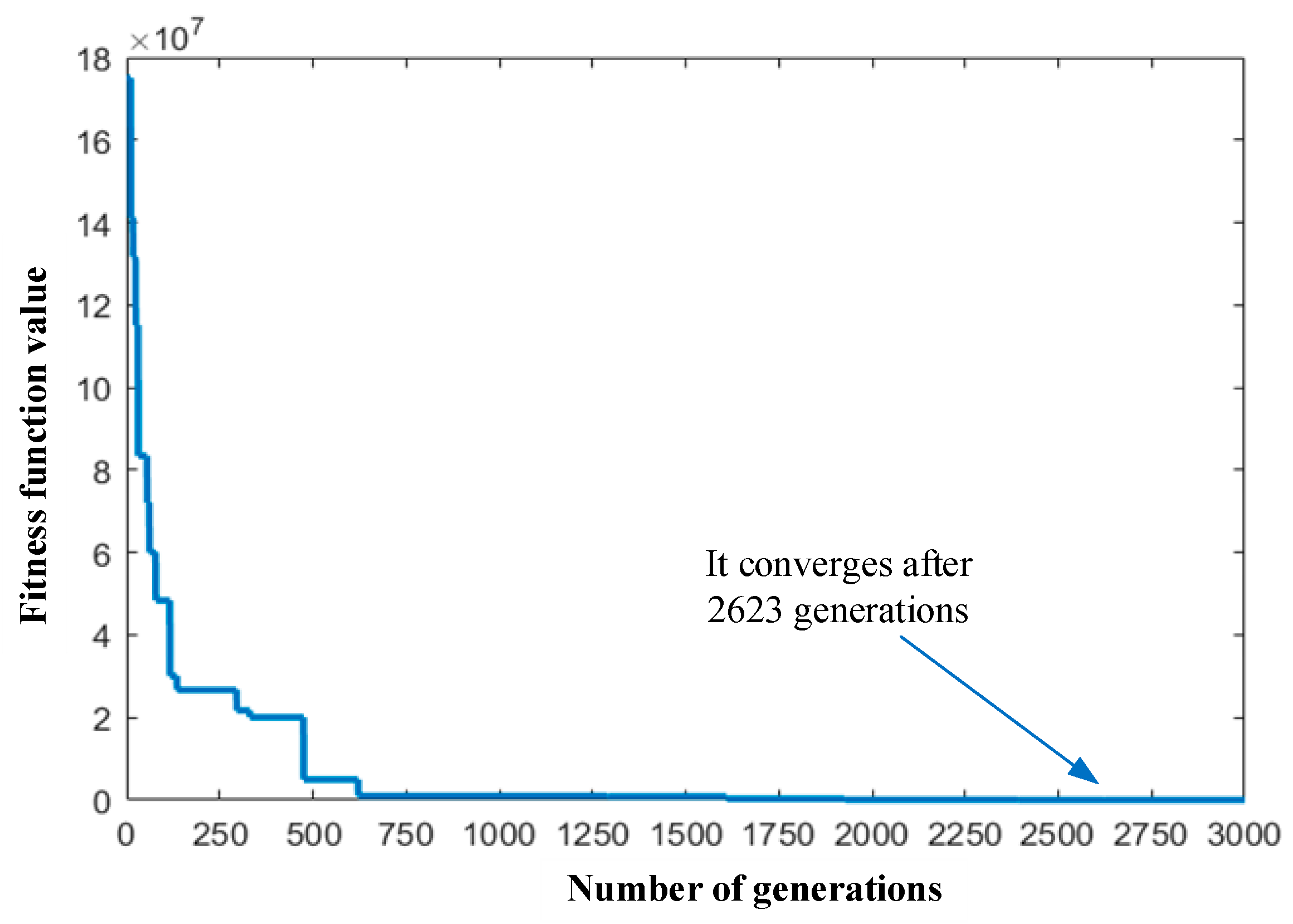
The feasibility of the solution is demonstrated in Figure 9. It shows that the fitness function of the GA converges. The average fitness function value gradually decreases, prior to the 500th generation. The evolutionary progress exhibits a rapid decrease in the early stages, before 500 generations, followed by a slower decline between 500 and 2623 generations. As the generations progress, the fitness values stabilize and eventually approach the optimized value after 2623 generations. This indicates that GA is able to find an optimized solution for the case.

Figure 9.
Convergence curve of the fitness value in Scenario 3.
We compared the total cost of each line optimization scheme with the total cost of the 1st scheme (single large-type), as illustrated in Figure 10. The results clearly indicate that the implementation of multi-type vehicles can significantly reduce the costs. In the case of Scenario 1, the two-type vehicle scheme demonstrates an 8.3% reduction in the total cost compared to the 1st scheme (single large-type), while the 7th scheme (multi-type) achieves a remarkable 20.7% reduction. Similarly, for Scenario 2, the total cost of the 7th scheme (multi-type) is 6.2% lower than that of the 1st scheme (single large-type), and the two-type vehicle scheme achieves a 10.6% reduction. As for Scenario 3, the 7th scheme (multi-type) yields a 9.1% cost reduction compared to the 1st scheme (single large-type), and the two-type vehicle scheme reduces the total cost by up to 10.6% compared with the 1st scheme (single large-type). While the 3rd scheme (single small-type) also reduces the total cost in Scenario 2 and 3, it unfortunately leaves a significant number of passengers delayed—32 passengers in Scenario 2 and 54 passengers in Scenario 3. Therefore, the application of multi-type vehicles proves to be a superior solution.
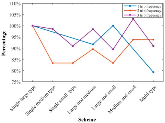
Figure 10.
Total cost percentage of each scheme compared to single large-vehicle-type scheme.
5.3. Sensitivity Analysis
We set different weight coefficient values of C1 (unit: CNY thousand/vehicle), C2 (unit: CNY thousand/km), and C3 (unit: CNY thousand/h) to conduct a sensitivity analysis. The values of C1, C2, and C3 are chosen from 1, 0.001 and 0.0001, yielding a total of seven different scenario combinations corresponding to the seven distinct schemes in Table 21. For each scenario, we compute the cost of the operation of the vehicles, the idle mileage, and the recharging time for seven proposed schemes under a three-trip frequency scenario. By comparing the total cost, we investigate the saving percentage. The specific values are shown in Table 21.
Table 21.
The performance of the different scenarios.
Schemes 1–7 in Table 21 correspond to the seven schemes presented in Section 5.2, respectively, as follows:
- Scheme 1: single large-type vehicle;
- Scheme 2: single medium-type vehicle;
- Scheme 3: single small-type vehicle;
- Scheme 4: large- and medium-type vehicle;
- Scheme 5: large- and small-type vehicle,
- Scheme 6: medium- and small-type vehicle;
- Scheme 7: multi-type vehicle.
In observing the seven scenarios, we find that, in Scenarios I, III, VI, and VII, Scheme 1 has the lowest total cost, while Scheme 3 has the highest total cost. In Scenario II, Scheme 4 has the lowest total cost, while Scheme 3 has the highest total cost. In Scenarios IV and V, Scheme 7 has the lowest total cost, while Scheme 3 has the highest total cost. Since Schemes 1, 4, and 7 are likely to have the lowest total cost, different scenarios need to be analyzed in order to determine their specific adoption conditions.
In Scenarios I, II, and III, C1 and C2 have the same value, while C3 is different, which means that we treat the vehicle operation cost and the vehicle idle mileage equally and analyze the influence of the different values of C3 on the choice of the vehicle scheme. The emphasis on the recharging time in Scenarios II and III is significantly lower than that of the former two. Scheme 1 has the lowest idle mileage but the highest vehicle operation cost. Scheme 3 has the lowest vehicle operation cost but the highest vehicle idle mileage. On the other hand, in Scenarios I and III, Scheme 1 is the optimized scheme, with the lowest total cost. The total costs are about 15.65% and 11.21% lower than the highest cost of Scheme 3. In Scenario II, Scheme 4 is the optimized scheme, with the lowest total cost. Its total cost is about 11.78% lower than the highest total cost of Scheme 3.
In Scenarios IV and V, C1 and C3 have the same value, while C2 is different and small, which means that we treat the vehicle operation cost and the recharging time equally, emphasize the vehicle idle mileage at the least degree, and analyze the influence of the different values of C2 on the choice of the vehicle scheme. In both scenarios, since Scheme 3 has the longest recharging time, it has the highest cost after multiplying C3 by the recharging time, and the total cost is also the highest. On the other hand, Scheme 7 has a lower vehicle operation cost, idle mileage, and recharging time, which balances the consideration of the three costs and is the optimization scheme with the lowest total cost. In Scenario IV, C2 = 0.001, which further increases the emphasis on the idle mileage compared to Scenario V. This widens the gap between the highest and lowest total costs to CNY 3.127 thousand. Finally, the total cost of Scheme 7 is reduced by about 17.08% at most compared with Scheme 3, which highlights the significant advantage of Scheme 7.
In Scenarios VI and VII, C2 and C3 have the same value, while C1 is different and small, which means that we treat the idle mileage and the recharging time equally, emphasize the operation cost at the least degree, and analyze the influence of the different values of C1 on the choice of the vehicle scheme. In both of these scenarios, since Scheme 3 has the longest idle mileage and recharging time, it has the highest cost after multiplying C2 by the idle mileage and C3 by the recharging time, and the total cost is also the highest. On the other hand, Scheme 1 has the lowest idle mileage and recharging time, and is also the optimization scheme with the lowest total cost. In Scenario VI, C1 = 0.001, which further increases the emphasis on the vehicle operating costs compared to Scenario VII. This reduces the gap between the highest and lowest total costs to CNY 45.29 thousand. Finally, the total cost of Scheme 1 is reduced by about 25.79% compared with Scheme 3.
Based on the above seven Schemes, we can conclude that, when balancing vehicle operation cost, idle mileage, and recharging time, that is, if we consider them equally important, we can give priority to Scheme 7 for vehicle scheduling. If it is considered to be more important to reduce the vehicle operation cost and idle mileage, alternatives one and four can be given priority. If we focus on reducing the vehicle idle mileage and recharging time, Scheme 1 is preferred. If we focus on reducing the vehicle operation cost and recharging time, Scheme 7 can be prioritized.
Figure 11 reflects the change curve of the three optimization objectives in the different scenarios. The change trajectories of the objective values of the seven schemes in the seven scenarios are similar. Consequently, Scheme 7 is recommended based on the trade-off between the vehicle operation cost, the idle mileage, and the recharging time. The superiority of multi-type EPTV employments has been proven.
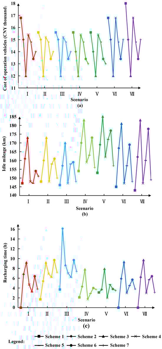
Figure 11.
Sensitivity analysis for the 3 objective function values in the 7 Scenarios. (a) Sensitivity analysis for the cost of operation vehicles (b) Sensitivity analysis for the idle mileage (c) Sensitivity analysis for the recharging time.
6. Conclusions
This study focuses on the multi-type EVS optimization problem. The objective is to achieve cost reduction for enterprises yielding to the deployment of vehicles, trip connection time, driving range, load capacity, and charging time. Unlike traditional vehicle scheduling methods, this paper focuses on multi-type vehicle scheduling, which attains energy optimization and environmentally friendly vehicle type compositions. Compared with single large-type vehicle schemes, the operation cost of multi-type vehicle scheduling on one-trip, two-trip, and three-trip frequency scenarios is reduced by 20.8%, 6.3%, and 9.1%, respectively.
A preprocessing-based GA is used to solve the model. As a result, we derive an optimized multi-type EVS scheme. The comparative analysis of the operation costs, idle mileage costs, and recharging time costs verifies the superiority of multi-type vehicle scheduling over single-type vehicle scheduling in different frequency scenarios. Compared with the single large-type scheme, the three-type vehicle scheme reduces the total cost by 20.7%, 6.2%, and 9.1%, respectively, in one-trip, two-trip, and three-trip frequency scenarios. Thus, multi-type optimization significantly reduces the total cost of electric PT.
Furthermore, a sensitivity analysis is conducted to evaluate vehicle scheduling schemes based on various weights/preferences. It is beneficial for obtaining quantifiable managerial insights on the impact of different cost alterations or unique emphasis. When balancing the vehicle operation cost, idle mileage, and recharging time, that is, if we consider them equally important, the total cost is reduced by about 17.08%. If we focus on reducing the vehicle operation cost and idle mileage, the total cost is about 11.78% lower than the maximum cost. If we focus on reducing the vehicle operation cost and recharging time, the total cost is reduced by about 17.08%, at most. If we focus on reducing the idle mileage and recharging time, the total cost is reduced by about 25.79%, at most.
In this paper, we model on the basis of a single depot scenario, which is beneficial for executing the trip tasks in strict accordance with the schedule. However, we do not allow for random travel times due to unexpected situations. The genetic algorithm can acquire an optimized solution quickly, however, algorithm enhancement is anticipated in the research plan. Future study plans can include the following:
- Expanding the optimization problem to multiple depots and addressing the network-level synchronization of scheduling problems.
- Considering the influence of emergencies, traffic congestion, and other special conditions on vehicle scheduling. Techniques such as GIS technology can be employed to study dynamic traffic network planning for pure electric vehicles.
- Simultaneously considering various charger types to optimize the charging infrastructure and scheduling process.
- Exploring the collaborative optimization of vehicle scheduling with crew scheduling to enhance the overall operational efficiency and cost-effectiveness.
Author Contributions
Conceptualization, Z.M., Z.C., Y.W. and S.Z.; methodology, Z.M., Z.C., Y.W. and S.Z.; software, Z.M., Z.C., Y.W. and S.Z.; validation, Z.M., Z.C., Y.W. and S.Z.; formal analysis, Z.M. and Z.C.; investigation, Z.M.; resources, Z.M.; data curation, Z.M.; writing—original draft preparation, Z.M., Z.C., Y.W. and S.Z.; writing—review and editing, Z.M., Z.C., Y.W. and S.Z.; visualization, Z.C.; supervision, Z.C. and S.Z.; project administration, Z.M., Z.C., Y.W. and S.Z.; funding acquisition, Z.M., Z.C., Y.W. and S.Z. All authors have read and agreed to the published version of the manuscript.
Funding
This study was supported by the National Natural Science Foundation of China (72101127) and (72101126), by The Science and Technology Planning Project of Suzhou City (No. SZS2022015), by CCF-Tencent Open Fund (CCF-Tencent IAGR20220111), by Guangdong Science and Technology Strategic Innovation Fund (the Guangdong–Hong Kong-Macau Joint Laboratory Program (2020B1212030009)), and by the Postgraduate Research & Practice Innovation Program of Jiangsu Province (SJCX23_1785).
Data Availability Statement
Data are contained within the article.
Conflicts of Interest
The authors declare no conflict of interest.
References
- Gavish, B.; Shlifer, E. An approach for solving a class of transportation scheduling problems. Eur. J. Oper. Res. 1979, 3, 122–134. [Google Scholar] [CrossRef]
- Wang, Y.; Liao, Z.; Tang, T.; Ning, B. Train scheduling and circulation planning in urban rail transit lines. Control Eng. Pract. 2017, 61, 112–123. [Google Scholar] [CrossRef]
- Mancini, S.; Gansterer, M. Vehicle scheduling for rental-with-driver services. Transp. Res. Part E Logist. Transp. Rev. 2021, 156, 102530. [Google Scholar] [CrossRef]
- Olariu, F.E.; Frasinaru, C. Multiple-Depot Vehicle Scheduling Problem Heuristics. arXiv 2020, arXiv:2004.14951. [Google Scholar] [CrossRef]
- Wu, M.; Yu, C.; Ma, W.; An, K.; Zhong, Z. Joint optimization of timetabling, vehicle scheduling, and ride-matching in a flexible multi-type shuttle bus system. Transp. Res. Part C Emerg. Technol. 2022, 139, 103657. [Google Scholar] [CrossRef]
- Jin, L. Study on the Matching Relationship between Electric Bus Battery State and Operation. Master’s Thesis, Beijing Jiaotong University, Beijing, China, 2011. (In Chinese). [Google Scholar]
- Sebastiani, M.T.; Lüders, R.; Fonseca, K.V.O. Evaluating Electric Bus Operation for a Real-World BRT Public Transportation Using Simulation Optimization. IEEE Trans. Intell. Transp. Syst. 2016, 17, 2777–2786. [Google Scholar] [CrossRef]
- Wang, Y.; Huang, Y.; Xu, J.; Barclay, N. Optimal recharging scheduling for urban electric buses: A case study in Davis. Transp. Res. Part E Logist. Transp. Rev. 2017, 100, 115–132. [Google Scholar] [CrossRef]
- Rogge, M.; Van der Hurk, E.; Larsen, A.; Sawer, D.U. Electric bus fleet size and mix problem with optimization of recharging infrastructure. Appl. Energy 2018, 211, 282–295. [Google Scholar] [CrossRef]
- Tang, X.; Lin, X.; He, F. Robust scheduling strategies of electric buses under stochastic traffic conditions. Transp. Res. Part C Emerg. Technol. 2019, 105, 163–182. [Google Scholar] [CrossRef]
- He, Y.; Liu, Z.; Song, Z. Optimal recharging scheduling and management for a fast-recharging battery electric bus system. Transp. Res. Part E Logist. Transp. Rev. 2020, 142, 102056. [Google Scholar]
- Yao, E.; Liu, T.; Lu, T.; Yang, Y. Optimization of electric vehicle scheduling with multiple vehicle types in public transport. Sustain. Cities Soc. 2020, 52, 101862. [Google Scholar] [CrossRef]
- Wang, J.; Kang, L.; Liu, Y. Optimal scheduling for electric bus fleets based on dynamic programming approach by considering battery capacity fade. Renew. Sustain. Energy Rev. 2020, 130, 109978. [Google Scholar] [CrossRef]
- Wu, W.; Lin, Y.; Liu, R.; Jin, W. The multi-depot electric vehicle scheduling problem with power grid characteristics. Transp. Res. Part B Methodol. 2022, 155, 322–347. [Google Scholar] [CrossRef]
- Liu, T.; Ceder, A.A. Battery-electric transit vehicle scheduling with optimal number of stationary chargers. Transp. Res. Part C Emerg. Technol. 2020, 114, 118–139. [Google Scholar] [CrossRef]
- Uslu, T.; Kaya, O. Location and capacity decisions for electric bus recharging stations considering waiting times. Transp. Res. Part D Transp. Environ. 2021, 90, 102645. [Google Scholar] [CrossRef]
- He, J.; Yang, H.; Tang, T.Q.; Huang, H.J. An optimal recharging station location model with the consideration of electric vehicle’s driving range. Transp. Res. Part C Emerg. Technol. 2018, 86, 641–654. [Google Scholar] [CrossRef]
- Ma, T.Y.; Xie, S. Optimal fast recharging station locations for electric ridesharing with vehicle-recharging station assignment. Transp. Res. Part D Transp. Environ. 2021, 90, 102682. [Google Scholar] [CrossRef]
- Xue, H. Multi-Vehicle Pure Electric Bus Timetable and Vehicle Scheduling Integration and Optimization. Master’s Thesis, Dalian Maritime University, Dalian, China, 2022. (In Chinese). [Google Scholar]
- Katoch, S.; Chauhan, S.S.; Kumar, V. A review on genetic algorithm: Past, present, and future. Multimed. Tools Appl. 2020, 80, 8091–8126. [Google Scholar] [CrossRef] [PubMed]


Disclaimer/Publisher’s Note: The statements, opinions and data contained in all publications are solely those of the individual author(s) and contributor(s) and not of MDPI and/or the editor(s). MDPI and/or the editor(s) disclaim responsibility for any injury to people or property resulting from any ideas, methods, instructions or products referred to in the content. |
© 2023 by the authors. Licensee MDPI, Basel, Switzerland. This article is an open access article distributed under the terms and conditions of the Creative Commons Attribution (CC BY) license (https://creativecommons.org/licenses/by/4.0/).